Characterization and validation of thermal and boron mixing phenomena in the downcomer and lower plenum of an integrated primary system nuclear reactor

(1)

(2)

Consorzio Interuniversitario per la Ricerca TEcnologica Nucleare

Lavoro svolto in esecuzione dell’Attività LP2-D2

AdP MSE-ENEA sulla Ricerca di Sistema Elettrico - Piano Annuale di Realizzazione 2011 Progetto 1.3.1 “Nuovo Nucleare da Fissione:

collaborazioni internazionali e sviluppo competenze in materia nucleare”

UNIVERSITA’ DI PISA

Dipartimento di Ingegneria Meccanica, Nucleare e della Produzione

Characterization and validation

of thermal and boron mixing phenomena

in the downcomer and lower plenum

of an integrated primary system nuclear reactor

(Caratterizzazione e qualifica della fenomenologia

del miscelamento termico e del boro

nel lower plenum e nel downcomer

di un reattore PWR di tipo integrato)

Authors:

Ignazio Angelo

Vincenzo Baudanza

Nicola Forgione

Daniele Martelli

CERSE‐UNIPI RL 1522/2011

Pisa, August 2012

2

(3)

2

Index

Summary ... 3

1. Introduction ... 4

2. Facility description ... 5

2.1 Test section...5

2.2 Hydraulic circuit...7

2.3 Instrumentation...8

2.4 Data acquisition system...10

3. Numerical simulation ... 11

3.1 RELAP5 analysis...11

3.1.1 Circuit nodalization... 11 3.1.2 Simulation test matrix and obtained results ... 12

3.2 CFD simulations ...14

3.2.1 Computational domain... 14 3.2.2 Numerical model ... 15 3.2.3 Obtained results ... 15

4. Experimental tests ... 20

4.1 Test matrix ...20

4.2 Test procedure...20

4.3 Obtained results ...21

5. Conclusions ... 27

References ... 28

Nomenclature ... 28

Breve CV del gruppo di lavoro...29

(4)

3

Summary

The main objective of this work is to present the preliminary results obtained in the recent experimental campaign performed at the DIMNP (Dipartimento di Ingegneria Meccanica, Nucleare e della Produzione) of the University of Pisa with a stainless steel mock‐up, simulating the downcomer and lower plenum of a small scale PWR (Pressurized Water Reactor). In particular, the facility, characterized by a scaling factor of 1/5 in respect to a reference reactor having steam generators integrated inside the vessel, was designed in order to provide relevant data to study the mixing phenomena occurring during a DVI (Direct Vessel Injection) line break accident, SB‐LOCA (Small Break Loss Of Coolant Accident), and to validate commercial CFD (Computational Fluid Dynamic) codes.

In the first part of the report a detailed description of the experimental facility is provided including the hydraulic circuit and the data acquisition system. In this context, the correct test procedure has been supported and validated by numerical simulations performed using the RELAP5 code.

The second part of the work is mainly focused on numerical simulations, performed using the Fluent CFD code, of the mixing phenomena occurring during water injection into the vessel from the two lines representing the two DVIs.

The final and most important part of the report was devoted to the description of the first performed experimental activity and to the critical analysis of the obtained test results. The six experimental tests analysed in this part give useful information concerning thermal mixing in the lower plenum of the facility test section.

(5)

4

1. Introduction

The mixing phenomena of the coolant in a nuclear reactor is an important mechanism of intrinsic safety against dilution of boron. In a PWR, the boric acid is added to the coolant in such a way as to compensate the excess reactivity of the fuel [1]. The long term reactivity control, in normal operating conditions, is obtained with variation of the concentration of boron, dissolved in the form of boric acid in the water of the primary loop. Non‐uniformity in the mixing of boron is one of the most important safety topics of light water reactors; in fact, under certain operating or incidental conditions, it is possible to have the formation of a fluid plume at low boron concentration in the primary loop that, entering the core, without being mixed with water at the nominal boron concentration, may induce the risk of an accident for insertion of positive reactivity [2].

The mixing phenomena is not only important for nuclear safety, but also for structural integrity. In the case of LOCA, the cold water of the ECCS (Emergency Cooling System) is injected into the primary hot loop. When the cold water comes into contact with the vessel walls, thermal stresses occur, which can compromise reactor pressure vessel integrity [3]. The mixing phenomena is also important during normal operation of the reactor, for example relating to the distribution of the coolant temperature at the inlet of the core in the case of partial shutdown of the primary coolant pumps. There are currently two methods for studying the boron mixing in the downcomer of a PWR: • Experiments on a reactor scale model: the approaches of dynamic similarity ("scaling") for the flows in forced convection permit the use of a relatively small scale model (e.g., 1/5), while for the natural convection flows larger and more expensive equipment to apply the "scaling" are necessary [4]; • Numerical simulation: the rapid development of computers has made the use of CFD techniques for the study of problems involving elements with three‐dimensional geometries of large sizes possible [4]. However, in nuclear applications, numerical models require an initial experimental campaign in order to validate the results obtained by code simulations with results obtained experimentally. For this reason the most common procedure to study boron mixing in a downcomer and lower plenum of a PWR is a combined experimental and numerical approach [4]. This work was performed in the frame of the research programme on “New Nuclear Fission” funded by our Ministero dello Sviluppo Economico (Ministry of Economical Development) and co‐ordinated by ENEA. In particular, it is oriented to perform a preliminary experimental campaign on a mock‐up simulating the downcomer and lower plenum of a small scale pressurized reactor, categorized as Integrated Primary System nuclear Reactor (IPSR), in order to provide relevant data to study the mixing phenomena occurring during a DVI line break accident and to validate commercial CFD codes.

In the present report, after a description of the experimental facility, the results of pre‐test simulations carried out with the RELAP5 system code [5] and Fluent [6] CFD code are presented. In particular, the pre‐test calculations by the RELAP5 code should provide useful indications for the maximum pressure acting inside the test section during normal and filling operations, necessary for the mock‐up design. Instead the Fluent pre‐test simulations were conducted in order to identify relevant phenomena in the downcomer and lower plenum, like vortex formation, recirculating regions and mixing characteristics, thus setting up the appropriate instrumentation and locating them in more significant positions.

In the last part of the report the experimental results obtained in the first experimental campaign, recently performed at DIMNP of the Pisa University, are presented and discussed.

(6)

5

2. Facility description

2.1 Test section

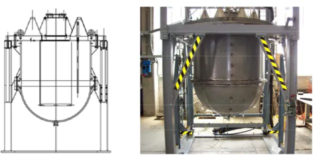
The experimental facility, built at the DIMNP of Pisa University, consists of a 1:5 scaled model of downcomer and lower plenum of the IRIS (International Reactor Innovative and Secure) reactor [7], designed with particular care to represent the geometrical configuration of the real plant (see red zone marked in Figure 2.1).

In Figure 2.2 the test section is shown as drawing and as a photo performed on the lateral side. The geometrical similarity between the test section and the original reactor is respected until the core inlet, which is not reproduced in the facility and which is then excluded from the similarity. The test section is composed of a lower semi‐spherical shell of stainless steel having a radius of 0.629 m and a thickness of 6 mm that represents the lower plenum, connected to a cylindrical wall having the same radius of the shell and a length of 0.818 m. An internal stainless steel cylinder having an external radius of 0.285 m and longer in respect to the external cylinder, completes the downcomer region. In the upper part of the facility, eight conical stainless steel pipes simulate the eight downcomer mass flow inlets coming from the eight IRIS steam generators (not reproduced in the facility). Two stainless steel tubes, representing the two DVI lines of the IRIS reactor, are also considered with a nominal length of 0.804 m and an internal diameter of 0.0158 m. Figure 2.1: IRIS reactor with the marked downcomer and lower plenum region.

(7)

6 Figure 2.2: Test section: drawing (left) and photos (right). Due to the particular geometry of the conical pipes, in order to avoid the problem of detachment of the boundary layer, flow dividers were added inside them making the water velocity entering in the downcomer region uniform (see Figure 2.3). Figure 2.3: Construction detail of the divider flow. A perforated plate was installed at the inlet section of the inner cylinder, avoiding non‐uniform velocity at the entrance observed during preliminary numerical simulations. The plate’s hole arrangement is similar to that provided for the core inlet section in the reference plant [6] (see Figure 2.4).

(8)

7

2.2 Hydraulic circuit

The facility layout shown in Figure 2.5, consists of 3 different pipe lines:

‐ the primary line, in which warm water, at a maximum temperature of 50°C, is sent to a manifold where the flow rate is equally divided among eight conical stainless steel pipes, simulating the eight downcomer mass flow inlets coming from the IRIS steam generators; ‐ the secondary line, which provides the required cold water flow to the two pipes simulating the DVIs located inside the IRIS downcomer; ‐ the tertiary line, which controls the warm fluid temperature (water from the primary line). Figure 2.5: Layout of the facility. The warm water, passing through the primary line, comes from a large water reservoir. The temperature of about ten cubic meters of water, contained in this large reservoir, was controlled by a heater system which includes three electrical heaters with a total maximum electrical power installed of 9 kW. Before starting the experimental test, the water contained in the large reservoir was heated at the desired temperature (less or equal to 50°C) circulating it in the tertiary loop only (acting on a three way valve). After the temperature set point was reached, the warm water was circulated through the primary line into the manifold and the heater system was bypassed. The high thermal capacity of the stored reservoir water allows tests to be performed in about one hour, without the activation of the HS, with a negligible reduction in water temperature inside the test section. When a test using cold water injection was foreseen the secondary line was also activated, injecting cold water from one or both the DVI pipes. In each pipe a needle valve is present to precisely regulate the flow rate of the fluid. The flow rate in each of the two DVI pipes was measured through a differential pressure sensor connected to the Venturi device incorporated in the body of the valve.

(9)

8

2.3 Instrumentation

The measuring instrumentation available up to now includes: • K‐type TCs (thermocouples), to monitor the inlet and outlet test section fluid temperatures and fluid temperatures at different locations inside the test section, to monitor temperature variations mainly in the lower plenum and at the “core inlet section”;

• an electromagnetic flow meter, placed on the pipe coming from the reservoir and shared with the primary and tertiary line;

• two differential pressure sensors used to evaluate and to control the flow in the two DVI pipes. All the measuring instruments have been calibrated by the manufacturer (as the electromagnetic flow meter) or directly in the laboratory (as for the TCs), to assess the uncertainty affecting every experimental data.

During the shake‐down tests problems were encountered on the data repeatability related to the evaluation of the mass flow rate injected from the two DVI lines. These data are obtained as an indirect evaluation through the measure of differential pressure on a Ventury type nozzle present in each of the two DVI pipes. To overcome this problem, allowing a fast execution of a preliminary matrix of test, we decided to perform, in this phase, tests with cold water injection from only one of the two DVI pipes and with a fixed injection flow rate of 0.1 kg/s. Then, a special flow rate regulator, able to maintain a quite constant flow rate for a wide range of operating pressure difference conditions, was placed in one of the two DVI pipes.

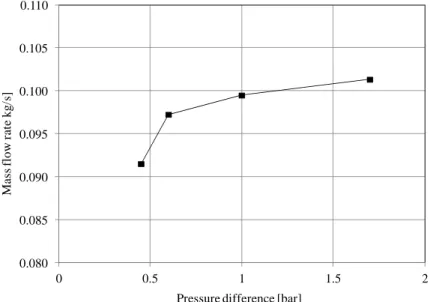
To verify the behaviour of this regulator, before the execution of experimental tests, a check of its calibration was performed considering four different working conditions in correspondence of four different pressure differences. These tests consisted in flowing water through the regulator valve inserted in the DVI line and collecting the water for a certain period of time. After weighting the water collected with more precise scales it was possible to calculate the associated water mass flow rate. The obtained trend of the flow rate as a function of the pressure difference value is reported in Figure 2.6. As can be seen the water flow rate is not perfectly constant, but if the pressure difference through the regulator is maintained between 0.8 and 1.5 bar the obtained mass flow rate is equal 0.1 kg/s with a maximum deviation of about 1%. In performing the experimental tests the pressure difference through this regulator was set to about 1.2 bar. 0.080 0.085 0.090 0.095 0.100 0.105 0.110 0 0.5 1 1.5 2 Mass f low r at e k g /s]

Pressure difference [bar]

(10)

9

In Figures 2.7 and 2.8, respectively, the final disposal of the TCs that are placed just above the perforated plate and of those placed inside the semi‐spherical shell in correspondence to the horizontal plane placed 7 cm below the inlet section of the inner cylinder are shown.

In the semi‐spherical region there are other three TCs (H3, I3 and L3) that are inserted for

4 cm inside the inner surface of the metallic shell, at an elevation of 12 cm above the inlet section of the inner cylinder (see Figure 2.9). The positions of two of these three TCs are shown in Figure 2.9. The third TC (L3) remains on the same horizontal plane as the other two, but on the plane

perpendicular to that shown in Figure 2.9, on the same side where the TCs L1 and L2 are placed.

Figure 2.7: Disposal of the TCs placed above the perforated plate. Figure 2.8: TCs inside the semi‐spherical part of the test section placed on the horizontal plane at 7 cm below the inlet section of the inner cylinder.

(11)

10

Figure 2.9: TCs placed in the symmetry vertical plane containing the axes of the two DVIs.

2.4 Data acquisition system

The DAS (Data Acquisition System), utilized for the facility, converts and acquires the electrical signals coming from instrumentation present in the facility. In particular, the sensors are TCs, differential pressure transducers and flow meters. The DAS is a network data logger based on National Instruments® devices and software. It mainly consists of:

• one external SCXI (Signal Conditioning eXtensions for Instrumentation) 1001, 12‐Slot chassis that is used for lodging data conditioning modules to be multiplexed on the DAQ (Data Acquisition) board and the DAQ itself;

• one DAQ and control module SCXI‐1600 of USB type on board at the chassis SCXI 1001;

• two modules of SCXI‐1102B with 32 channels each (additionally equipped with a SCXI‐1303 front mounting terminal block) for acquiring signals up to 32 TCs each or other signals of tension;

• two SCXI‐1125 8‐channel programmable isolated input modules equipped with a SCXI‐1327 front mounting terminal block for acquiring general signals of voltage with galvanic isolations.

To drive the DAQ boards and the signal conditioning modules the program LabVIEW® (Laboratory Virtual Instrument Engineering Workbench) was used. The acquisition program was set up by using “virtual instruments” available in the package.

(12)

11

3. Numerical simulation

3.1 RELAP5 analysis

3.1.1 Circuit nodalization A pre‐test analysis of the hydraulic circuit, was performed (using the RELAP5 system code [5]) in order to verify that the pressure inside the test section does not exceed the design value of 0.5 barg. The RELAP5 nodalization, developed to simulate all the three lines of the hydraulic circuit, is shown in Figure 3.1. In the input used for the analysis, each component is divided into sub volumes (hydrodynamic cells) whose number is equal to the ratio between the length of the component and the "unitary" length of a sub volume that has been taken, for this calculation, equal to about 5 cm. The circle present at some junctions indicates the presence of a concentrated pressure drop due to the change of direction of the pipe.

The entire circuit can be schematically divided into three main sections:

‐ Delivery: starting from Tmdpvol‐1 (z = 0) to the Pipe‐250. At the first component (Tmdpvol‐1) pressure is fixed at 1.3 bar and temperature is fixed at 50°C, and represents the tank located upstream of the circuit. Downstream the reservoir is placed the primary pump (Tmdpjun‐2) which provides the desired flow inside the pipes. The water flows in the delivery circuit, through the piping shown schematically, going from Pipe‐170 to Pipe‐180 up to the collector, Branch‐210 (z = 3.33 m), which divides into eight uniform flow the total amount of fluid.

‐ Test Section: it is composed of Annulus‐260 (z = 1.91 m), which represents the outer cylindrical part of the test section and a lower hemispherical part of the shell, until the level at which the input section of the inner cylinder arrives. This component has been divided into sub‐volumes of different sections in order to reproduce the variation of the cross‐sectional area. Connected to that component, there is Branch‐270 (z = 0.77), which represents the hemispherical bottom part not incorporated in the Annulus‐260. This component has two inputs, one for the inlet of water from the cones and the other for the inlet of water from the two DVI tubes and one outlet through which the fluid rises along the inner cylinder (Pipe‐280) and exits through the nozzle outlet, the Pipe‐290 (z = 2.11 m). The circuit of DVI, connected to Branch 270, is realized with the components between Tmdpvol‐885 (where pressure is fixed at 1.3 bar and temperature at 50°C) and Pipe‐901. The pump is represented by the Tmdpjun‐886, which imposes a certain flow rate depending on the considered test. ‐ Return: starts from Pipe‐300 (z = 2.29 m start level pipe), in which the fluid goes back upwards until Pipe 310 (z = 2.49 m), descending then up to a height z = 0 (fromPipe‐317 until Pipe‐360) and finally arrives at the exit in which the fluid flows into the initial tank, schematized by Tmdpvol‐450 (z = 3.53 m), in which pressure is fixed at 1 bar and temperature at 20°C.

(13)

12 Pipe 10 J-15 Pipe 20 Pipe 30 Pipe 40 Pipe 50 J-45 J-55 Pipe 60 Pipe 70 J-65 J-75 Pipe 80 J-85 Pipe 90 J-95 Pipe 100 J-105 Pipe 110 J-115 Pipe 120 J-125 Pipe 130 J-135 Pipe 140 J-145 Pipe 150 Pipe 160 J-165 Pipe 170 J-177 Pipe 180 Pipe 190 Pipe 200 Branch 210 J-215 Pipe 220 _J-225 Pipe 240 J-235 Pipe 230 J-245 Pipe 250 J-255 Anulus 260 Anulus 260 Branch 270 Pipe 280 Pipe 290 Branch-295 Pipe 300 Pipe 310 J-305 J-315 Pipe 325 J-326 Pipe 330 Pipe 340 J-345 Pipe 350 Pipe 360 J-365 Pipe 370 J-375 Pipe 380 J-395 J-405 … … … … … … … x8 J-285 Pipe 390 Pipe 400 J-415 Pipe 410 J-425 Pipe 420 J-435 Tmdpvol 450 P= 1 bar T= 20 °C Pipe 430 Pipe 440 J-445 Tmdpvol 1 P= 1.3 bar T= 50 °C Tmdpjun 2 Tmdpvol 885 P= 1.3 bar T= 20 °C Tmdpjun 886 Pipe 901 Pipe 910 J-915 Pipe 920 Tmdpvol 930 P= 1 bar T= 20 °C Pipe 317 _Pipe 176 Valvola 171 Branch-173 Valvola 945 Branch-322 Tmdpvol 208 P= 1 bar T= 20 °C Branch 205 Pipe 206 Valvola 175 Valvola 318 Valvola 325 Valvola 207 Tmdpnvol 882 P=1 bar T=293.15 K Branch 894 Pipe 884 Valvola 883 Pipe 898 Pipe 892 Pipe 889 Pipe 887 J-888 J-890 Z = 8.17 Z = 1.91 Z = 0.77 Z = 0 Z = 0 Z = 5.27 Z = 3.53 Z = 5.33 Z = 3.33 Z = 2.49 Z = 3.27 Figure 3.1: RELAP5 Nodalization. 3.1.2 Simulation test matrix and obtained results The test matrix of the performed simulations is reported in Table 3.1. Table 3.1: RELAP5 simulation test matrix. Test Primary Pump (Tmdpjun‐2) [kg/s] DVI Pump (Tmdpjun‐886) [kg/s] Test I 1.5 0.1 Test II 1.5 0.05 Test III 1 0.1 Test IV 1 0.05

In the present analysis, the two valves relative to the two outlets (Valve 207 and Valve 883) and the additional valve for the reversal flow (Valve 945) are closed. The simulations were carried out considering the circuit being initially filled with water. The activation of the pumps is delayed by 200 s in such a way that the RELAP5 code statically balances the water level present inside the piping, particularly the amount of liquid inside the vent pipes. At time t = 200 s, the primary pump is activated (Tmpdpjun‐2) gradually opening to the desired flow rate value after 10 s (ramp 10 s). At time t = 230 s the DVI pump is activated (Tmdpjun‐886) imposing a gradual opening with a ramp of 5 s. The

(14)

13 gradual activation of the pump is necessary in order to avoid pressure oscillations that may damage the hydraulic circuit. The obtained results are reported in terms of: ‐ transient pressure trend on the upper test section region; ‐ water mass flow rate from the pumps; ‐ pressure value along the hydraulic circuit in steady state conditions. The results of the comparison between Test I and Test III are shown from Figure 3.2 to Figure 3.4 (see Table 3.1). 0.0 0.2 0.4 0.6 0.8 1.0 1.2 1.4 1.6 1.8 0 50 100 150 200 250 300 350 400 450 500 M as s fl ow ra te [ kg/ s] Time [s] Test I Test III Figure 3.2: Water mass flow rate from the pumps.

From this comparison it has been noted how pressure values in Test I are larger than Test III, but in particular are higher than those considered in the design phase for the test section. In conclusion the tests that can be realized in the first experimental campaign are Test III and Test IV, with a maximum mass flow rate value of about 1 kg/s. 1.0E+05 1.1E+05 1.2E+05 1.3E+05 1.4E+05 1.5E+05 1.6E+05 1.7E+05 1.8E+05 0 50 100 150 200 250 300 350 400 450 500 P re ss u re [P a] Time [s] Test I Test III Figure 3.3: Transient pressure trend versus time simulation on the upper test section region.

(15)

14 1.00E+05 1.20E+05 1.40E+05 1.60E+05 1.80E+05 2.00E+05 2.20E+05 2.40E+05 P ressu re [P a ]

Hydraulic circuit components

Test I (1.6 kg/s) Test III (1.1 kg/s) DELIVERY RETURN 1.36 bar 1.59 bar Figure 3.4: Pressure value along the hydraulic circuit in steady state conditions.

3.2 CFD simulations

The more detailed description of the computational domain and of the adopted numerical model was reported in a previous work [8]. Here a short description of the over mentioned items are presented to understand the new obtained results better. 3.2.1 Computational domain The adopted 3D geometrical domain of the test section is shown in Figure 3.5. It must be noted that, because of symmetry, only half a test section was reproduced. As can be seen from Figure 3.5, the origin of the coordinate reference system is positioned just on the symmetry plane at the vertical level in which the cylindrical part is connected to the spherical bottom part. The domain was discretized using an unstructured mesh of different sizes in order to reduce the dimension of the grids in those areas that are of most interest from a fluid‐dynamic point of view (see Figure 3.6). The total number of cells needed for the domain is about 4,700,000 with smaller cell sizes in the region of DVI pipe and near the cross section representing the core inlet. Figure 3.5: Geometrical domain and reference system.

(16)

15 Figure 3.6: Spatial discretization: symmetry plane(left) and enlarged view of the mesh near the DVI's pipe(right). 3.2.2 Numerical model Since the Reynolds number assumes relatively high values in the downcomer, turbulent mixing is more important than molecular diffusion. Therefore, temperature and boron concentration profiles become similar once both the turbulent diffusivity coefficients assume values of the same order of magnitude. Based on this assumption, in the facility the temperature field related to the mixing processes in the downcomer and lower plenum was investigated instead of boron concentration distribution.

The working fluid considered in the simulations is water with the density set in the code as a function of temperature.

In the performed simulations, regarding the perforated plates placed into the eight conical pipes and in the inner cylinder, two different models have been used. In the first case, each perforated plate is simulated as a porous region by the porous media model option [5]. This model consists of adding a source term in the equations of the standard flow which is composed of two parts: a viscous loss term and an inertial loss term. In the case of the perforated plate, it is possible to neglect the viscous loss term and consider only the inertial loss.

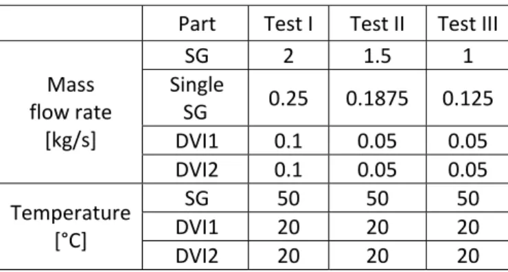
Instead, the porous jump model [5] has been used in simulating the perforated plate placed into the inner cylinder. 3.2.3 Obtained results From simulations carried out in previous studies [9‐10], performed using the RELAP5 system code, the water mass flow rate conditions for the inlet section in the downcomer and DVI of the real reactor were obtained as a result of accidental scenario analysis (breaking of one of the two DVIs). Since it was not possible to reproduce experimental test conditions with relatively high water flow rates due to the high pressure involved, a criterion of scaling has been adopted. This criterion is based upon the concept in conserving the residence time of the fluid inside the downcomer. Values of water temperature in the test section were assumed respectively equal to 50°C for the water entering the downcomer through the eight conical pipes and 20°C for the water entering from the DVI. As a result of these considerations, the simulation test matrix, shown in Table 3.2, has been considered.

(17)

16

Table 3.2: CFD simulation test matrix.

Part Test I Test II Test III

SG 2 1.5 1 Single SG 0.25 0.1875 0.125 DVI1 0.1 0.05 0.05 Mass flow rate [kg/s] DVI2 0.1 0.05 0.05 SG 50 50 50 DVI1 20 20 20 Temperature [°C] DVI2 20 20 20

For each test, steady state condition has been initially simulated without activation of the two DVI tubes. This preliminary simulation is required in order to define a correct initial condition from which a transient analysis is performed for the study of the flow and temperature field following the activation of the cold water injection from the two DVIs. Considering the duration of the experimental tests and the computational time required for the test simulation, the first 200 s of transient has been simulated. In fact, the main changes in temperature at the inlet core surface occurs during the first 100 s, after which there are slow changes in the average temperature (less than 0.5°C every 100 s).

The obtained results are shown only for Test I because the same observations and conclusions can be made for Tests II and III.

The results are analyzed in terms of temperature and velocity fields. The used units are [°C] for the temperature and [m/s] for the velocity. The simulation results are shown on two main planes: the symmetry plane and the ones normal to it. In Figure 3.7 temperature distribution on the plane normal to the symmetry plane is shown for Test I at t = 40 s of transient. Figure 3.7: Temperature distribution on the plane normal to the symmetry plane, for Test I (t = 40 s). As can be seen from Figure 3.7, there is a marked stratification between the two fluids, highlighted by the different colours of the hot fluid (red) and the mixed fluid at the bottom hemispherical region. This stratification is due to the different densities between the two water flows and to the higher velocity of the cold flow that exits the DVI tubes, combined with the geometry of the test section.

(18)

17 Figure 3.8 shows the temperature distribution on the symmetry plane for the same test and at the same instant as Figure 3.7. Figure 3.8: Temperature distribution on the symmetry plane for Test I (t = 40 s). A "U" shape distribution of the temperature at the entrance of the core can be noted. This effect is due to the fact that fluid velocity at the inlet of inner cylinder does not have a negligible radial component and hence the fluid tends to move and pass next to the external side of the perforated plate. Such distribution of fluid velocity is shown in Figure 3.9, where the velocity distribution on the symmetry plane is reported for t = 40 s. Figure 3.9: Velocity distribution on symmetry plane for Test I (t = 40 s). The analysis of Figure 3.9 put in evidence the formation of vortices in the lower part of the downcomer, mainly due to the water jet from the two DVIs, that tend to radially drive the fluid to the entrance of the

(19)

18

core region. This radial component of velocity is reduced inside the cylinder by the walls straightening the fluid after a central stagnating zone at the exit of the perforated plate.

Pre‐test analysis can give useful information about the arrangement of the measuring probes (such as TCs) in the experimental campaign. From the performed analysis it was observed that the regions where temperature gradients mainly occur are at the core entrance and the region between the exits of the DVI and the inner wall of the vessel. These two patterns are shown, respectively, in Figures 3.10 and 3.11. 46.5 47.0 47.5 48.0 48.5 49.0 49.5 50.0 50.5 -0.6 -0.4 -0.2 0.0 0.2 0.4 0.6 0.8 1.0 1.2 T emp er at u re [ °C] z coordinate [m] t = 40 s t = 100 s t = 200 s Figure 3.10: Temperature distribution along the DVI axis between the exits of the DVI and the inner wall of the vessel for the Test I. 46.5 47.0 47.5 48.0 48.5 49.0 49.5 50.0 50.5 -0.30 -0.25 -0.20 -0.15 -0.10 -0.05 0.00 0.05 0.10 0.15 0.20 0.25 0.30 T e m p er at u re [ °C] y coordinate [m] t = 40 s t = 100 s t = 200 s Figure 3.11: Temperature distribution on the core inlet section for the Test I.

In Figure 3.12 is instead reported the average temperature on the inlet section of the inner cylinder, where the perforated plate is placed. It can be seen a fast temperature decrease of about 1.5°C in the first seconds of the transient, followed by a more gradual reduction in the temperature trend.

(20)

19 46 47 48 49 50 51 52 0 20 40 60 80 100 120 140 160 180 200 T em p er at u re [ °C ] Time [s] Figure 3.12: Average temperature time trend on the core inlet section for the Test I.

(21)

20

4. Experimental tests

4.1 Test matrix

Six different tests were performed with three different values of the nominal mass flow rate of the warm water injected through the SGs (see Table 4.1). In particular, the first two tests (Test 1 and Test 2) are related to a nominal value of the mass flow rate of 1 kg/s and temperature of the injected warm water of 40 and 44°C, respectively. The next two tests (Test 3 and Test 4) are characterized by a nominal value of the mass flow rate of 0.75 kg/s and a temperature of the injected warm water of 42.5 and 42°C, respectively. The last two tests (Test 5 and Test 6) correspond to a nominal value of the mass flow rate that is half of that of the first two tests and with a temperature of 43.5 and 39.5°C, respectively. Table 4.1: Experimental test matrix.

Part Test 1 Test 2 Test 3 Test 4 Test 5 Test 6 SGs 1.029 1.035 0.768 0.767 0.524 0.576 DVI1 ‐ ‐ ‐ ‐ ‐ ‐ Mass flow rate [kg/s] DVI2 0.1 0.1 0.1 0.1 0.1 0.1 SGs 40 44 42.5 42 43.5 39.5 DVI1 ‐ ‐ ‐ ‐ ‐ ‐ Temperature [°C] DVI2 27.1 27.1 27.7 28.0 27.1 27.1

4.2 Test procedure

The test procedure consist in the initial start of the warm water injection from the eight conical entrances with the appropriate mass flow rate, waiting for the reaching of as uniform as possible water temperature inside the test section. Then, a first phase of some seconds of cold water injection from the DVI follows, having the purpose of cooling the pipeline that connects the cold water reservoir with the tests section. Due to the absence of thermal insulation on the external walls of the test section, thermal stratification phenomenon was observed inside the vessel, especially concentrated in the lower plenum. In fact, on the bottom side of the spherical region the temperature can result 2‐3°C lower than the water temperature inside the downcomer. To avoid this phenomena during circulation of the warm water, just before the start of the test, a certain quantity of water was initially discharged from the bottom side of the spherical region, opening the discharging valve and checking temperature distribution inside the test section by looking at the data acquisition system. When an almost uniform water temperature was obtained inside all the test section, i.e. with a temperature variation less than 0.5°C, the cold water injection was started through the DVI2, maintaining the DVI1 closed. In this first experimental campaign the duration of each test was set in the order of 12‐15 minutes.

(22)

21

4.3 Obtained results

In Figure 4.1 the time trend of both the temperatures of the TC placed at the exit section of the DVI inside the vessel (TC‐DVI2) and that positioned at the center of the perforated plate (TC‐F) is reported. In the same figure the mass flow rate of the warm water entering from the eight conical pipes is also reported. After looking at these time trends, we decided to fix the beginning of the thermal mixing test with the instant corresponding with the start of the fast reduction of the TC‐DVI2 temperature. As can be seen from Figure 4.1 the injection of cold water from the DVI2 line gives a reduction of about of 2°C on the center of the perforated plate. This reduction required about 100 s of transient from the beginning of the cold water injection to reach the asymptotic value and the temperature reduction starting with a delay of about 40 s in respect to what was observed for the TC‐DVI2.

The same temperature trend of the TC‐F can be observed for all the TCs placed above the perforated plate (see Figure 4.3). Looking with more attention at the trends reported in Figure 4.3, it is possible to note the TC‐A and the TC‐F undergoing a greater reduction in temperature respect to the other TCs placed at the same level. This means that the cold water injected from the DVI2 flows upward through the inner cylindrical shell preferentially on the opposite radial side respect to the injection position. This behaviour is confirmed by examination of the temperature measured from the TCs placed on the horizontal plane at 7 cm below the “core inlet” (see Figure 4.3). As it can be seen, the TC‐I1, placed on the opposite radial side respect to the DVI2, shows the lower temperature value respect to the other TCs. The temperature differences in the temperatures on the “core inlet section” are in this case in the order of a maximum of 0.5°C. A bigger temperature variation, of about 3°C, is observed for the TC‐F in the Test 5, characterized by a lower mass flow rate and a higher temperature of the warm water entering from the eight cones (see Figure 4.4). The temperature non uniformity at the “core inlet section” seems evident also in this test (see Figure 4.5). In this case the TC‐I1 shows a more significantly lower value of temperature respect to the other TCs placed on the same plane (see Figure 4.6). The operative conditions on which this test was executed required a long transient time respect to that considered for this experimental campaign. In fact, for Test 3 the 700‐900 s of monitored time interval is not sufficient to reach steady state conditions for temperature distribution inside the test section. In Figure 4.7 is possible to compare the TC‐I1 temperature measured from both tests 1 and 2 characterized by a nominal SGs mass flow rate of 1 kg/s. After a first fast temperature reduction of 2‐3°C, its value gradually increases, especially for Test 2. In tests 3 and 4, characterized by a nominal value of the SGs mass flow rate of 0.75 kg/s, instead the TC‐I1 shows, after the first rapid reduction, an almost uniform temperature trend (see Figure 4.8). For tests 5 and 6, characterized by a nominal value of the SGs mass flow rate of 0.5 kg/s, instead the TC‐I1 shows, after the first reduction, a gradual decrease in the temperature value (see Figure 4.9). This is coherent with the fact that for these last two tests the cold mass flow rate of the water injected from the DVI became on the same order of magnitude of the warm water mass flow rate. From the analysis of the previous results we can affirm that the next series of experimental tests must be performed with a longer recording time and, possibly, with temperature difference between the cold and warm water flows as greater as possible. The higher value of the warm water temperature is limited to the maximum design value of 50°C. For this reason the cold water coming from the DVI lines should be cooled before the injection in the test section to obtain a value in the order of 10°C. In this way the temperature difference between the warm and the cold water flows will be three times greater than the value obtained for the first series of experimental tests and the non‐uniformity of temperature distribution will be much more emphasized.

(23)

22 0 10 20 30 40 50 60 70 26 30 34 38 42 46 50 4100 4200 4300 4400 4500 4600 4700 4800 F lo w r a te [ l/min ] Te m p e ra tu re [ °C ] Time [s] TC-F TC-DVI2 Flow rate Start of the cold water injection from the DVI2 Figure 4.1: Temperature and mass flow rate time trends (Test 1). 34 36 38 40 42 44 46 4100 4200 4300 4400 4500 4600 4700 4800 T e m p er at u re [ °C ] Time [s] TC-A TC-B TC-C TC-E TC-F Start of the cold water injection from the DVI2 Figure 4.2: Temperature time trends from TCs placed above the perforated plate (Test 1).

(24)

23 34 36 38 40 42 44 46 4100 4200 4300 4400 4500 4600 4700 4800 T e m p er at u re [ °C ] Time [s] TC-G1 TC-G2 TC-H3 TC-I1 TC-I2 Start of the cold water injection from the DVI2 Figure 4.3: Temperature time trends from TCs located on the horizontal plane placed at 0.07 m below the inlet section of the inner cylinder (Test 1). 0 5 10 15 20 25 30 35 26 30 34 38 42 46 50 5700 5800 5900 6000 6100 6200 6300 6400 F lo w r a te [ l/min ] T e m p er at u re [ °C ] Time [s] TC-DVI2 TC-F Flow rate Start of the cold water injection from the DVI2 Figure 4.4: Temperature and mass flow rate time trends (Test 5).

(25)

24 34 36 38 40 42 44 46 5700 5800 5900 6000 6100 6200 6300 6400 T e m p er at u re [ °C ] Time [s] TC-A TC-B TC-C TC-E TC-F Start of the cold water injection from the DVI2 Figure 4.5: Temperature time trends from TCs placed above the perforated plate (Test 5). 34 36 38 40 42 44 46 5700 5800 5900 6000 6100 6200 6300 6400 T e m p er at u re [ °C ] Time [s] TC-G1 TC-G2 TC-H3 TC-I1 TC-I2 Start of the cold water injection from the DVI2 Figure 4.6: Temperature time trends from TCs located on the horizontal plane placed at 0.07 m below the inlet section of the inner cylinder (Test 5).

(26)

25 36 37 38 39 40 41 42 43 44 0 200 400 600 800 T e m p er at u re [ °C ] Time [s] Test 1 Test 2 Figure 4.7: Temperature time trends from TC‐I1 located on the horizontal plane placed at 0.07 m below the inlet section of the inner cylinder (Test 1 and Test 2). 36 37 38 39 40 41 42 43 44 0 200 400 600 800 T e m p er at u re [ °C ] Time [s] Test 3 Test 4 Figure 4.8: Temperature time trends from TC‐I1 located on the horizontal plane placed at 0.07 m below the inlet section of the inner cylinder (Test 3 and Test 4).

(27)

26 36 37 38 39 40 41 42 43 44 0 200 400 600 800 T e m p er at u re [ °C ] Time [s] Test 5 Test 6 Figure 4.9: Temperature time trends from TC‐I1 located on the horizontal plane placed at 0.07 m below the inlet section of the inner cylinder (Test 5 and Test 6).

(28)

27

5. Conclusions

The aim of this work is to present the experimental and numerical analysis of thermal mixing in a test section that reproduces the downcomer and the lower plenum of an integrated PWR reactor (IPSR) with a scaling factor of 1/5. The thermo‐hydraulic analysis of the behavior of the entire circuit of the facility was investigated using the system code RELAP5. The performed analysis led to the conclusion that the maximum flow rate that can be delivered to the SGs from the primary pump is 1 kg/s; in such a way the maximum values of pressure considered in the design phase of the test section will be not exceeded.

The CFD analysis, performed using the Fluent commercial code, given useful information about the flow field and the temperature distribution in the downcomer and lower plenum allowing the TCs to be place in more significant positions inside the test section. The conducted simulations shown the influence on the velocity of the vortices generated in the lower region in the proximity of the core entrance; this effect is to radially deflect the flow increasing the radial component of the velocity flow field in these regions. Those vortices are mainly due to the cold water injection from the DVI lines. Such velocity distribution caused the "U" shape observed for temperature distribution in the same region.

A first campaign of six experimental tests was recently carried out. The obtained data was used to perform a preliminary analysis of the phenomena concerning thermal mixing inside the lower plenum of the facility.

For future experimental tests a longer recording time interval for transient phase must be employed. In addition, to put in great evidence the temperature non uniformity on the “core inlet section” a bigger temperature difference between the warm and cold water flows is desirable.

(29)

28

References

[1] S. Kliem, U. Rohde, F.‐P. Weiß, “Core response of a PWR to a slug of under‐borated water”, Nuclear Engineering and Design, Vol. 230, pp. 121–132, 2004. [2] V. Teschendorff, K. Umminger, FP Weiss, “Analytical and experimental research into boron dilution events”, Eurosafe Forum 2001, Seminar 2, Paris 2001. [3] W. E. Burchill, “Physical Phenomena of a Small‐Break Loss‐of‐Coolant Accident in a PWR”, Nuclear Safety, Vol. 23, No. 5, 1982.

[4] P. Gango, “Numerical boron mixing studies for Loviisa nuclear power plant”, Nuclear Engineering and Design, Vol. 177, pp. 239–254, 1997.

[5] RELAP5/Mod.3.3 Code Manual, Volume II. Appendix A: Input Requirements, Nuclear Safety Analysis Division, January 2002.

[6] Fluent Inc., Fluent 6.3, User's guide documentation 2006.

[7] M. D. Carelli, “IRIS: International Reactor Innovative and Secure”, Final Technical Progress Report STD‐ES‐03‐40, November 2003. [8] N. Forgione, V. Baudanza, I. Angelo, D. Martelli, “Downcomer and lower plenum experimental facility”, Report RdS/2011/109, Report Ricerca di Sistema Elettrico, Accordo di Programma Ministero dello Sviluppo Economico – ENEA, settembre 2011. [9] W. Ambrosini, N. Forgione, A. Frisani, A. Manfredini, F. Oriolo, “IRIS Reactor Vessel Downcomer and Lower Plenum Flow Test Scaling Approach”, Dipartimento di Ingegneria Meccanica, Nucleare e della Produzione, Università di Pisa, January 2006. [10] F. Martiello, “Boron mixing issue in Downcomer and Lower Plenum of IRIS reactor, RELAP simulated DVI‐SBLOCA and Steam Line Break Accident, transient analysis and relevant data for boron mixing issue”, DCMN UNIPI, Pisa, 2008.

Nomenclature

Abbreviations and acronyms CFD Computational Fluid Dynamics DAQ Data AcQuisition DAS Data Acquisition System DIMNP Dipartimento di Ingegneria Meccanica Nucleare e della Produzione DVI Direct Vessel Injection ECCS Emergency Core Cooling System HS Heater System IRIS International Reactor Innovative and Secure LOCA Loss Of Coolant Accident PWR Pressurized Water Reactor SBLOCA Small Break Loss Of Coolant Accident SCXI Signal Conditioning eXtensions for Instrumentation TC Thermocouple

(30)

29

Breve CV del gruppo di lavoro

Ignazio Angelo

Ha conseguito la laurea triennale in Ingegneria Energetica nel 2009 e successivamente la laurea specialistica in Ingegneria Energetica nel 2011 presso l'Università di Pisa. Nel lavoro di tesi specialistica ha analizzato il fenomeno dello "sloshing" e dell'interazione fluido‐struttura con riferimento ai reattori di IV Generazione refrigerati a metallo liquido soggetti a sollecitazioni dinamiche esterne (ad esempio un sisma). Da gennaio 2012 è borsista presso il DIMNP dell'Università di Pisa.

Vincenzo Baudanza

Ha conseguito la laurea triennale in Ingegneria Energetica nel 2009 e successivamente la laurea specialistica in Ingegneria Energetica nel 2012 presso l'Università di Pisa. Nel lavoro di tesi specialistica ha analizzato il fenomeno del miscelamento termico in un modello in scala di reattore nucleare di tipo integrato. Da giugno 2012 è borsista presso il DIMNP dell'Università di Pisa.

Nicola Forgione

Ricercatore in Impianti Nucleari presso il Dipartimento di Ingegneria Meccanica, Nucleare e della produzione (DIMNP) dell’Università di Pisa dal 20 dicembre 2007. Laureato in Ingegneria Nucleare nel 1996 presso l’Università di Pisa ed in possesso del titolo di Dottore di Ricerca in Sicurezza degli Impianti Nucleari conseguito all’Università di Pisa nel 2000. La sua attività di ricerca è incentrata principalmente sulla termofluidodinamica degli impianti nucleari innovativi, con particolare riguardo ai reattori nucleari di quarta generazione. Autore di oltre 20 articoli su rivista internazionale e di numerosi articoli a conferenze internazionali.

Daniele Martelli

Ha conseguito la laurea in Ingegneria Aerospaziale presso l'Università di Pisa nel 2009. A partire dallo stesso anno ha iniziato a collaborare, attraverso la società spin‐off ACTA, con il DIMNP per analisi di fluidodinamica computazionale nell’ambito dell’ingegneria nucleare. Nel biennio 2010‐2011 ha usufruito di una borsa di ricerca presso il DIMNP riguardante l’analisi del comportamento termoidraulico dei sistemi di refrigerazione dei reattori nucleari refrigerati a metallo liquido. Da gennaio 2012 è inscritto al corso di dottorato in “Ingegneria Nucleare e Sicurezza Industriale” in svolgimento presso il DIMNP dell'Università di Pisa. La sua attività di ricerca è principalmente incentrata sullo studio dei fenomeni di scambio termico in regime di convezione naturale e mista per reattori nucleari refrigerati a metallo liquido pesante.