Multiplicity of critical points for some noncoercive functionals

(1)

Universit`a della Calabria

Dottorato di Ricerca in Matematica ed Informatica

XIX Ciclo

Tesi di Dottorato (S.S.D. MAT/05 Analisi Matematica)

Multiplicity of critical points for some noncoercive

functionals

Viviana Solferino

A.A. 2007-2008

Supervisore Il coordinatore

(2)

Multiplicity of critical points for some noncoercive functionals

Ph.D. Thesis

Viviana Solferino

(3)

Acknowledgements

First of all I wish to thanks Prof. Annamaria Canino, who introduced me to the field of critical point theory for nonsmooth functionals, for her human care, endless patience, friendly support and mathematical suggestions. My special thanks go to Annarosa, Angela, Rosilde and Marianna which as sisters, have encouraged me during the period of my Ph.D., sharing some difficult periods and nervous days with great patience and love.

I thank to Giuseppe for his help in drafting this thesis and his precious advices.

I am in debt with Luigi and Gabriella for giving me their thesis of Ph.D. I thank Francesco for his fruitful conversations in the time of development of this work.

I thank all members of the Department of Mathematica of Unical, Professors and personal administrative which provided a pleasant atmosphere during the period of my Ph.D.

I thank also all my friends in Department and my colleagues of Courses of Calcolo, for the wonderful period that I have spent with them in the University.

I thank my brothers, Giulio and Nazaria, for their moral support.

Finally I thank my parents, who have always encouraged me in my studies, growing me up in the respect of all ideas and souls.

I wish to dedicate this thesis to all these people and and to all those who have a dream come true, because they have not to be afraid to fight to achieve it: I realized my dream.

(4)

NOTATIONS

N, R denote the set of natural, real numbers; Rn _{is the usual real Euclidean space;}

Ω is an open set in Rn_;

∂Ω is the boundary of Ω;

a.e. stands for almost everywhere;

p0 _{is the H¨older conjugate exponent of p;}

Lp_{(Ω) is the space of u measurable with} R

Ω|u|pdx < ∞, with 1 ≤ p < ∞;

L∞_{(Ω) is the space of u measurable with |u(x)| ≤ C for a.e. x ∈ Ω;}

k · kp and k · k∞ norms of the spaces Lp(Ω) and L∞;

∇u(x) stands for (Dxiu(x), . . . , Dxnu(x)) where Dxiu(x) is the ith partial

derivatives of u at x;

H1

0(Ω), W01,p(Ω) Sobolev spaces;

H−1_{(Ω) the dual space of H}1_(Ω)

k · k1,2 the standard norm of the space H01(Ω);

k · k−1,2 the standard norm of the space H−1(Ω);

D0_{(Ω) is the space of all distributions in Ω;}

Ck

c(R) k− differentiable functions in R with compact support;

Ck

0(Ω) k− differentiable functions in Ω which are 0 on ∂Ω;

2∗ ₌ 2n

n−2 the Sobolev embedding exponent of real number p;

f0_{(u)(v) derivative of the functional f in u in the direction v;}

A is the closure of a set A;

|A| the Lebesgue measure of set A;

h·, ·i is the scalar product in the duality H−1_{(Ω), H}1 0(Ω);

d(x, y) is the distance of x from y;

(5)

Introduction

In this thesis we study the existence and the multiplicity of critical points of noncoercive functionals like

f (u) = 1 2 Z Ω a(x, u)|∇u|2− 1 p Z Ω |u|p u ∈ H₀1(Ω),

with 2 < p < 2∗_{(1 − α). These critical points are weak solutions of boundary}

value problem        −div(a(x, u)∇u) + 1 2at(x, u)|∇u|2 = g(x, u) in Ω u = 0 on ∂Ω (1)

In this framework the main difficulties are that the functional is not differ-entiable on the whole H1

0(Ω), but only in H01(Ω) ∩ L∞(Ω), even if a(x, s) is

smooth and that the associated differential operator

−div(a(x, u)∇u) + 1

2

∂a

∂s(x, u)|∇u|

2_,

involves a lower order term with quadratic growth in the gradient, which may not be in the dual space H−1_{(Ω). Minimization results for integral functionals}

noncoercive were proved by Boccardo and Orsina. Specifically, the authors considered functionals whose model is

f (u) = 1 2 Z Ω |∇u|2 (b(x) + |u|)2α − Z Ω hu, u ∈ H₀1(Ω), iii

(8)

where α ∈ (0, 1/2), 0 < β1 ≤ b(x) ≤ β2 and h ∈ Lp(Ω) for some p ≥ 1.

This functional, which is clearly well defined thanks to Sobolev embedding if

p ≥ (2∗₎0_{, is however non coercive on H}1

0(Ω). Instead there exists a function h,

and a sequence {un} whose norm diverges in H01(Ω) such that f (un) tends to

−∞. Thus, even if f is lower semicontinuous on H1

0(Ω) as a consequence of a

result of De Giorgi, the lack of coerciveness implies that f may not attain its minimum on H1

0(Ω) even in the case in which f is bounded from below. The

structure of the functional has however enough properties in order to prove that if h ∈ Lp_{(Ω), with p ≥ [2}∗_(1−α)]0_{, then f (suitably extended) is coercive}

on W₀1,q(Ω) for some q < 2 depending on α. Thus f attains its minimum on this larger space. This idea is followed also by Arcoya, Boccardo e Orsina and their results are presented in the work Existence of critical points for some

noncoercive functionals. The authors prove the existence of a non trivial

critical point in H1

0(Ω)∩L∞(Ω) using a version of the Ambrosetti-Rabinowitz

Mountain Pass Theorem for functionals which are not differentiable along every directions . In such way it shows the existence of a non trivial critical point in H1

0(Ω)∩L∞(Ω). Nevertheless the techniques used make it impossible

to obtain a result of multiplicity of critical points. From 1992 the groups of M. Degiovanni ([12], [16]) and A. Ioffe ([20],[21]), developed independently a critical point theory for continuous and lower semicontinuous functional that generalizes the classical results. This theory is based on the notion of the weak slope, which is a generalization of the norm of the Fr´echet derivative. In this thesis we apply this theory for to prove our result of multiplicity. The advantage of this approach is that we find critical point belongs to the “ energy space” H1

0(Ω). In the specifically we consider the functional

f (u) = 1 2 Z Ω a(x, u)|∇u|2_{dx −} Z Ω G(x, u),

where a : Ω×R → R is a Carath´eodory function (that is , measurable respect to x in Ω for all s ∈ R, and continuous respect to s ∈ R for a. e. x ∈ Ω) such that

c1

(1 + |s|)2α ≤ a(x, s) ≤ c2 (2)

(9)

for almost every x ∈ Ω, for all s ∈ R, where c1 and c2 are positive constant,

and 0 ≤ α < n

2n−2.

we also assume that the function s 7→ a(x, s) is differentiable on R for almost every x ∈ Ω, and its derivative as(x, s) ≡ ∂a_∂s(x, s) is such that

−2βa(x, s) ≤ as(x, s)(1 + |s|)sgn(s) ≤ 0 (3)

for almost every x ∈ Ω, for every s ∈ R, with |s| ≥ R, where R and β are positive constants such that 0 < β < c1.

Suppose also that there exists a positive constant c3 such that for a.e. x ∈ Ω

and all s ∈ R with |s| ≤ R

|as(x, s)| ≤ c3. (4)

and that for a.e. x ∈ Ω, for all s ∈ R

a(x, s) = a(x, −s) ; (5) let g : Ω × R → R be another Carath´eodory function that satisfies the assumption

|g(x, s)| ≤ b|s|p−1_{+ d,} ₍₆₎

for almost every x ∈ Ω and for all s ∈ R, where b, d are two positive constant and 2 < p < 2∗_{(1 − α). Another we assume that there exists ν > 2 such that}

for a.e. x ∈ Ω, for all s ∈ R with |s| ≥ R we have

0 < νG(x, s) ≤ sg(x, s). (7)

and that for a.e. x ∈ Ω, for all s ∈ R

g(x, −s) = −g(x, s). (8) Under these hypotheses the functional f has infinitely critical points. Note that f is lower semicontinuous. The approach used in the thesis is based on the techniques developed by Pellacci and Squassina in Unbounded critical

points for a class of lower semicontinuous functionals even if we have not

their condition

∂a

∂s(x, u)u|∇u|

2 _{≥ 0}

(10)

when |s| ≥ R. Infact in our case we have a sign condition opposed. Per-forming a suitable change variable, u = ϕ(v), where ϕ : R → R is a diffeo-morphism, we overcome this obstacle. A simple model of function ϕ is the follows

ϕ(s) = {[(1 − α)|s| + 1]1−α1 − 1}sgn(s).

Then we will show that the functional ˜

f (v) = f (ϕ(v))

can be studied by means of nonsmooth critical point theory for lower semi-continuous functionals. An other difference with the method proposed by Pellacci-Squassina is that we have not a standard condition that is funda-mental to prove Palais-smale condition. Fortunately the structure of the functional ˜f allows us to obtain this result with a brilliant technique. Then

we prove that ˜f has infinitely critical point in H1

0(Ω). Finally, by a new result

presented in this thesis, which connect the critical points of ˜f and f, we will

prove that for every critical point of ˜f there exist a critical point of f.

Let us illustrate more precisely the content of the thesis.

Chapter 1. We recall some tools of nonsmooth critical point theory which are useful in this thesis. In particular we recall Theorem 1.4.4 which will play an essential role, with the theory of Chapter 2 and Chapter 4, to obtain the multiplicity results.

Chapter 2. We describes the framework and the results concerning multi-plicity of unbounded critical points for a class of lower semicontinuous func-tionals exposed in [25]. These results will give the abstract setting to improve the results of existence of Chapter 3.

Chapter 3. We present the problem. First of all we expose some results of Boccardo and Orsina (see [6]) on the existence and regularity of a minimum for functionals noncoercive. Another we are going to give some examples and counterexamples, in order to explain which kind of problems can arise

(11)

vii when studying these functionals. Finally we expose the problem of Arcoya, Boccardo and Orsina (see [5]) that motivated this work .

Chapter 4. We apply the abstract results of Chapter 1 to improve the results of Chapter 3, according to the results of Chapter 2. In particular we will prove that the noncoercive functional studied in [5] has infinitely critical points in H1

(12)

Chapter 1 Recalls of nonsmooth critical

point theory

1.1 The weak slope

In this section we recall some results of abstract critical point theory devel-oped in [12], [16] and, independently, in [20],[21]. In order to show how this theory works, we will present some proofs. Moreover we give a new result that characterize the weak slope of a function composed.

Let X be a metric space endowed with the metric d. In the following B(u, r) will denote the open ball of centre u and radius r.

Definition 1.1.1. Let f : X → R be a continuous function and let u ∈ X.

We denote by | df | (u) the supremum of the σ’s in [0, +∞[ such that there exist δ > 0 and a continuous map

H : B(u, δ) × [0, δ] → X such that ∀v ∈ B(u, δ), ∀t ∈ [0, δ]

d(H (v, t), v) ≤ t and f (H (v, t)) ≤ f (v) − σt. (1.1)

The extended real number | df | (u) is called the “ weak slope” of f at u.

(13)

1.1 The weak slope 2 Example 1.1.2. Let X = R and f : R → R defined by f (x) = |x|. We observe that the origin is a global minimum, but f is not differentiable at this point. However |df |(0) exists and there holds |df |(0) = 0. In fact, let

σ > 0 and let assume, by contradiction, that there exists δ > 0 and a

continuous mapping H : (−δ, δ) × [0, δ] → R such that for all x ∈ (−δ, δ) and t ∈ [0, δ] there holds

|H (x, t) − x| ≤ t and |H (x, t)| ≤ |x| − σt.

Then for x = 0 we have |H (0, t)| ≤ −σt, which is absurd.

Definition 1.1.3. Let f : X → R lower semicontinuous. We define

|∇f |(u) =    lim sup v→u f (u) − f (v)

d(u, v) if u is not a local minimum

0 if u is a local minimum

The extended real number |∇f |(u) is called the “ strong slope” of f at u.

Proposition 1.1.4. We have that

|df |(u) ≤ |∇f |(u) for every u ∈ X. This justified the terminology “ weak slope.”

Proof. If |df |(u) = 0 the thesis follows from the fact that |∇f |(u) is a positive

real number. If |df |(u) 6= 0, then from definition of weak slope, we have

f (H (u, t)) ≤ f (u) − σt ≤ f (u) − σd(H (u, t), u)

then

f (u) − f (H (u, t)) d(H (u, t), u) ≥ σ.

Passing to the limsup for t → 0 we have

(14)

1.1 The weak slope 3 and passing to the sup of σ

|∇f |(u) ≥ |df |(u).

The notion of weak slope is a generalization of the norm of the derivative in the case of a smooth function. Indeed we have the following results

Proposition 1.1.5. Let X be a Banach space, f : X → R Fr´echet

differ-entiable at u ∈ X. Then |∇f |(u) = kf0_(u)k.

Proof. We recall that a function Fr´echet differentiable it is also Gateaux

differentiable. Since

kf0_{(u)k = sup} kwk=1

hf0_{(u), wi,}

it follows that there exists w ∈ X with kwk = 1 such that

hf0(u), −wi ≥ kf0(u)k − ε for small enough ε > 0.

Then, putting v = u + tw, we have: lim sup v→u f (u) − f (v) kv − uk ≥ limt→0 f (u) − f (u + tw) tkwk = ¿ f0_{(u), −} w kwk À ≥ kf0_(u)k−ε.

The arbitrary of ε allows us to conclude lim sup

v→u

f (u) − f (v) kv − uk ≥ kf

0_(u)k.

On the other hand, writing

f (v) = f (u) + hf0(u), v − ui + o(kv − uk) we get f (u) − f (v) kv − uk = ¿ f0(u), u − v kv − uk À + εv ≤ kf0(u)k + εv

where εv goes to 0, as v tends to u and hence

lim sup

v→u

f (u) − f (v) kv − uk ≤ kf

(15)

1.1 The weak slope 4 Theorem 1.1.6. Let X be a Banach space, f ∈ C1_{(X, R). Then we have}

|df |(u) = kf0_{(u)k for every u ∈ X.}

Proof. Fix u ∈ X and t > 0. From Propositions 1.1.4 and 1.1.5 we have

to prove only that |df |(u) ≥ kf0_{(u)k. Take 0 < σ < kf}0_{(u)k. There is a}

unit vector w ∈ X : hf0_{(u), wi > σ. By continuity of f}0 _{at u, there exists}

δ > 0 such that hf0_{(ξ), wi > σ ∀ξ ∈ B(u, 2δ). Let us consider the map}

H : B(u, δ) × [0, δ] → X, defined by H (v, t) = v − tw. Clearly have that H is continuous and for all (v, t) ∈ B(u, δ) × [0, δ] there holds:

kH (v, t) − vk ≤ t.

Moreover from Lagrange’s Theorem we have that there exists ξ ∈ B(u, 2δ) such that

f (v) − f (v − tw) = hf0_{(ξ), twi}

whence

f (H (v, t)) − f (v) = −thf0_{(ξ), wi < −tσ;}

then the thesis follows.

Theorem 1.1.7. Let X be a Banach space, ϕ : X → X be a diffeomorphism

and let f : X → R be a continuous function. We define

˜

f (u) = f (ϕ(u)). Then

|d ˜f |(u) ≥ kϕ0_{(u)k · |df |(ϕ(u)).}

Proof. If |df |(ϕ(u)) = 0, it is true. Otherwise, let 0 < σ < |df |(ϕ(u)) and let H : B(ϕ(u), δ) × [0, δ] → X such that ∀w ∈ B(ϕ(u), δ), ∀t ∈ [0, δ]

d(H(w, t), w) ≤ t, f (H(w, t)) ≤ f (w) − σt.

(16)

1.1 The weak slope 5 By continuity of ϕ it follows that fixed δ > 0 there exist ¯δ > 0 such that if d( ¯w, u) < ¯δ then d(ϕ( ¯w), ϕ(u)) < δ. Let ˜δ = min{¯δ, λδ} where

λ = sup

ζ∈B(ϕ(u),2δ)

k(ϕ−1)0(ζ)k. Consider ˜H : B(u, ˜δ) × [0, ˜δ] → X defined by

˜ H ( ¯w, t) = ϕ−1 µ H µ ϕ( ¯w), t λ ¶¶ ,

and let w = ϕ( ¯w). Of course H is continuous and by applying Lagrange’s˜

Theorem we get d( ˜H( ¯w, t), ¯w) = d µ ϕ−1 µ H µ ϕ( ¯w), t λ ¶¶ , ¯w ¶ = d µ ϕ−1 µ H µ w, t λ ¶¶ , ϕ−1(w) ¶ ≤ λ d(H (w, t/λ), w) ≤ t. Furthermore we have ˜ f ( ˜H ( ¯w, t)) − ˜f ( ¯w) = f (ϕ(ϕ−1(H (ϕ( ¯w), t/λ)))) − f (ϕ( ¯w)) = f (H(w, t/λ)) − f (w) ≤ −σt λ.

By definition of weak slope we have

|d ˜f |(u) ≥ σ

sup

ζ∈B(ϕ(u),2δ)

k(ϕ−1₎0_(ζ)k

and since δ can be take arbitrarily small

|d ˜f |(u) ≥ σ

k(ϕ−1₎0_(ϕ(u))k = σkϕ 0_(u)k,

(17)

1.2 The case of lower semicontinuous functionals 6

1.2 The case of lower semicontinuous

func-tionals

This section is devoted to some consideration about lower semicontinuous functionals. We refer the reader to ([10],[16]). Let X be a metric space and let f : X → R ∪ {+∞} be a lower semicontinuous function. We put

dom(f ) = {u ∈ X : f (u) < +∞}. Moreover we introduce the set

epi(f ) = {(u, η) ∈ X × R : f (u) ≤ η}

and the function Gf : epi(f ) → R defined by

Gf(u, η) := η. (1.2)

The set epi(f ) is endowed with metric

d((u, η), (v, µ)) = (d(u, v)2_{+ (η − µ)}2₎1 2.

Of course Gf is Lipschitz continuous of constant 1. According to the previous

Definition 1.1.1, for every lower semicontinuous function f we can consider the metric space epi(f ) so that the weak slope of Gf is well defined. Note

that |dGf|(u, η) ≤ 1 for every (u, η) ∈ epi(f ). Therefore, we can define the

weak slope of a lower semicontinuous function f by using |dGf|(u, f (u)). More

precisely, we have the following definition. Definition 1.2.1. For every u ∈ dom(f ) let

|df |(u) =          |dGf|(u, f (u)) p 1 − |dGf|(u, f (u))2 if |dGf|(u, f (u)) < 1; +∞ if |dGf|(u, f (u)) = 1.

(18)

1.2 The case of lower semicontinuous functionals 7 Based on the weak slope, we introduce the following fundamental notions . Definition 1.2.2. Let X be a complete metric space and f : X → R∪{+∞}

a lower semicontinuous function. We say that u ∈ dom(f ) is a (lower) critical point of f if |df |(u) = 0. We say that c ∈ R is a (lower) critical value of f if there exists a (lower) critical point u ∈ dom(f ) of f with f (u) = c.

Definition 1.2.3. Let X be a complete metric space, f : X → R ∪ {+∞}

a lower semicontinuous function and let c ∈ R. We say that f satisfies the Palais-Smale condition at level c ((P S)c in short), if every sequence {un} in

dom(f ) such that

|df |(un) → 0,

f (un) → c,

admits a subsequence {unk} converging in X.

Now, for every η ∈ R, let us define the set

fη = {u ∈ X : f (u) < η}. (1.3)

The following result give a criterion to obtain a lower estimate of |df |(u). Proposition 1.2.4. Let f : X → R ∪ {+∞} be a lower semicontinuous

function defined on the complete metric space X, and let u ∈ dom(f ). Let us assume that there exist δ > 0, η > f (u), σ > 0 and a continuous function H : B(u, δ) ∩ fη_{× [0, δ] → X such that}

d(H (v, t), v) ≤ t, ∀v ∈ B(u, δ) ∩ fη

f (H (v, t)) ≤ f (v) − σt ∀v ∈ B(u, δ) ∩ fη_.

(19)

1.2 The case of lower semicontinuous functionals 8

Proof. The case |Gf|(u, f (u)) = 1 is trivial. Let us assume |Gf|(u, f (u)) < 1.

Let δ0 _{∈ [0, δ] be such that µ ≤ b for (ν, µ) ∈ B((u, f (u)), δ}0_{) and let us define}

K : B((u, f (u)), δ0) × [0, δ0] → epi(f ) by K ((ν, µ), t) = µ H µ ν,√ t 1 + σ2 ¶ , µ − √ σt 1 + σ2 ¶ .

Since (d(u, ν)2_{+(µ−f (u))}2₎1₂ _{< δ}0 _{we have f (u) < µ+δ}0_{. By lower}

semiconti-nuity of f it follows that fixed ε > 0 there exists ˜δ > 0 such that if d(u, ν) < ˜δ

then f (ν) < f (u) + ε. Putting δ0 _{< min{˜}_{δ, ε} we have f (ν) < µ + 2ε. Since}

ε can be made arbitrarily small,f (ν) < µ.

Therefore f µ H µ ν,√ t 1 + σ2 ¶¶ ≤ f (ν) − √ σt 1 + σ2 ≤ µ − σt √ 1 + σ2,

and we have K ((ν, µ), t) ∈ epi(f ). Of course K is continuous and

d(K ((ν, µ), t), (ν, µ)) = " d µ H µ ν,√ t 1 + σ2 ¶ , ν ¶₂ + µ σt √ 1 + σ2 ¶₂#1 2 ≤ ≤ µ t2 1 + σ2 + σ2_t2 1 + σ2 ¶1 2 = t. Furthermore we have Gf(K ((ν, µ), t)) = µ − σt √ 1 + σ2 = Gf(ν, µ) − σt √ 1 + σ2. It follows that |dGf|(u, f (u)) ≥ σ √ 1 + σ2,

which can be rewritten

σ2 _≤ (|dGf|(u, f (u)))2

1 − (|dGf|(u, f (u)))2

(20)

1.2 The case of lower semicontinuous functionals 9 Now we want generalizes the Theorem 1.1.7 for the lower semicontinuous functionals.

Theorem 1.2.5. Let X be a Banach space, f : X → R ∪ {+∞} a lower

semicontinuous function and ϕ : X → X a diffeomorphism. We define

˜

f (u) = f (ϕ(u)). Then

|d ˜f |(u) ≥ kϕ0_{(u)k · |df |(ϕ(u)).} _(1.4)

Proof. If |df |(ϕ(u)) = 0 is obvious, otherwise, let 0 < σ < |dGf|(ϕ(u), f (ϕ(u))).

Then there exists a continuous map

K : B((ϕ(u), f (ϕ(u))), δ) × [0, δ] → epi(f )

such that ∀(ν, µ) ∈ B((ϕ(u), f (ϕ(u))), δ), ∀t ∈ [0, δ] we have

d(K ((ν, µ), t), (ν, µ)) ≤ t. (1.5) and

Gf(K (ν, µ), t)) ≤ Gf(ν, µ) − σt. (1.6)

Let us K = (K1, K2). From the conditions

d(K1(((ν, µ), t), ν))2+ (K2(((ν, µ), t) − µ)2 ≤ t2, and K2(((ν, µ), t) ≤ µ − σt we deduce that d(K1(((ν, µ), t)), ν) ≤ √ 1 − σ2_t

By continuity of ϕ it follows that fixed δ > 0 there exist ¯δ > 0 such that if d(¯ν, u) < ¯δ then d(ϕ(¯ν), ϕ(u)) < δ. Let

γ = sup

ζ∈B(ϕ(u),2δ)

(21)

1.2 The case of lower semicontinuous functionals 10 and

θ =pγ2_{− σ}2_γ2_{+ σ}2_.

We set ˜δ = min{¯δ, θδ} and define a continuous map

˜

K : B((u, ˜f (u)), ˜δ) × [0, ˜δ] → epi( ˜f )

by ˜ K ((¯ν, µ), t) = µ ϕ−1 µ K1 µ (ϕ(¯ν), µ),t θ ¶¶ , µ − σ θ t ¶ . From (1.6) we have ˜ f µ ϕ−1 µ K1 µ (ϕ(¯ν), µ), t θ ¶¶¶ = f µ K1 µ (ϕ(¯ν), µ), t θ ¶¶ ≤ K2 µ (ϕ(¯ν), µ),t θ ¶ ≤ µ − σ θ t. Hence K ((¯˜ ν, µ), t) ∈ epi( ˜f ).

Then we can apply Lagrange’s Theorem and obtain

d( ˜K ((¯ν, µ), t), (ν, µ)) = s d µ ϕ−1 µ K1 µ (ϕ(¯ν), µ) ,t θ ¶¶ , ϕ−1_(ν) ¶₂ + σ2t2 θ2 ≤ r γ2(1 − σ2)t2 θ2 + σ2_t2 θ2 = t Moreover G_f˜( ˜K ((¯ν, µ), t)) = µ − σt θ = Gf˜(¯ν, µ) − σt θ , hence |dG_f˜|(u, ˜f (u)) ≥ σ θ.

Since δ can be take arbitrarily small we have

|dG_f˜|(u, ˜f (u)) ≥ p σ

(22)

1.3 The equivariant case 11 that is |dG_f˜|(u, ˜f (u)) ≥ kϕ0_(u)kσ p 1 − σ2 _{+ σ}2_kϕ0_(u)k2.

Then we can write

(|dG_f˜|(u, ˜f (u)))2(1 − σ2) ≥ σ2kϕ0(u)k2(1 − (|dG_f˜|(u, ˜f (u)))2),

hence

(|dG_f˜|(u, ˜f (u)))2

1 − (|dG_f˜|(u, ˜f (u)))2

≥ kϕ0_(u)k2 σ2

1 − σ2,

which implies the assertion.

1.3 The equivariant case

We need also use the notion of equivariant weak slope introduced in [10]. Let X be a metric space on which a compact Lie group G acts by isometric transformations (a metric G − space in short) and let d be the metric in X. Definition 1.3.1. Let f : X → R be a continuous invariant function and let

u ∈ X. We denote by |dGf |(u) the supremum of the σ’s in [0, +∞) such that

there exist an invariant neighborhood U of u, δ > 0, and a continuous map H : U × [0, δ] → X such that ∀v ∈ U, ∀t ∈ [0, δ]

d(H (v, t), v) ≤ t, f ((H (v, t)) ≤ f (v) − σt

and such that H (·, t) is equivariant for all t ∈ [0, δ], that is, ∀t ∈ [0, δ], ∀v ∈ U, ∀g ∈ G : H (gv, t) = gH (v, t).

The extended real number |dGf |(u) is called the “ invariant weak slope” of f

at u.

Remark 1.3.2. It is readily seen that the function |dGf | : X → [0, +∞)

is invariant. We also set |df |(u) := |dHf |(u), where H = {e} is the trivial

(23)

1.3 The equivariant case 12 Now we consider a lower semicontinuous function f : X → R ∪ {+∞} and the set epi(f ). The space epi(f ) has a natural structure of metric G − space, through the action

G × epi(f ) → epi(f )

(g, (u, ξ)) 7→ (gu, ξ).

Of course the function Gf as defined in (1.2) is invariant, thus we can apply

Definition 1.3.1 to the function Gf.

Definition 1.3.3. For every u ∈ dom(f ) let

Definition 1.3.4. Let f : X → R ∪ {+∞} be a lower semicontinuous

in-variant function. An orbit O ⊆ dom(f ) is said to be critical, if |dGf |(u) = 0

for every (equivalently, for some) u ∈ O.

Definition 1.3.5. Let f : X → R ∪ {+∞} be a lower semicontinuous

in-variant function and let c ∈ R. We say that f satisfies the G − Palais-Smale condition at level c (G − (P S)c in short), if every sequence {un} in dom(f )

such that

|dGf |(un) → 0,

f (un) → c,

admits a subsequence {unk} converging in X.

In the particular case of G = Z2 we have the following:

Definition 1.3.6. Let X be a normed linear space and f : X → R ∪ {+∞}

(24)

1.3 The equivariant case 13

epi(f ) we denote with |dZ2Gf|(0, η) the supremum of the numbers σ ∈ [0, ∞)

such that there exist δ > 0 and a continuous map

H = (H1, H2) : (B((0, η), δ) ∩ epi(f )) × [0, δ] → epi(f )

satisfying

d(H ((w, µ), t), (w, µ)) ≤ t H2((w, µ), t) ≤ µ − σt,

H1((−w, µ), t) = −H1((w, µ), t),

for every (w, µ) ∈ B((0, η), δ) ∩ epi(f ) and t ∈ [0, δ].

Remark 1.3.7. In Definition 1.1.1 if there exist % > 0 and a continuous map

H satisfying

d(H (v, t), v) ≤ %t, f (H (v, t)) ≤ f (v) − σt,

instead of (1.1), we can deduce that

|df |(u) ≥ σ %.

A similar Remark applies to Definition 1.3.6.

In the following, we refer to [23]. For every c ∈ R we set

Kc= {u ∈ dom(f ) : |dGf |(u) = 0, f (u) = c},

and fc _{defined as (1.3).}

Definition 1.3.8. Let X be a real Banach space and let E denote the family

of sets A ⊂ X \ {0} such that A is closed in X and symmetric with respect to 0, that is, x ∈ A implies −x ∈ A. For A ∈ E , define the genus of A to be n (denoted by γ(A) = n) if there is a map ϕ ∈ C(A, Rn_{\ {0}) and n is the}

smallest integer with this property. When there does not exist a finite such n, set γ(A) = ∞. Finally set γ(∅) = 0.

(25)

1.3 The equivariant case 14 We may now state the main (equivariant) Deformation Theorem.

Theorem 1.3.9. Let X be a complete metric G − space, f : X → R a

continuous invariant function, and c ∈ R. Assume that f satisfies G−(P S)c.

Then, given ¯ε > 0, an invariant neighborhood U of Kc (if Kc= ∅, we allow

U = ∅) and λ > 0, there exist ε > 0 and a map η : X × [0, 1] → X continuous with :

(a) d(η(u, t), u) ≤ λt; (b) f (η(u, t)) ≤ f (u);

(c) f (u) /∈]c − ¯ε, c + ¯ε[⇒ η(u, t) = u;

(d) η(fc+ε_{\ U, 1) ⊆ f}c−ε_;

(e) η(·, t) is equivariant for every t ∈ [0, 1].

Proof. A step-by-step analysis of the proof in non-equivariant case (see [26],

Theorem 2.14) shows that the same argument also works in the general case.

Now we can prove a first version of the Ambrosetti-Rabinowitz Theorem ([1],[26],[27]) involving a lower semicontinuous functional.

Theorem 1.3.10. Let X be a Banach space and f : X → R ∪ {+∞} a

lower semicontinuous even function. Let G = Z2 and consider X as a G −

space. Assume that there exists a strictly increasing sequence {Vh} of

finite-dimensional subspaces of X with the following properties:

(a) there exist % > 0, α > f (0) and a closed subspace Z ⊂ X such that

X = V0⊕ Z and ∀u ∈ Z : kuk = % ⇒ f (u) ≥ α;

(b) there exists a sequence (Rh) in (%, ∞) such that

(26)

1.3 The equivariant case 15 (c) the function Gf satisfies (P S)c for every c ≥ α;

(d) |dGGf|(0, ξ) 6= 0 whenever ξ ≥ α.

Then there exists a sequence (uh, ξh) ∈ epi(f ) such that

|dGf|(uh, ξh) = 0 and Gf(uh, ξh) = ξh → +∞.

Proof. Without loss of generality, we can assume f (0) = 0. Let us consider Gf : epi(f ) → R. First of all, it is easy to see that |dGGf|(u, ξ) = |dGf|(u, ξ)

whenever u 6= 0. Therefore the function Gf actually satisfies G − (P S)c for

every c ≥ α. Moreover, for every c ≥ α we have Kc ⊆ (X \ {0}) × {c}. Let E

and γ be as in Definition 1.3.8 and let k = dimV0. Without loss of generality,

we can assume that dimVh = h + k for all h ∈ N. Set Dh = B(0, Rh) ∩ Vh.

Let

Φh = {ϕ ∈ C(Dh, epi(f )) : ϕ is equivariant

and ϕ(u) = (u, 0) ∀u ∈ ∂B(0, Rh) ∩ Vh},

Γj = {ϕ(Dh\ Y ) : ϕ ∈ Φh, h ≥ j, Y ∈ E , and γ(Y ) ≤ h − j}.

Then the following facts hold: (1) Γj 6= ∅ for all j ∈ N;

(2) Γj+1 ⊆ Γj;

(3) if Ψ ∈ C(epi(f ), epi(f )) is equivariant and Ψ(u, 0) = (u, 0)∀u ∈ ∂B(0, Rh)∩

Vh and for all h ≥ j, then Ψ(B) ∈ Γj for every B ∈ Γj;

(4) if B ∈ Γj, S ∈ E and γ(S) ≤ s < j, we have B \ (S × R) ∈ Γj−s;

(27)

1.4 The results of nonsmooth analysis 16 The proof of (1)−(4) is essentially the same as that given in [[26], Proposition 9.18]. To prove (5), we denote by π : X × R → X the canonical projection of X × R onto X. Then, it is readily seen that

B ∩ L 6= ∅ ⇔ π(B) ∩ (∂B(0, ρ)) ∩ Z 6= ∅.

Assume that B = ϕ(Dh\ Y ). The function π ◦ ϕ ∈ C(Dh, X) is odd and

moreover π ◦ ϕ = id on ∂B(0, Rh) ∩ Vh, so we can apply the argument of

[[26], Proposition 9.23] to the set (π◦ϕ)(Dh\ Y ) = π(B). Hence (5) is proved.

We now define the minimax values of Gf, setting

cj = inf B∈Γj

max

(u,ξ)∈BGf(u, ξ), j ∈ N.

Properties (1) − (5) allow us to obtain for Gf the results of [[26], Propositions

9.29, 9.30, 9.33], provided that Theorem 1.3.9 is used instead of the classical Deformation Theorem [[26], Theorem A.4]. Then the thesis follows.

1.4 The results of nonsmooth analysis

Now we recall from [16][17],[18],[25] some basic results. In order to compute

|dGf|(u, η) it will be useful the following result.

Proposition 1.4.1. Let X be a normed linear space, J : X → R ∪ {+∞}

a lower semicontinuous functional, I : X → R a C1 _{functional and let f =}

J + I. Then the following facts hold:

(a) for every (u, η) ∈ epi(f ) we have

|dGf|(u, η) = 1 ⇔ |dGJ|(u, η − I(u)) = 1;

(b) if J and I are even, for every η ≥ f (0) we have

|dZ2Gf|(0, η) = 1 ⇔ |dZ2GJ|(0, η − I(0)) = 1;

(c) if u ∈ dom(f ) and I0_{(u) = 0, then}

(28)

1.4 The results of nonsmooth analysis 17

Proof. (a) Let 0 < σ < |dGJ|(u, η − I(u)) and let

H : (B((u, η − I(u)), δ) ∩ epi(J)) × [0, δ] → epi(J)

be as in Definition 1.1.1. Since I is a C1 _{functional, we can assume that}

I is Lipschitz continuous of constant ε in B(u, 2δ). Let δ0 _{∈ (0, δ] be such}

that (ν, µ − I(ν)) ∈ B((u, η − I(u)), δ) for every (ν, µ) ∈ B((u, η), δ0_{) and let}

K : (B((u, η), δ0_{) ∩ epi(f )) × [0, δ}0_{] → epi(f ) be defined by}

K ((ν, µ), t) = µ H1 µ (ν, µ − I(ν)), t 1 + ε ¶ , H2 µ (ν, µ − I(ν)), t 1 + ε ¶ + I µ H1 µ (ν, µ − I(ν)), t 1 + ε ¶¶¶ ,

where H1 and H2 are the component of the function H . By the triangular

inequality we get: d(K ((ν, λ + I(ν)), (1 + ε)s), (ν, λ + I(ν))) = d(H ((ν, λ), s), (ν, λ + I(ν) − I(H1((ν, λ), s)))) ≤ d(H ((ν, λ), s), (ν, λ)) + |I(H1((ν, λ), s)) − I(ν)| ≤ s + εs = (1 + ε)s. Furthermore, it is Gf(K ((ν, µ), t)) = H2 µ (ν, µ − I(ν)), t 1 + ε ¶ +I µ H1 µ (ν, µ − I(ν)), t 1 + ε ¶¶ ≤ µ − I(ν) − σ t 1 + ε+ I µ H1 µ (ν, µ − I(ν)), t 1 + ε ¶¶ ≤ Gf(ν, µ) − µ σ 1 + ε− ε ¶ t. Hence |dGf|(u, η) ≥ σ 1 + ε− ε and, since ε can be made arbitrarily small, we obtain:

(29)

1.4 The results of nonsmooth analysis 18 Now, if |dGJ|(u, η − I(u)) = 1, we deduce that |dGf|(u, η) = 1. The opposite

implication is obtained by replacing the function J with the function I and the function I with the function (−I). Assertion (c) follow by arguing as in the previous case. Assertion (b) can be reduced to (a) after observing that, since I is even it results I0_{(0) = 0.}

In [12],[16] it is shown that the following condition is fundamental in order to apply nonsmooth critical point theory to the study of lower semicontinuous functions.

∀(u, η) ∈ epi(f ) : f (u) < η ⇒ |dGf|(u, η) = 1. (1.7)

The next Theorem gives a criterion to verify condition (1.7). The follows Proposition allows us to prove this Theorem.

Proposition 1.4.2. Let (u, η) ∈ epi(f ). Assume that there exist %, σ, δ, ε > 0

and a continuous map

H : {w ∈ B(u, δ) : f (w) < η + δ} → X satisfying

d(H (w, t), w) ≤ %t, f (H (w, t)) ≤ max{f (w) − σt, η − ε} whenever w ∈ B(u, δ), f (w) < η + δ and t ∈ [0, δ]. Then we have

|dGf|(u, η) ≥

σ

p

%2_{+ σ}2.

If moreover X is a normed space, f is even, u = 0 and it results H (−w, t) = −H (w, t), then we have

|dZ2Gf|(0, η) ≥

σ

p

%2_{+ σ}2.

Proof. Let δ0 _{∈ (0, δ] be such that δ + σδ}0 _{≤ ε and let}

(30)

1.4 The results of nonsmooth analysis 19 be defined by K ((w, µ), t) = (H (w, t), µ − σt). If (w, µ) ∈ B((u, η), δ0_{) ∩}

epi(f ) and t ∈ [0, δ0_{], we have}

η − ε ≤ η − δ0 − σδ0 < µ − σt, f (w) − σt ≤ µ − σt,

hence

f (H (w, t)) ≤ max{f (w) − σt, η − ε} ≤ µ − σt.

Therefore K actually takes its values in epi(f ). Furthermore, it is

d(K ((w, µ), t), (w, µ)) ≤ tp%2_{+ σ}2_,

and

Gf(K ((w, µ), t)) = µ − σt = Gf(w, µ) − σt.

Taking into account Definition 1.1.1 and Remark 1.3.7, the first assertion fol-lows. In the symmetric case, K automatically satisfies the further condition required in Definition 1.3.6.

Theorem 1.4.3. Let (u, η) ∈ epi(f ) with f (u) < η. Assume that, for every

% > 0 there exist δ > 0 and a continuous map

H : {w ∈ B(u, δ) : f (w) < η + δ} × [0, δ] → X satisfying

d(H (w, t), w) ≤ ρt and f (H (w, t)) ≤ (1 − t)f (w) + t(f (u) + %) whenever w ∈ B(u, δ), f (w) < η + δ, t ∈ [0, δ]. Then we have |dGf|(u, η) =

1. If moreover X is a normed space, f is even, u = 0 and H (−w, t) =

−H (w, t), then we have |dZ2Gf|(0, η) = 1.

Proof. Let ε > 0 with η − 2ε > f (u), let 0 < % < η − f (u) − 2ε and let δ and H be as in the hypothesis. By reducing δ, we may also assume that

(31)

1.4 The results of nonsmooth analysis 20 Now consider w ∈ B(u, δ) with f (w) < η + δ and t ∈ [0, δ]. If f (w) ≤ η − 2ε, we have f (w) + t(f (u) − f (w) + %) = (1 − t)f (w) + t(f (u) + %) ≤ ≤ (1 − t)(η − 2ε) + t(f (u) + %) ≤ ≤ η − 2ε + t|η − 2ε| + t|f (u) + %| ≤ η − ε, while, if f (w) > η − 2ε, we have f (w) + t(f (u) − f (w) + %) ≤ f (w) − (η − f (u) − 2ε − %)t.

In any case it follows

f (H (w, t)) ≤ max{f (w) − (η − f (u) − 2ε − %)t, η − ε}.

From Proposition 1.4.2 we get

|dGf|(u, η) ≥

η − f (u) − 2ε − %

q

%2_{+ (η − f (u) − 2ε − %)}2

and the first assertion follows by the arbitrariness of %. The same proof works also in the symmetric case.

Now we prove a second version of the classical Theorem of Ambrosetti-Rabinowitz.

Theorem 1.4.4. Let X be a Banach space and f : X → R ∪ {+∞} a lower

semicontinuous even function. Let us assume that there exists a strictly in-creasing sequence {Wh} of finite-dimensional subspaces of X with the

follow-ing properties:

(a) there exist % > 0, γ > f (0) and a subspace V ⊂ X of finite codimension

such that

(32)

1.4 The results of nonsmooth analysis 21 (b) there exists a sequence (Rh) in (%, ∞) such that

∀u ∈ Wh : kuk ≥ Rh ⇒ f (u) ≤ f (0);

(c) f satisfies (P S)c for any c ≥ γ and f satisfies (1.7);

(d) |dZ2Gf|(0, η) 6= 0 for every η > f (0).

Then there exist a sequence {uh} of critical points of f such that

lim

h→∞f (uh) = +∞.

Proof. Because of assumption (c), the function Gf satisfies (P S)c for any

(33)

Chapter 2 Unbounded critical points for a

class of lower semicontinuous

functionals

In this Chapter we refer to [25], where the authors apply the abstract setting mentioned in Chapter 1 to prove a multiplicity results of unbounded critical points for a class of lower semicontinuous functionals. Specifically they con-sidered the following quasilinear problem

      

−div(jξ(x, u, ∇u)) + js(x, u, ∇u) = g(x, u) in Ω

u = 0 on ∂Ω

(2.1)

where js(x, s, ξ) and jξ(x, s, ξ) denote the derivatives of a function j(x, s, ξ)

with respect of the variables s and ξ respectively. Moreover j, jξ, js and g

satisfied suitable assumptions that will be specified later. Problem (2.1) has a variational structure, given by the functional f : H1

0(Ω) → R ∪ {+∞} defined as f (u) = Z Ω j(x, u, ∇u) − Z Ω G(x, u)

where G(x, s) is the primitive of the function g(x, s) with G(x, 0) = 0. The main point of the paper [25] is that, under suitable assumptions, f is

(34)

23 bounded from below, so that we cannot look for a global minimum. We want to stress that we are dealing with integrands j(x, s, ξ) which may be unbounded with respect to s. This class of functionals has also been treated in [3]. In these paper the existence of a nontrivial solution u ∈ L∞_{(Ω) is}

proved when g(x, s) = |s|p−2_{s. Note that, in this case it is natural to expect}

solutions in L∞_{(Ω). In order to prove the existence result, in a fundamental}

step is to prove that every cluster point of a Palais-Smale sequence belongs to L∞_{(Ω). That is, to prove that u is bounded before knowing that it is a}

solution. In our case if u is in L∞_{(Ω) and v ∈ C}∞

0 (Ω) then jξ(x, u, ∇u) · ∇v

and js(x, u, ∇u)v are in L1(Ω). Therefore, if g(x, s) = |s|p−2s, it would be

possible to define a solution as a function u ∈ L∞_{(Ω) that satisfies the}

equa-tion associated to (2.1) in the distribuequa-tional sense. In our case we considered nonlinearities of the following types

g(x, s) = a(x)arctgs + |s|p−2s,

where a(x) ∈ L2n+22n (Ω), with a(x) > 0, and 2 < p < 2n

n − 2. So that we

can only expect to find solutions in H1

0(Ω). For this reason, we have given a

definition of solution weaker than the distributional one. Moreover, if g(x, s) is odd with respect to s and if j(x, −s, −ξ) = j(x, s, ξ), it would be natural to expect the existence of infinitely many solutions as in the semilinear case (see [1]). Unfortunately, we cannot apply any of the classical results of critical point theory, because R_Ωj(x, u, ∇u) in our case is not differentiable, hence f

is not of class C1 _{on H}1

0(Ω). More precisely, since js(x, s, ξ) and jξ(x, s, ξ) are

not supposed to be bounded with respect to s, the terms jξ(x, u, ∇u) · ∇v

and js(x, s, ξ)v may not belong to L1(Ω) even if v ∈ C0∞(Ω). Notice that if

js(x, s, ξ) and jξ(x, s, ξ) were supposed to be bounded with respect to s, f

would be Gateaux derivable for every u ∈ H1

0(Ω) and along any direction

v ∈ H1

0(Ω) ∩ L∞(Ω) (see [4],[9],[10],[24],[28] for the study of this class of

functionals). On the contrary, in our case, for every u ∈ H1

0(Ω), f0(u)(v)

does not even exist along directions v ∈ H1

(35)

2.1 The main result 24

2.1 The main result

Let Ω be a bounded open subset of Rn_{(n ≥ 3) and let j : Ω × R × R}n _{→ R}

be a function satisfying the following regularity condition (

for all (s, ξ) ∈ R × Rn _{j(x, s, ξ) is measurable with respect to x,}

for a.e. x ∈ Ω, j(x, s, ξ) is of class C1 _{with respect to (s, ξ)}

Suppose also that j satisfies the following hypotheses:

the function {ξ 7→ j(x, s, ξ)} is strictly convex (2.2) for almost every x ∈ Ω and every s ∈ R;

moreover, we suppose that there exist a constant α0 > 0 and a positive

increasing function α ∈ C(R) such that

α0|ξ|2 ≤ j(x, s, ξ) ≤ α(|s|)|ξ|2 (2.3)

for almost every x ∈ Ω and for every (s, ξ) ∈ R × Rn_;

We will also assume that

lim |s|→+∞ α(|s|) |s|p−2 = 0 (2.4) where 2 < p < 2n n − 2.

Regarding the function js(x, s, ξ) we suppose that there exist a positive

in-creasing function β ∈ C(R) and a positive constant R such that the following conditions are satisfied almost everywhere in Ω and for every ξ ∈ Rn_:

|js(x, s, ξ)| ≤ β(|s|)|ξ|2 for every s ∈ R, (2.5)

and

(36)

2.1 The main result 25 Let g : Ω × R → R be a Carath´eodory function, that is

(

for all s ∈ R g(x, s) is measurable with respect to x

for a.e. x ∈ Ω, g(x, s) is continuous with respect to s

Suppose also that g is a nonlinearity with subcritical growth, that is for every

ε > 0 there exists aε ∈ L 2n n+2(Ω) such that |g(x, s)| ≤ aε(x) + ε|s| n+2 n−2 (2.7)

for a.e. x ∈ Ω and for every s ∈ R.

Let G(x, s) = R₀sg(x, t)dt. We assume that there exist q > 2 and functions a0(x), ¯a(x) ∈ L1(Ω), b0(x), ¯b(x) ∈ L

2n

n+2(Ω) and k(x) ∈ L∞(Ω) with k(x) > 0

almost everywhere, such that

qG(x, s) ≤ g(x, s)s + a0(x) + b0(x)|s|, (2.8)

G(x, s) ≥ k(x)|s|q− ¯a(x) − ¯b(x)|s| (2.9) for a.e. x ∈ Ω and every s ∈ R

Finally, we suppose that there exist R0 _{> 0 and δ > 0 such that if |s| ≥ R}0

then

qj(x, s, ξ) − js(x, s, ξ)s − jξ(x, s, ξ) · ξ ≥ δ|ξ|2 (2.10)

for a.e. x ∈ Ω and all (s, ξ) ∈ R × Rn_.

Remark 2.1.1. In the classical results of critical point theory different con-ditions from (2.7)-(2.9) are usually supposed. Indeed, as a growth condition on g(x, s), it is assumed that

|g(x, s)| ≤ a(x) + b|s|p−1_, _(2.11)

where b ∈ R+_{, a(x) ∈ L}n+22n (Ω) and p is defined as (2.4). Note that (2.11)

implies (2.7). Indeed, suppose that g(x, s) satisfies (2.11), then Young in-equality implies that (2.7) is satisfied with aε(x) = a(x) + C(b, ε). Moreover,

(37)

2.1 The main result 26 as a superlinear condition, it is usually assumed that there exist q > 2 and

R > 0 such that

0 < qG(x, s) ≤ g(x, s)s (2.12)

for every s ∈ R with |s| ≥ R. Note that this condition is stronger than conditions (2.8) and (2.9). Indeed, suppose that g(x, s) satisfies (2.12) and notice that this implies that there exists a0 ∈ L1(Ω) such that

qG(x, s) ≤ g(x, s)s + a0(x) (2.13)

for every s ∈ R. Indeed, if |s| ≥ R we have (2.12), otherwise, if |s| < R by (2.7), we obtain

g(x, s) ≤ |g(x, s)| ≤ aε(x) + ε|s|

n+2 n−2.

Then, it follows that

G(x, s) = Z _s 0 g(x, t)dt ≤ Z _s 0 (aε(x) + ε|t| n+2 n−2) dt ≤ Z _s 0 (aε(x) + εR n+2 n−2) = R a ε(x) + εR 2n n−2 ∈ L1(Ω)

because Ω is a bounded set and aε ∈ L

2n

n+2(Ω) ⊂ L1(Ω). Therefore, setting

a0(x) = εR

2n

n−2+R a

ε(x), it follows (2.13). Then (2.8) is satisfied with b0(x) ≡

0. Moreover, from (2.12) we deduce that for all s ∈ R with |s| ≥ R one has

G(x, s) ≥ G ³ x, Rs |s| ´ Rq ≥ γ0(x)|s| q where γ0(x) = R−qinf{G(x, s) : |s| = R} > 0

a.e. x ∈ Ω. Therefore there exists ¯a(x) ∈ L1_{(Ω) such that}

G(x, s) ≥ γ0(x)|s|q− ¯a(x)

(38)

2.1 The main result 27 In order to deal with the Euler equation of f let us define the following subspace of H1

0(Ω) for a fixed u in H01(Ω) :

Wu = {v ∈ H01(Ω) : jξ(x, u, ∇u)∇v ∈ L1(Ω) and js(x, u, ∇u)v ∈ L1(Ω)}.

Now we give the definition of generalized solution.

Definition 2.1.2. Let Λ ∈ H−1_{(Ω) and assume (2.2), (2.3),(2.5). We say}

that u is a generalized solution of

      

−div(jξ(x, u, ∇u)) + js(x, u, ∇u) = Λ in Ω

u = 0 on ∂Ω

(2.14)

if u ∈ H1

0(Ω) and it results

jξ(x, u, ∇u) · ∇u ∈ L1(Ω), js(x, u, ∇u)u ∈ L1(Ω),

Z Ω jξ(x, u, ∇u) · ∇v + Z Ω js(x, u, ∇u)v = hΛ, vi ∀v ∈ Wu. Notice that if u ∈ H1

0(Ω) is a generalized solution of problem (2.14) and

u ∈ L∞_{(Ω), then u is a distributional solution of (2.14).}

We will prove the following

Theorem 2.1.3. Assume that conditions (2.2)-(2.10) hold and let us suppose

that

j(x, −s, −ξ) = j(x, s, ξ) and g(x, −s) = −g(x, s)

for a.e. x ∈ Ω and every (s, ξ) ∈ R × Rn_{. Then there exists a sequence}

(39)

2.2 A fundamental theorem 28

2.2 A fundamental theorem

Let us consider the functional J : H1

0(Ω) → R ∪ {+∞} defined by

J(v) =

Z

Ω

j(x, v, ∇v). (2.15) From hypothesis (2.3), we have that j(x, v, ∇v) ≥ 0. Then by Fatou’s Lemma, we immediately obtain that J is lower semicontinuous. Now we prove that

J satisfies the condition (1.7) that is fundamental in order to apply all the

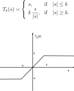
abstract results of Chapter 1. To this aim, for every k ≥ 1, we define the truncation Tk : R → R at height k, defined as

Tk(s) =    s, if |s| ≤ k k s |s|, if |s| ≥ k. (2.16)

Figure 2.1: The function Tk(s)

We will prove the following

Theorem 2.2.1. Assume that conditions (2.2),(2.3),(2.6) hold. Then, for

every (u, η) ∈ epi(J) with J(u) < η, there holds |dGJ|(u, η) = 1.

Moreover, if j(x, −s, −ξ) = j(x, s, ξ) is satisfied, then ∀η > J(0) it results |dZ2GJ|(0, η) = 1.

(40)

Proof. Let (u, η) ∈ epi(J) with J(u) < η and let % > 0. Since Tk(v) tends to v

in H1

0(Ω) as k goes to ∞, there exists δ ∈ (0, 1], δ = δ(ρ), and k ≥ 1, k = k(ρ),

such that k ≥ R (where R is as in (2.6)) and

kTk(v) − vk1,2 < % for every v ∈ B(u, δ). (2.17)

From (2.3) we have

j(x, v, ∇Tk(v)) ≤ α(k)|∇v|2.

On the other hand if v ∈ B(u, δ) then v converges to u for a.e. x ∈ Ω. Indeed, if we take vn ∈ H01(Ω) such that vn converges to u in H01(Ω) then, using the

Sobolev embedding theorem, it immediately follows that vn converges to u

in L2_{(Ω). Hence, up to a subsequence, v}

n converges to u for a.e. x ∈ Ω. The

continuity of j with respect to ξ implies that

j(x, v, ∇Tk(v)) → j(x, u, ∇Tk(u))

for a.e. x ∈ Ω. Thus, up to reducing δ, using the Lebesgue Dominated Convergence Theorem, we get the following inequality

Z Ω j(x, v, ∇Tk(v)) < Z Ω j(x, u, ∇Tk(u)) + ρ. (2.18)

Now, since j(x, u, 0) = 0, and by definition of Tk one has

j(x, u, ∇Tk(u)) =        0 if |u| ≥ k j(x, u, ∇u) if |u| ≤ k .

This implies that

(41)

From (2.18) and (2.19) it follows Z Ω j(x, v, ∇Tk(v)) < Z Ω j(x, u, ∇u) + % (2.20)

for each v ∈ B(u, δ). We now prove that, for every t ∈ [0, δ] and v ∈ B(u, δ), there holds

J((1 − t)v + tTk(v)) ≤ (1 − t)J(v) + t(J(u) + %). (2.21)

We consider the expression

j(x, (1 − t)v + tTk(v), (1 − t)∇v + t∇Tk(v)) − j(x, v, ∇v). (2.22)

Adding and subtracting the quantity j(x, v, (1 − t)∇v + t∇Tk(v)), one has

j(x, (1 − t)v + tTk(v), (1 − t)∇v + t∇Tk(v)) − j(x, v, ∇v)

= j(x, (1 − t)v + tTk(v), (1 − t)∇v + t∇Tk(v)) − j(x, v, (1 − t)∇v + t∇Tk(v))

+j(x, v, (1 − t)∇v + t∇Tk(v)) − j(x, v, ∇v).

From (2.2) we obtain that

j(x, v, (1 − t)∇v + t∇Tk(v)) ≤ (1 − t)j(x, v, ∇v) + tj(x, v, ∇Tk(v)) =

= t(j(x, v, ∇Tk(v)) − j(x, v, ∇v)) + j(x, v, ∇v).

Therefore we have

j(x, v, (1 − t)∇v + t∇Tk(v)) − j(x, v, ∇v)

≤ t(j(x, v, ∇Tk(v)) − j(x, v, ∇v)). (2.23)

Since j(x, s, ξ) is of class C1 _{with respect to the variable s, there exists}

θ ∈ [0, 1] such that

(42)

2.2 A fundamental theorem 31 = tjs(x, v + θt(Tk(v) − v), (1 − t)∇v + t∇Tk(v))(Tk(v) − v). (2.24) We observe that        v(x) + θt(Tk(v(x)) − v(x)) ≥ R if v(x) ≥ k v(x) + θt(Tk(v(x)) − v(x)) ≤ −R if v(x) ≤ −k

Indeed, if v(x) ≥ k then Tk(v) = k, and therefore:

v(x) + θt(Tk(v(x)) − v(x)) = v(x)(1 − θt) + θt · Tk(v(x))

≥ k(1 − θt) + kθt = k ≥ R.

Similarly, if v(x) ≤ −k then Tk(v) = −k, and we get

v(x) + θt(Tk(v(x)) − v(x)) = v(x)(1 − θt) + θt · Tk(v)

≤ −k(1 − θt) − kθt = −k ≤ −R.

Then by (2.6) it follows that, if |v + θt(Tk(v(x)) − v(x))| ≥ R, then

js(x, v + θt(Tk(v) − v), (1 − t)∇v + t∇Tk(v))(v + θt(Tk(v(x)) − v(x))) ≥ 0.

Hence one has        js(x, v + θt(Tk(v) − v), (1 − t)∇v + t∇Tk(v)) ≥ 0 if v(x) ≥ k js(x, v + θt(Tk(v) − v), (1 − t)∇v + t∇Tk(v)) ≤ 0 if v(x) ≤ −k .

(43)

2.2 A fundamental theorem 32 Moreover        Tk(v) − v ≤ 0 if v(x) ≥ k Tk(v) − v ≥ 0 if v(x) ≤ −k

Finally, taking into account that if |v| ≤ k then Tk(v) = v, one has

js(x, v + θt(Tk(v) − v), (1 − t)∇v + t∇Tk(v))(Tk(v) − v) ≤ 0.

Then from (2.24) it follows

j(x, (1 − t)v + tTk(v), (1 − t)∇v + t∇Tk(v))−

j(x, v, (1 − t)∇v + t∇Tk(v)) ≤ 0 (2.25)

Combining (2.23) and (2.25), we deduce that (2.22) becomes

j(x, (1 − t)v + tTk(v), (1 − t)∇v + t∇Tk(v)) − j(x, v, ∇v)

≤ t(j(x, v, ∇Tk(v)) − j(x, v, ∇v))

and therefore, it follows that

j(x, (1−t)v+tTk(v), (1−t)∇v+t∇Tk(v)) ≤ (1−t)j(x, v, ∇v)+tj(x, v, ∇Tk(v)).

Integrating both member of the previous inequality and in view of (2.20), we get (2.21). In order to apply Theorem 1.4.3 we define

H : {v ∈ B(u, δ) : J(v) < η + δ} × [0, δ] → H1 0(Ω)

by setting

H (v, t) = (1 − t)v + tTk(v).

Then, taking into account (2.17) and (2.21), we have:

(44)

2.3 The variational setting 33 and

J(H (v, t)) ≤ (1 − t)J(v) + t(J(u) + ρ).

for v ∈ B(u, δ), J(v) < η + δ and t ∈ [0, δ]. The first assertion now follows from Theorem 1.4.3. Finally, since H (−v, t) = −H (v, t), one also has

|dZ2GJ|(0, η) = 1, whenever j(x, −s, −ξ) = j(x, s, ξ).

2.3 The variational setting

This section regards the relations between |dJ|(u) and the directional deriva-tives of the functional J. Moreover, we will obtain some Brezis-Browder (see [8]) type results. First of all, we make a few observations.

Remark 2.3.1. Hypotheses (2.2) and the right inequality of (2.3) readily imply that there exists a positive increasing function ¯α(|s|) such that

|jξ(x, s, ξ)| ≤ ¯α(|s|)|ξ| (2.26)

for a.e. x ∈ Ω and every (s, ξ) ∈ R × Rn_{. Indeed, from (2.2) one has}

j(x, s, ξ + |ξ|v) ≥ j(x, s, ξ) + jξ(x, s, ξ) · v|ξ|

for every v ∈ Rn _{such that |v| ≤ 1. This and (2.3) yield}

jξ(x, s, ξ) · v|ξ| ≤ α(|s|)|ξ + v|ξ||2− α0|ξ|2

≤ 4α(|s|)|ξ|2_.

From the arbitrariness of v, (2.26) follows. On the other hand, if (2.26) holds, we have |j(x, s, ξ)| ≤ Z ₁ 0 |jξ(x, s, tξ) · ξ|dt ≤ 1 2α(|s|)|ξ|¯ 2_.

As a consequence, it is not restrictive to suppose that the functions in the right-hand side of (2.3) and (2.26) are the same, that is α = ¯α. Notice that,

(45)

2.3 The variational setting 34 Remark 2.3.2. The hypotheses (2.2) and (2.3) imply that,

jξ(x, s, ξ) · ξ ≥ α0|ξ|2. (2.27)

Indeed, we have

0 = j(x, s, 0) ≥ j(x, s, ξ) + jξ(x, s, ξ) · (0 − ξ)

so that inequality (2.27) follows by (2.3).

Now for every u ∈ H1

0(Ω), we define the subspace

Vu = {v ∈ H01(Ω) ∩ L∞(Ω) : u ∈ L∞({x ∈ Ω : v(x) 6= 0})}. (2.28)

It easy to see that Vu is a linear subspace of H01(Ω).

Theorem 2.3.3. For every u ∈ H1

0(Ω) and for every v ∈ H01(Ω) there exists

a sequence {vh} in Vu converging to v in H01(Ω) with −v−(x) ≤ vh(x) ≤ v+(x)

a.e. In particular, Vu is a dense linear subspace of H01(Ω).

Proof. It is enough to treat the case v ∈ H1

0(Ω) ∩ L∞(Ω). Let{ϑh} ⊂ Cc∞(R) such that        ϑh(s) = 1, ∀s ∈ [−h + 1, h − 1] ϑh(s) = 0, ∀s ∈ R \ [−h, h] |ϑ0 h(s)| ≤ 2, ∀s ∈ R

We set vh = (ϑh ◦ u)v; then one has that vh belongs to Vu, vh(x) converges

to v(x), ∇vh(x) converges to ∇v(x) and −v−(x) ≤ vh(x) ≤ v+(x) for a.e.

x ∈ Ω. Moreover, for a.e. x ∈ Ω we have

|ϑh(u(x))v(x)| ≤ |v(x)|,

|ϑ0

(46)

2.3 The variational setting 35

≤ 2|∇u(x)||v(x)| + |∇v(x)|.

By Lebesgue’ s Theorem, vh converges to v in H01(Ω) and the thesis follows.

Since Vu ⊂ Wu ⊂ H01(Ω) and Vu = H01(Ω), then also Wu is dense in H01(Ω).

In the following proposition we study the conditions under which we can compute the directional derivatives of J.

Proposition 2.3.4. Assume that conditions (2.3),(2.5),(2.26) hold. Then

there exists J0_{(u)(v) for every u ∈ dom(J) and v ∈ V}

u. Furthermore, we have

js(x, u, ∇u)v ∈ L1(Ω) and jξ(x, u, ∇u)∇v ∈ L1(Ω)

and J0(u)(v) = Z Ω jξ(x, u, ∇u)∇v + Z Ω js(x, u, ∇u)v.

Proof. Let u ∈ dom(J) and v ∈ Vu. For every t ∈ (0, 1) and for a.e. x ∈ Ω,

we set

F (x, t) = j(x, u(x) + tv(x), ∇u(x) + t∇v(x)).

Since v ∈ Vu using (2.3), it follows that

F (x, t) ≤ α(|u + tv|)|∇u + t∇v|2 ≤ α(kuk∞+ kvk∞)(|∇u| + |∇v|)2

whence F (x, t) ∈ L1_{(Ω). Moreover, it results}

∂F

∂t(x, t) = js(x, u + tv, ∇u + t∇v)v + jξ(x, u + tv, ∇u + t∇v) · ∇v.

From hypotheses (2.5) and (2.26) we get that for every x ∈ Ω with v(x) 6= 0, it results ¯ ¯ ¯ ¯∂F_∂t(x, t) ¯ ¯ ¯

¯ ≤ |v| · β(|u + tv|)|∇u + t∇v|2+ |∇v| · α(|u + tv|)|∇u + t∇v|

≤ kvk∞· β(kuk∞+ kvk∞) · (|∇u| + |∇v|)2

+α(kuk∞+ kvk∞)(|∇u| + |∇v|)|∇v|

Since the function in the right-hand side of the previous inequality belongs to L1_{(Ω), the assertion follows using Lebesgue’s Theorem.}

(47)

2.3 The variational setting 36 In the sequel we will often use the cut-off function H ∈ C∞_{(R) given by}

       H(s) = 1, ∀s ∈ [−1, 1] H(s) = 0, ∀s ∈ R \ [−2, 2] |H0_{(s)| ≤ 2, ∀s ∈ R} (2.29)

Now, we can prove a fundamental inequality regarding the weak slope of J. Proposition 2.3.5. Assume conditions (2.3),(2.5),(2.26). Then we have

|d(J − w)|(u) ≥ sup ½Z Ω jξ(x, u, ∇u)∇v + Z Ω js(x, u, ∇u)v − hw, vi : v ∈ Vu, kvk1,2 ≤ 1 ¾

for every u ∈ dom(J) and every w ∈ H−1_(Ω).

Proof. Taking into account that the weak slope of J − w is a real number in

[0, ∞], it results that if |d(J − w)|(u) = +∞ or if it holds sup ½Z Ω jξ(x, u, ∇u)∇v + Z Ω js(x, u, ∇u)v − hw, vi : v ∈ Vu, kvk1,2 ≤ 1 ¾ = 0, the inequality is satisfied. Otherwise, let u ∈ dom(J) and let η ∈ R+ _be

such that J(u) < η. Moreover, let us consider ¯σ > 0 and ¯v ∈ Vu such that

k¯vk1,2 ≤ 1 and Z Ω jξ(x, u, ∇u)∇¯v + Z Ω js(x, u, ∇u)¯v − hw, ¯vi < −¯σ. (2.30) Let us set vk = H ¡_u k ¢ ¯

v, where H(s) is defined as in (2.29). Since ¯v ∈ Vu we

deduce that vk ∈ Vu for every k ≥ 1. Moreover for a.e. x ∈ Ω we have

|vk(x)| ≤ |¯v(x)|, |∇vk(x)| = ¯ ¯ ¯ ¯H0 µ u(x) k ¶ ∇u(x) k v(x) + H¯ µ u(x) k ¶ ∇¯v(x) ¯ ¯ ¯ ¯ ≤ 2|∇u(x)||¯v(x)| + |∇¯v(x)|.

(48)

2.3 The variational setting 37 By Lebesgue’ s Theorem vk converges to v in H01(Ω). Then, let us fix ε > 0

there exists k0 ≥ 1 such that kvk0 − ¯vk1,2 <

ε 2. Hence we have: kvk0k1,2− k¯vk1,2 < ε 2, that is kvk0k1,2 < k¯vk1,2+ ε 2. This, recalling that k¯vk1,2 ≤ 1, implies

° ° ° °H µ u k0 ¶ ¯ v ° ° ° ° 1,2 < 1 + ε 2. (2.31)

Moreover, by Proposition 2.3.4 we can consider the directional derivatives

J0(u)(vk) = Z Ω jξ(x, u, ∇u)∇vk+ Z Ω js(x, u, ∇u)vk.

In addition, as k goes to infinity, we have

js(x, u(x), ∇u(x))vk(x) → js(x, u(x), ∇u(x))¯v(x) for a.e. x ∈ Ω,

jξ(x, u(x), ∇u(x))∇vk(x) → jξ(x, u(x), ∇u(x))∇¯v(x) for a.e. x ∈ Ω.

Moreover, we get

|js(x, u, ∇u)vk| ≤ |js(x, u, ∇u)¯v|,

|jξ(x, u, ∇u) · ∇vk| ≤ |jξ(x, u, ∇u)||∇¯v| + 2|v||jξ(x, u, ∇u) · ∇u|.

Since v ∈ Vu and by using (2.5) and (2.26), we can apply Lebesgue’s

Domi-nated Covergence Theorem to obtain lim k→∞ Z Ω js(x, u, ∇u)vk = Z Ω js(x, u, ∇u)¯v lim k→∞ Z Ω jξ(x, u, ∇u) · ∇vk = Z Ω jξ(x, u, ∇u) · ∇¯v,

Taking into account (2.30) it follows Z Ω js(x, u, ∇u)H µ u k0 ¶ ¯ v

(49)

2.3 The variational setting 38 + Z Ω jξ(x, u, ∇u)∇ · · H µ u k0 ¶ ¯ v ¸ − ¿ w, H µ u k0 ¶ ¯ v À < −¯σ. (2.32)

In order to apply Proposition 1.2.4, let us consider Jη _{defined as in (1.3).}

Now, we take un ∈ Jη such that un converges to u in H01(Ω) and set

vn= H µ un k0 ¶ ¯ v.

We have that vn converges to H

µ u k0 ¶ ¯ v in H1

0(Ω). Hence let us fixed ε > 0

there exists δ1 > 0 such that, if kun− uk1,2 < δ1, then there holds

° ° ° °vn− H µ u k0 ¶ ¯ v ° ° ° ° 1,2 < ε 2. Therefore kvnk1,2 < ° ° ° °H µ u k0 ¶ ¯ v ° ° ° ° 1,2 +ε 2

and by (2.31) one has kvnk1,2 < 1 + ε. Then we can conclude that

° ° ° °H µ z k0 ¶ ¯ v ° ° ° ° 1,2 < 1 + ε, (2.33)

for every z ∈ B(u, δ1) ∩ Jη. Moreover, note that vn ∈ Vn, so that from

Proposition 2.3.4 we deduce that we can consider J0_(u

n)(vn). From (2.5) and (2.26) it follows |js(x, un, ∇un)vn| ≤ β(2k0)k¯vk∞|∇un|2, |jξ(x, un, ∇un)∇vn| ≤ α(2k0)|∇un| · 2 k0 |∇un|kvk∞+ |∇v| ¸ . Then, we obtain lim n→∞ Z Ω js(x, un, ∇un)vn = Z Ω js(x, u, ∇u)H µ u k0 ¶ ¯ v,

Multiplicity of critical points for some noncoercive functionals

Universit`a della Calabria

Dottorato di Ricerca in Matematica ed Informatica

XIX Ciclo

Tesi di Dottorato (S.S.D. MAT/05 Analisi Matematica)

Multiplicity of critical points for some noncoercive

functionals

Viviana Solferino

Multiplicity of critical points for some noncoercive functionals

Viviana Solferino

Contents

Introduction

Chapter 1

Recalls of nonsmooth critical

point theory

1.1

The weak slope

1.2

The case of lower semicontinuous

func-tionals

1.3

The equivariant case

1.4

The results of nonsmooth analysis

Chapter 2

Unbounded critical points for a

class of lower semicontinuous

functionals

2.1

The main result

2.2

A fundamental theorem

2.3

The variational setting