F
ACOLTÀ DII
NGEGNERIAC
IVILE EI
NDUSTRIALE ______________________DIPARTIMENTO INGEGNERIA CHIMICA,MATERIALI E AMBIENTE
Corso di Dottorato in Ingegneria Elettrica, dei Materiali e delle Nanotecnologie XXXI Ciclo
Tesi di Dottorato:
SPATIO-TEMPORAL VARIABILITY ANALYSIS
OF TERRITORIAL RESISTANCE AND RESILIENCE
TO RISK ASSESSMENT
Dottoranda: Relatori:
Monica Cardarilli Prof.ssa Mara Lombardi
Prof. Giuseppe Raspa
Correlatore:
Geol. Angelo Corazza
2
“There are two days in the year that we can not do anything, yesterday and tomorrow”
3
Abstract
Natural materials, such as soils, are influenced by many factors acting during their formative and evolutionary process: atmospheric agents, erosion and transport phenomena, sedimentation conditions that give soil properties a non-reducible randomness by using sophisticated survey techniques and technologies. This character is reflected not only in the spatial variability of soil properties which differ punctually, but also in their multivariate correlation as function of reciprocal distance.
Cognitive enrichment, offered by the response of soils associated with their spatial variability, implies an increase in the evaluative capacity of contributing causes and potential effects in the field of failure phenomena.
Stability analysis of natural slopes is well suited to stochastic treatment of the uncertainty which characterized landslide risk. In particular, the research activity has been carried out in back-analysis to a slope located in Southern Italy that was subject to repeated phenomena of hydrogeological instability - extended for several kilometres and recently reactivated - applying spatial analysis to the controlling factors and quantifying the hydrogeological susceptibility through unbiased estimators and indicators.
A natural phenomenon, defined as geo-stochastic process, is indeed characterized by interacting variables leading to identifying the most critical areas affected by instability. Through a sensitivity analysis of the local variability as well as a reliability assessment of the time-based scenarios, an improvement of the forecasting content has been obtained. Moreover, the phenomenological characterization will allow to optimize the attribution of the levels of risk to the wide territory involved, supporting decision-making process for intervention priorities as well as the effective allocation of the available resources in social, environmental and economic contexts.
4
Preface
The basis of this research originally stems from my passion for developing methodologies concerning natural hazard analysis and risk assessment.
As the world moves further into disaster mitigation and emergency management trying to reduce the potential consequences in term of affected people, damage to critical infrastructure and disruption of basic services, there is the real need to actively contribute giving global society more tools aiming at increasing territorial resistance and resilience as much as reducing the impact of landslides thought a better understanding of its complex variability.
The case study was assigned for its huge extension and massive reactivations over time causing damages to downstream infrastructures as well as the interruption of mobility systems from and to the areas affected by the landslide events.
Following the recent execution of structural interventions along the landslide body and the numerous studies conducted to date by many authors on the same case study, a specific interest has been raised: how much the landslide hazard has been reduced and which areas are more susceptible towards a residual risk management planning.
The project was undertaken in strong collaboration with the Italian Civil Protection Department (DPC), where I undertook a traineeship in which an extensive investigation and data collection of the assigned case study has been accomplished followed by a field trip to the landslide site.
Furthermore, a second traineeship was conducted at the Joint Research Centre (JRC-Ispra) for reducing natural-hazard impacts on critical infrastructures by applying stochastic approaches and quantitative methodologies.
Finally, as member of the ‘Young Scientists Programme’ of Integrated Research on Disaster Risk (IRDR), the research has acquired a multi-disciplinary character benefiting from a joint network of scientific exchange and professional cooperation.
For these reasons, I would thank you all the supervisors and working groups for their guidance and support during these years without whose cooperation I would not have been able to conduct this research activity.
5
Contents
Abstract ... 3 Preface... 4 Introduction ... 7 Chapter I ... 10The Factor of Safety (FS) ... 10
1.1 Safety in Engineering ... 10
1.2 Slope Stability as Safety Condition... 10
1.3 Probability of Failure ... 12
1.4 Slope Stabilization ... 13
Chapter II ... 16
Characterization of Soil Uncertainty ... 16
2.1 Sources of Soil Uncertainty ... 16
2.2 Soil Uncertainty Assessment ... 20
Chapter III ... 23
Stochastic Modelling of Soil ... 23
3.1 Statistical Analysis of Variability ... 23
3.2 Geostatistical Approach ... 25
3.2.1 Spatial variogram model ... 26
3.2.2 Kriging: spatial prediction method ... 29
3.3 Reliability Approach... 32
3.3.1 Random variables ... 35
3.3.2 Monte Carlo Simulation: random process method ... 36
Chapter IV ... 38
Case Study: the Landslide of Montaguto (AV)... 38
4.1 Earthflow Phenomenon Description ... 38
4.1.1 Geography and historical activity ... 40
4.1.2 Geological and hydrological setting... 42
6 4.1.4 Mitigation measures ... 51 4.2 Soil Characterization ... 53 4.2.1 Data collection ... 55 4.2.2 Categorization of data ... 65 4.2.3 Multivariate analysis ... 71
4.3 Spatial Variability Modelling ... 78
4.3.1 Variograms scales ... 81
4.3.2 Stochastic soil predictions ... 87
4.4 Slope Instability Assessment ... 112
4.4.1 Deterministic slope modelling ... 113
4.4.2 Probabilistic slope failure ... 120
4.4.3 Sensitivity analysis of variability ... 124
4.5 Stochastic Mapping of Slope Instability ... 137
4.5.1 Interventions as conditioning elements: Instability Prediction ... 138
4.5.2 Interventions as conditioning elements: Instability Simulation ... 142
Chapter V ... 144
Conclusions ... 144
References ... 149
Appendix 1 ... 167
Kolmogorov - Smirnov test ... 167
Appendix 2 ... 169
Regression model with interactions ... 169
Appendix 3 ... 171
Statistics and probability distribution of soil properties ... 171
List of Figures ... 175
List of Graphs ... 178
7
Introduction
Worldwide in the last decade, a new vision and collective sensitivity have been affirmed on disaster risk reduction particularly on stability phenomena (St. Cyr, 2005) thanks to institutions and administrations action in territorial planning in which scientific community and research institutes have been providing fundamental support.
Mitigation policy of the impact of hydrogeological events is essentially based on two parallel and coordinated actions: the organization of interventions which guide social response in emergency contexts and the planning of preventive and protective decisional activities in delayed time (UNISDR, 2017a). In particular, satellite observation technologies of natural phenomena are increasing for a more successful outcome of preventive land management (Quanta Technology, 2009) in quiescent conditions, forecasting the potential effects induced on the areas of interest more accurately.
The increasing availability of data, acquired through modern and sophisticated systems and innovative detection processes, has been associated with application methods and elaborated through numerical modeling aimed at assessing extreme events (Rouaiguia and Dahim, 2013).
The use of new technologies, associated with a growing safety demand of society, makes the development of integrated technical and scientific methodologies necessary to guide predictive spatial planning through a reliable assessment of risk in heterogeneous and dynamic contexts such as those deriving from hydrogeological instability conditions (Ferlisi, 2013) with exogenous - often anthropogenic - origin.
Technological progress and technical-scientific knowledge should lead to improve quantitative analysis by carrying out a reliable probabilistic assessment (Li et al., 2013) for characterizing spatial uncertainty and dynamic evolution of potential risk levels. In the same way, this concerns the need to implement a quantitative procedure for the estimation of the variables affecting scenarios in order to reduce risk to a residual value (Bhattacharya, Chowdhury and Metya, 2017).
These are needs that should meet coordinated investments aiming at synergistic activities to forecast catastrophic events particularly in susceptible territorial contexts (Rossi et al., 2010) either in terms of extension or spatial distribution, considering evolution and duration as well. In fact, enrichment and quantitative cognitive improvement offered by soil response as well as evaluative capacity of
8
potential causes and expected effects should be adapted to the fragility of the specific area.
The development of applied research and technologies for mitigating “natural” risk in many countries provides wide and useful tools to achieve a more effective disaster risk reduction (Fisher et al., 2014). The use of joint methodologies deriving from multi-disciplinary fields and integrated application methods, would allow to improve planning and safeguarding activities (Marx and Cornwell, 2001), giving a comprehensive risk assessment for natural hazards.
Landslides are among the most potentially manageable of all natural hazards, given the range of approaches and techniques that are available to reduce the level of hazard. There is much scope to reduce their impacts (UNISDR, 2017b). Landslide hazard is a function of susceptibility, as spatial propensity to landslide activity, and temporal frequency of landslide triggers, and its assessment may be done on local (individual slope), regional, national, continental, or even global scales (UNISDR, 2017a). The most appropriate method in each scale depends on the extent of the study area and on the available data (Nadim, Einstein and Roberds, 2005; Nadim et al., 2006; Corominas and Moya, 2008). In any type of landslide hazard assessment, there is a need to consider topography and other factors that influence the propensity to landslide activity (susceptibility factors), as well as landslide triggering factors (precipitation, earthquakes, human activity).
Climate change increases the susceptibility of surface soil to instability because of abandoned agricultural areas, deforestation and other land-cover modifications. Anthropogenic activities and uncontrolled land-use are other important factors that amplify the uncertainty in landslide hazard assessment (Meusburger et al., 2012).
Disasters may catalyse moments of change in risk management aims, policy and practice. Increasingly, the decision-making processes of the authorities in charge of reducing the risk of landslides and other hazards are moving from “expert” decisions to include the public and other stakeholders (Scolobig, Thompson and Linnerooth-Bayer, 2016).
Further, the Hyogo Framework of Action 2005–2015 and the Sendai Framework for Disaster Risk Reduction 2015–2030 emphasise the importance of improved resilience at national and local community level. The concept of resilience is variously defined but covers the capacity of public, private and civic sectors to withstand disruption, absorb disturbance, act effectively in a crisis, adapt to changing conditions, including climate change, and grow over time (Martin-Breen and Anderies, 2011) (Kervyn et al., 2015).
9
Building resilience not only require accurate hazard estimates that account for spatial distribution, temporal frequency and hazard intensity, but also quantitative assessments of their impacts, as well as the evaluation of current social and cultural structures affecting the territorial vulnerability (Nakileza et al., 2017). This is essential to identify effective adaptation strategies that are cost-effective, technically efficient, culturally acceptable and adapted to the livelihoods of the vulnerable populations.
In this research, a quantitative analysis has been carried out considering the probabilistic distribution of the most influential (Jaksa, 1995) spatial variables identified. In this way may be highlighted the presence of interdependence and potential mutual correlation of the conditioning parameters (Sarma, Krishna and Dey, 2015).
The acquisition of data and territorial information has been performed by considering different geo-environmental elements such as empirical measurements, instrumental monitoring, historical series and statistical databases, integrated to outline a cognitive framework.
A clear advantage is therefore the benefit of a deeper phenomenological knowledge, reorganizing the geo-information to complete implementation of procedures to conduct territorial planning and management as well as coordination of urgent interventions (Cardarilli, Lombardi and Guarascio, 2018).
Common methodologies currently associated with the characterization of instability phenomena of natural soils use semi-probabilistic approaches (Marx and Cornwell, 2001) often neglecting the spatial component. The aleatory uncertainty (Valley, Kaiser and Duff, 2010), belonging to every environmental context, has been recognized as component that may be characterized due to its intrinsic variability, often ignored (F. . Dai, Lee and Ngai, 2002).
To date, spatio-temporal references (Pebesma and Graeler, 2017) concerning mitigation and monitoring are lacking. Planning activities consist of heterogeneous scenarios (Phoon et al., 2006a) and unconditional parametric sequences (Kim and Sitar, 2013) whose predictions do not depend on reliability considerations (Cho, 2013). Essential is therefore the introduction of methodologies which have long been using in mining field - Geostatistics - within hydrogeological context (Meshalkina, 2007).
10
Chapter I
The Factor of Safety (FS)
1.1 Safety in Engineering
The goal of safety is the preservation of existence of an individual or a community (Ferlisi, 2013). Although the term safety may be found in many laws, this does not necessarily mean that the content of the term is clearly defined (Metya, 2013), so many people have a different understanding of the term (Diamantidis et al., 2006).
Some common descriptions are following presented (Proske, 2008):
• Safety is a state in which no disturbance of the mind exists, based on the assumption that no disasters or accidents are impending;
• Safety is a state without threat;
• Safety is a feeling based on the experience that one is not exposed to dangers; • Safety is the certainty of individuals or communities that preventive actions
will function reliably.
Safety requirements and safety concepts have a long history in some technical fields (Fleming and Leveson, 2015) especially concerning natural slope stability (Cheng, 2004).
1.2 Slope Stability as Safety Condition
A slope is a portion of soil which, for its topographic characteristics, may undergo a movement according to the gravity (Duncan, 1999).
Landslides can be triggered by many, sometimes concomitant causes. Seasonal rainfall is generally responsible of shallow erosion or reduction of shear strength (Kim et al., 2004). In addition, landslides may be triggered by anthropic activities such as adding excessive weight above the slope, digging at mid-slope or at the foot (Kim, Jeong and Regueiro, 2012). Often, more than one triggering factor joins together to generate instability over time, which often does not allow a clear reconstruction of phenomenon evolution.
11
Causes Phenomena Possible Reasons
Increase in stresses
Natural actions
Erosion Seismic forces
Water thrusts, Freezing Anthropic actions Excavations
Overloading
Decrease in resistances
Increasing pore water pressure Meteorological events Groundwater excursion Variation of strength parameters Changes in hydraulic conditions Alteration of rocks
Soil degradation (softening, creep)
Table 1 - Causes of soil movement (source: F. Dai, Lee and Ngai, 2002)
The term stability of a slope may be explained as a balance of the shear stresses, induced by the gravity on the mass of soil, to the available soil shear strength before collapsing (Duncan, 1999). In the practice, this equilibrium condition is numerically expressed as Factor of Safety (FS).
FS = Available Soil Shear Strength Equilibrium Shear Stress
The main interest of slope stability is the assessment of FS along the potential failure slip surface where its results the lowest. According to this, a Factor of Safety equal to 1 indicates that the slope is at limit equilibrium; below 1 indicates an unstable slope that theoretically already should have failed, and consequently greater than 1 indicates stability (Duncan, 2000).
Figure 1 - Slope failure mechanism (source: Wyoming State Geological Survey) (1)
12
The conventional safety factor depends on physical model, method of calculation, load conditions and soil parameters. Therefore, all these factors with their level of approximation of slope stability conditions, involve uncertainty in FS computation. Another factor concerns also the ability to find the critical slip surface both in term of geometry and position (F. C. Dai, Lee and Ngai, 2002).
In most cases, the most pronounced sources of uncertainty in a slope stability analysis concern soil strength and groundwater levels; a probabilistic evaluation of soil parameters may help in assessing the Factor of Safety (Zhang, 2010).
1.3 Probability of Failure
Engineers are very familiar with uncertainties especially in natural and environmental contexts. This leads to consider uncertainty in a probabilistic way for representing its randomness (Fallis, 2013).
A Probability Density Function (PDF) may be introduced to model the relative likelihood of a random variable. The PDF describes, in fact, the relative likelihood that the variable has a certain value within a range of potential values.
Since soil strength and applied loads are each subject to uncertainties, they may be considered as random variables as well as the Factor of Safety which results from their joint combination (Johari, Fazeli and Javadi, 2013). Based on the PDF of FS, the application of a probabilistic modelling gives also the distribution of FS values then the likelihood of failure.
Figure 2 - Deterministic and Probabilistic distributions of Load and Strength
(source: Mustaffa, Gelder and Vrijling, 2009)
The advantage of the probability model is that with appropriate considerations and assumptions the PDF extends beyond the information portrayed by the
13
observed data for the specific site, as well as other related factors. Caution must be exercised, however, to ensure the appropriateness of the PDF in representing the site and state of stability (Hsu, 2013).
Figure 3 - Probability of Failure P(FS) (source: Johari and Javadi, 2012)
The relative contribution of different factors in slope failure should be kept in mind when a target probability is being selected (Diamantidis et al., 2006). It makes little sense to reduce the computed probability of failure due to slope stability problems if other triggering causes are not addressed at the same time taking also in account past experiences and further studies performed until nowadays (Valley, Kaiser and Duff, 2010).
1.4 Slope Stabilization
Landslide mitigation generally consists of non-structural and structural activities aiming at reducing the probability of occurrence and/or the impact of landslide event on people and goods at risk (Popescu and Sasahara, 2005).
It is possible to consider a subdivision of stabilization interventions in relation to triggering factors and movement mechanism that each measure addresses (Popescu, 2001):
• Geometrical methods, in which the geometry of the slope profile is modified (slope inclination from the horizontal plane);
• Hydrogeological methods, in which an attempt is made to lower the groundwater level or to reduce the water content of the material by draining elements;
• Chemical methods, which increase the shear strength of the unstable mass by introducing internal slope reinforcements thought additive materials;
14
• Mechanical methods, which introduce active external forces (e.g. anchors, or ground nailing) or passive (e.g. retaining walls, piles or reinforced ground) to counteract the destabilizing forces.
Figure 4 - Drainage system (left) and anchorage grid (right)
(sources: Weinstein Construction Corp and Dywidag systems)
Geometrical modification is the most common method that has been used, usually simple and less costly. The changing of the slope angle from steep slope to a gentler slope may increase the stabilization of slope mainly thought roughening, terracing and rounding. Moreover, the angle is usually supported by grass bonding together with soil. Vegetation has, in fact, a beneficial effect on slope stability by the processes of interception of rainfall, and transpiration of groundwater, thus maintaining drier soils and enabling some reduction in potential peak groundwater pressures.
This type of method does not require heavy load resistance and naturally stabilize the slope with the creepy grass surface which requires minimum maintenance.
Drainage concerns one of the slope failure factors: saturation degree and pore water pressure building up in the subsoil. A drainage system may minimize the instability by reducing the surface water and groundwater level with very effective increases of shear strength.
As a long-term solution, however, it suffers greatly because the drains must be maintained if they are to continue to function (Charles and Bromhead, 2008). In general, this method is very common and used in combination with other methods (Glade, Anderson and Crozier, 2012).
Surface drains may discharge more water, especially during heavy rain to avoid the effects of large amounts of water absorption by the slope.
Retaining structures are generally more expensive. However, due to its flexibility in a constrained site, it is always the most commonly adopted method. The principle of this method is to use earth-retaining structures to resist the
15
downward forces of the soil mass. It also may reduce rainwater infiltration and prevent slope erosion of the slope forming materials.
Over the last several decades, there has been a notable shift forward novel methods such as “internal stabilization” through consolidating additives (lime or concrete), grouting, soil nailing or reinforced grids which increase shear strength. The cost of these remedial measures is considerably lower when compared with the cost of classic structural solutions.
Within the general domain of the structural mitigation measures, they should firstly concern the specific site conditions as well as the economic cost often limited (Song et al., 2014):
• Application of slope; • Purpose of stabilizing; • Time available;
• Accessibility of the site;
• Types of construction equipment; • Cost of repair and maintenance; • Sustainable environmental impact.
The experience shows that while one remedial measure may be dominant, most landslide repairs involve the use of a combination of two or more of the major categories.
However, the success of corrective slope regrading (fill or cut) is determined not merely by size or shape of the alteration, but also by position on the slope (Popescu and Sasahara, 2005).
16
Chapter II
Characterization of Soil Uncertainty
2.1 Sources of Soil Uncertainty
Many variables are involved in slope stability analysis as well as in the evaluation of Factor of Safety. It requires physical data on geologic materials and shear strength parameters (i.e. cohesion and angle of internal friction), pore water pressure, geometry of slope, unit weight, etc.
Soil components may affect locally the slope behaviour and globally the geo-mechanic response but, in addition, they are characterized by variability which leads to uncertainty (Garzón et al., 2015).
The variability associated with soil is uncertain due to many reasons which lead to increasing uncertainty in slope stability as well. The associated uncertainty varies in each analysis and is case specific (Borgonovo, 2007). Soil uncertainties depends mainly on:
• Site topography and stratigraphy; • Geology and geomorphology; • Groundwater level;
• In-situ characteristics; • Properties of materials; • Mechanical behaviour.
Owing to the nature of soil, it is necessary to individuate and evaluate the uncertainties. Concerning slope stability assessment, the sources may be grouped into three main categories (Phoon et al., 2006a), associated with:
• Measurement (laboratory and field investigations);
• Transformation (indirect relations between soil parameters, modelling); • Inherent variability of ground conditions at the site (natural soil processes).
17
Figure 5 - Uncertainty diagram in soil property estimates (source: Phoon and Kulhawy, 1999) The first source of uncertainty arises from the difficulty in measuring soil properties (i.e. geological, hydrogeological, geomechanical etc.). Any measurement involves errors due to equipment, procedural/operator sampling process, testing effects. This uncertainty may be minimised increasing tests’ density, but it is commonly included within the measurement errors (Phoon, 1999).
Properties such as permeability, compressibility, shear strength, in a soil deposit, may show significant variations, even when located within homogeneous layers. On the other hand, in every investigative campaign, the volume of investigated and sampled soil represents a very small portion of the total volume of soil affected, and global behavior assessments must necessarily be made based on limited, often deficient, information (Phoon and Kulhawy, 1999).
The second one is introduced when field or laboratory measurements are transformed into design soil properties by using empirical or other correlation models. The relative contribution of these uncertainties clearly depends on the precision of the applied models (Phoon et al., 2006a).
To date, the focus on technology has made it possible to increase the efficiency of the technical execution of surveys and to reduce the time of data acquisition as well. It has also improved and integrated the best experiences with empirical transformations of different variables characterizing soils.
18
Figure 6 - Uncertainty diagram in geotechnical design process (source: Honjo and Otake, 2011) Collectively, these two sources may be described as data scatter. Two types of uncertainty were identified. The first one was the knowledge or epistemic uncertainty which reflects lack of data, lack of information available about events and processes or lack of understanding real phenomena, reducible perfecting survey instruments and knowledge (Riesch, 2013).
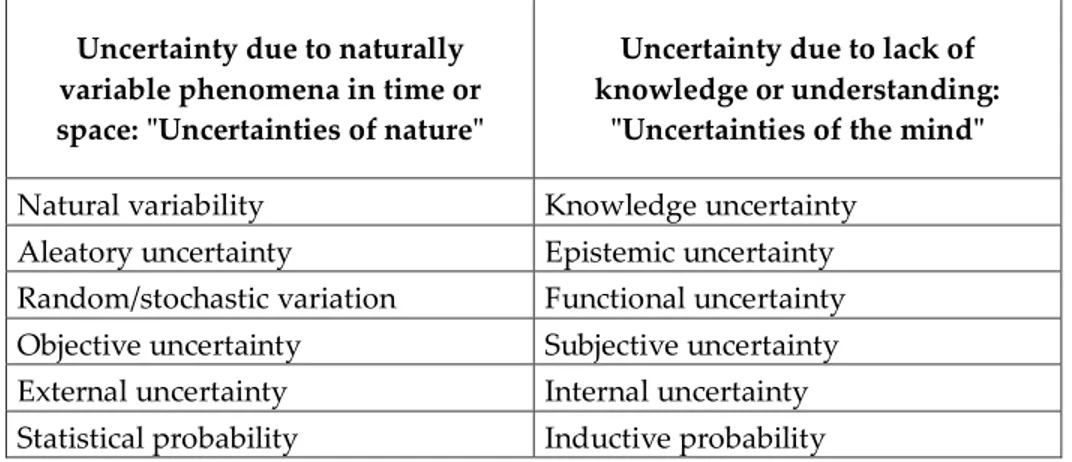
Uncertainty due to naturally variable phenomena in time or space: "Uncertainties of nature"
Uncertainty due to lack of knowledge or understanding:
"Uncertainties of the mind"
Natural variability Knowledge uncertainty Aleatory uncertainty Epistemic uncertainty Random/stochastic variation Functional uncertainty Objective uncertainty Subjective uncertainty External uncertainty Internal uncertainty Statistical probability Inductive probability
Table 2 - Terms used in the literature to describe the duality of meaning for "uncertainty"
(source: Muller, 2013)
The third type of uncertainty governs physical properties due to their composition and complex depositional processes over time which are involved in soil formation. The natural inherent character is unknown to designers and must be deduce from limited and uncertain observations.
The term used to define this third uncertainty is natural or aleatory which means non-reducible (Phoon and Kulhawy, 1996). It represents soil uncertainty over
19
time for phenomena that take place at a single location (temporal variability), or over space for phenomena which take place at different locations but in a single time (spatial variability), or both (spatial-temporal variability) (Phoon et al., 2006a).
The final objective is the reconstruction of the physical model of the territory, basic for any further step of analysis. In fact, the quality of results obtained is strictly connected to the reliability and uncertainty of the source data.
Mac (2014) considers geological data affected by different estimation error depending on the type of data. This estimation error is connected primarily to a certain data dispersion, due mainly to:
• Intrinsic natural variations; • System heterogeneity; • Anisotropy of parameters; • Sampling difficulties; • Noise of natural system; • Calculation system noise.
Therefore, due to the complexity of geological materials, it is important to consider the difficulty of modeling soil. Simplifications and conceptual assumptions are needed to define geotechnical models, trying to be as much effective as possible especially in design practice. The characterization of the reliability degree, however, turns out to be, in some contexts of analysis, indispensable (Johari, Fazeli and Javadi, 2013).
Finally, the factors triggering landslides are, by their nature, subject to a high degree of uncertainty.
Every scale of investigation, characterization and analysis of natural phenomena involves uncertainties that, directly or indirectly, must be considered. In most cases of slope analysis, uncertainty is associated with geotechnical parameters, geotechnical models, frequency, intensity and duration of triggering agents. The importance of different uncertainties depends on size and relevance of the specific site as well as the extension and from the quality of investigations and laboratory tests performed leading to inadequate representativeness of data samples due to time and space limitations. Another source of uncertainty is the temporal variability of parameters such as interstitial water pressure within the slope at different depths and especially along the potential sliding surface. Ideally, we would like to have perfect knowledge of site conditions, but resources are limited. Expenditures must be commensurate with both the scope of design
20
and with the potential consequences of using incomplete and imperfect information in making decisions.
Excellent authors (Vanmarcke, 1980; Rethati, 1989; Christian, Ladd and Baecher, 1994; Lacasse and Nadim, 1996; Jaksa, Kaggwa and Brooker, 1999; Phoon and Kulhawy, 2001; Cassidy, Uzielli and Lacasse, 2008; Bond and Harris, 2008; Griffiths, Huang and Fenton, 2009; among others) focused on the need to develop new methods concerning spatial and temporal variability treatment of soil data which aim at optimizing their usage as well as providing a soil characterization and analysis as reliable as accurate.
2.2 Soil Uncertainty Assessment
It is often convenient in risk and reliability analysis to presume that some part of natural uncertainty is due to randomness. This allows to use probabilistic approaches to bear on a problem that might otherwise be difficult to address, incorporating probabilities of both aleatory and epistemic variability (Sarma, Krishna and Dey, 2015).
It is important to point out that the presumed randomness in this analysis is a part of the models, not part of the site geology. The assumption is not being made that site geology is in some way random: once a formation has been deposited or formed through geological time, the spatial distribution of structure and material properties is fixed (Zêzere et al., 2004).
Probabilistic approach results crucial when evaluating, either at quantitative or qualitative level, hazard and consequences of a calamitous event potentially affecting people, environment, infrastructures, local activities and so on (Zhang, 2010).
A probabilistic approach to studying geotechnical issues offers a systematic way to treat uncertainties, especially in soil stability.
Deterministic slope stability analysis uses single value for each variable to calculate the Factor of Safety without evaluating the probability of failure (Alimonti et al., 2017).
Different approaches try to evaluate soil variability. Relatively to the level of “knowledge” or complexity, they may be applied to the treatment of many problems depending on the relevance of design or, in this case, on the consequences of landslide events.
All methods assume soil parameters as variables that may be expressed as Probability Density Function (PDF). As a result, stochastic approaches, based on probabilistic analysis, provide useful and different information. They are
21
following listed and described according to the level of details provided (Vanmarcke, 1980):
• Semi-probabilistic (Level I); • Probabilistic simplified (Level II); • Probabilistic rigorous (Level III).
The first level proposes a probabilistic approach based on characteristic values of each design variables (resistances and loads), conceived as fractiles of the statistical distributions. The characteristic values (respectively Rk and Ek) are
defined as lower/upper values which minimise safety, considering volume involved, field extension and laboratory investigations, type and number of samples and soil behaviour (Bond and Harris, 2008).
The second level of soil variability evaluation is the probabilistic simplified approach. In this method, FS may be interpreted in terms of probabilities or of suitable safety indices, leading to defining the probability of failure corresponding to FS less than or equal to 1 (Bond and Harris, 2008).
It assumes soil parameters as aleatory variables that may be expressed with PDF curves. An alternative way of presenting the same information is in the form of Cumulative Distribution Function (CDF), which gives the probability of a variable in having value less than or equal to a selected one.
This method attempts to include the effects of soil property variability giving, in addition to fractile, two more values per each uncertain parameter which characterized the PDF: sample mean value () and sample standard deviation () of the probabilistic distribution function, respectively measuring the central tendency of the aleatory variable and its deviation, the average dispersion of the variable from its mean value (Bond and Harris, 2008).
The normal or Gaussian distribution is the most common type of probability distribution function and respects the distribution of many aleatory variables conform to it (Jiang et al., 2014). It is generally used in probabilistic studies in geotechnical engineering unless there are good reasons for selecting different distributions. Typically, variables which arise as a sum of several aleatory effects are normally distributed (Li et al., 2011).
The problem of defining a normal distribution is to estimate the values of the governing parameters which are the true mean and the true standard deviation. Generally, the best estimates for these values are given by the sample mean and standard deviation, determined from a few tests or investigations. Obviously, it is desirable to include as many samples as possible in any set of observations but, in geotechnical engineering, there are serious practical and economic limitations to the amount of data which may be collected.
22
Therefore, this approach provides statistical values of soil parameters to stochastically evaluate soil natural variability. The FS obtained is a curve of probability distribution numerically expressing the probability of failure of slope equilibrium condition (Meyerhof, 1994).
The probabilistic rigorous approach performs probabilistic analysis considering not only measured values but also and especially its arrangement within the volume of soil explored. In fact, the claim of this method consists in providing a comprehensive statistical knowledge of all the variables that influence FS: soil parameters evaluated in three-dimensional contest (Griffiths, Fenton and Tveten, 2002).
Another feature consists in soil inherent variability considered no more random. Based on probabilistic tools currently available, the analyses aim at a complete understanding of soil spatial laws is not feasible yet, remaining a pure theoretical reference. This underlines as the first two approaches are extremely reductive and approximate in soil characterization then in the evaluation of FS (Griffiths, Huang and Fenton, 2009).
23
Chapter III
Stochastic Modelling of Soil
Experience with panels of experts suggests that model uncertainty is among the least tractable issues dealt with. The difficult questions about model uncertainty have to do with underlying assumptions, with conceptualizations of physical processes, and with phenomenological issues. Failure processes involve strongly non-linear behaviours in considerations of time rates and sequences.
3.1 Statistical Analysis of Variability
Different types of mathematical models are built using different assumptions about natural phenomena. These different assumptions lead to different limitations in the applicability of models and specified boundary conditions. Thus, each model has an appropriate usage and scope dictated by the underlying assumptions. As the number of assumptions underlying a model increases, the scope narrows and accuracy and relevance of the model decreases (Hsu, 2013).
In natural science, quantitative methods represent the systematic empirical investigation of observable phenomena via statistical, mathematical, or computational techniques. They aim at developing and applying mathematical approach pertaining to natural phenomena, such as slope instability, by including (Huang et al., 2013):
• The generation of models, theories and hypotheses;
• The development of instruments and methods for measurement;
• Experimental control and manipulation of variables;
• Collection of empirical data;
• Modelling and analysis of data.
Quantitative research is often contrasted with qualitative approach, which purports to be focused more on discovering underlying meanings and patterns of relationships (Lari, Frattini and Crosta, 2014), including classifications of types of phenomena and entities without involving numerical expression of quantitative relationships of data and observations.
24 Hazard Assessment
Methods
Qualitative methods (Knowledge driven)
Field analysis Inventory mapping
Index or parameter methods
Combination or overlay of index maps Logical analytical models Quantitative methods (Data driven) Statistical analysis Bivariate statistical analysis Multivariate statistical analysis Mechanistic approaches Deterministic analysis Probabilistic analysis Neural network analysis
Table 3 - Scheme of evaluation methodologies (source: Aleotti and Chowdhury, 1999) Statistical models are the most widely used branch of mathematics in quantitative research. In particular, multivariate statistics starts with studies on causal and interacting relationships by evaluating factors that influence landslide phenomena while controlling other variables relevant to obtain experimental frequency and distribution of outcomes in failure regions.
Empirical relationships and mutual correlations may be examined between any combination of continuous and categorical variables by using some form of general linear model, non-linear model, or by using factor analysis (Pinheiro et
al., 2018).
Generally, in this context, to simplify analyses, analytical and transformation models are used to interpret results of site investigation using simplified assumptions and approximations. But, due to the complexity of soil formation and depositional processes, soil behaviour is seldom homogeneous (Svensson, 2014). In addition, the assessment of slope stability is based on approaches based on average/low/high values of soil properties, which may reduce the realistic content of the analyses carried out (Wang, Hwang, Luo, et al., 2013).
Geologic anomalies, inherent spatial variability of soil properties, scarcity of representative data, changing environmental conditions, unexpected failure mechanisms, simplifications and approximations adopted in geotechnical models, as well as human factors (Diamantidis et al., 2006) in stability assessment, are all factors contributing to uncertainty.
Soil components and their properties are inherently variable from one location to another in a three-dimensional space, due mainly to complex processes and effects which influence their formation (Lombardi, Cardarilli and Raspa, 2017).
25
Therefore, the evaluation of the role of uncertainty necessarily requires the implementation of stochastic methods more accurate (Li et al., 2011).
3.2 Geostatistical Approach
The presence of such a spatial variability is the pre-requisite for the application of Geostatistics and its description is a preliminary step towards spatial prediction (Pebesma and Graeler, 2017). Geostatistics is a mathematical discipline which focuses on a limited number of statistical techniques to quantify, model and estimate the spatial variability of sparse sample data (Meshalkina, 2007). Therefore, it may allow to verify whether the simplified models and hypotheses of soil behaviour, used in the conventional approaches, are well-fitting (Valley, Kaiser and Duff, 2010).
Matheron (1963) stated that the model of spatial variation reflects an inherently random process that has generated the site. Nonetheless, it is convenient to structure the models as if some fraction of the uncertainty we deal with has to do with irreducible randomness and then to use statistical methods to draw inferences about the models applied to that natural variability.
Figure 7 - Variability of soil profile (source: Honjo and Otake, 2011)
Before introducing geostatistical analysis, the concept of regionalised aleatory variable (AV) and Aleatory Function (AF) must be introduced (Matheron, 1963). An AV is a variable that may assume multiple values and whose values are randomly generated according to some probabilistic mechanism. The AV Z(x) is also information-dependent, in the sense that its probability distribution changes as more data about the un-sampled value z(x) become available.
26
The regionalised value z(xo) at the specific location xo is one realization of the AV
Z(xo), which is itself a member of the infinite family of aleatory variables.
Therefore, the RV measured at each point is one of the possible results of the Aleatory Function: RV is a realization of AF.
This set of functions, given by the spatial nature of the phenomenon, represents the spatial law of AF Z(x).
Figure 8 - Description of Aleatory Function in S domain (source: Kasmaeeyazdi et al., 2018)
3.2.1 Spatial variogram model
It is the most common function of Geostatistics, used mainly in applications for characterizing spatial variability of regionalised phenomena (Matheron, 1973).
The variogram is defined as the variance of the increment:
[Z(x1) - Z(x2)]
It is written as:
2γ(x1,x2) = Var [Z(x1) − Z(x2)]
The function γ(x1,x2) is then the semi-variogram.
In particular, weak stationarity models are based on the following two hypotheses: E[Z(x)] = E[Z(x+h)] = m Var[Z(x+h)-Z(x)] = 2γ(h) with γ(h) = C(0)-C(h) (2) (3) (4) (5)
27
which respectively mean: constant average value in the whole domain and covariance function invariant by translation. Therefore, the semi-variogram is dependent only on h.
Figure 9 - Schematization of S domain and xi values (source: Famulari, 2013)
Semi-variogram is the best way to describe spatial correlation for which data at two locations are correlated as function of their distance. It is usually defined
autocorrelation or correlation length because referred to the correlation of a single
variable over space (Matheron, 1963).
Generally, the variance changes when the space between pairs of sampled points increases, so near samples tend to be alike. For large spacing, experimental variogram sometimes reaches - or tends asymptotically to - a constant value (sill). It corresponds to the maximum semi-variance and represents the variability in the absence of spatial dependence (Guarascio and Turchi, 1977).
The distance after which variogram reaches the sill is the range and corresponds to the distance at which there is no evidence of spatial dependence. In case sill is only reached asymptotically, range is arbitrarily defined as the distance at which 95% of the sill is reached (Matheron, 1973).
The behaviour at very detailed scale, near the origin of the variogram, is very meaningful as it indicates the type of continuity of the regionalised variable. Though the value of the variogram for h = 0 is strictly 0, several factors, such as sampling error, short scale variability or geological structures with correlation ranges shorter than the sampling resolution (Meshalkina, 2007), may cause sample values separated by extremely small distances to be quite dissimilar. This causes a discontinuity at the origin of the variogram, which means that the values of the variable change abruptly at the scale of detail. For historical reasons, this type of variogram behaviour is called nugget effect. It represents the variability at a point that cannot be explained by spatial structure (Matheron, 1963).
28
Figure 10 - Variogram parameters and function (source: Loots, Planque and Koubbi, 2010) In Geostatistics, spatial patterns are usually described by using experimental variogram which measures the spatial dependence (correlation) between measurements, separated by h displacement (lag distance). The variogram is estimated from available values at sample points so it represents the degree of continuity of the soil property at different locations. In nature, generally, the values of a soil property at two close points are more likely similar than those far away from each other (Sidler, Prof and Holliger, 2003).
The description of spatial patterns is rarely a goal. Generally, there is the need to quantify spatial dependence for predicting soil properties at un-sampled locations. Therefore, it is necessary to fit a theoretical function which describes the empirical variogram of the spatial variability of sampled points as well as possible (Jaksa, 1995).
29
Relatively to spatial analysis there is isotropy when the variogram depends on separation distance h between points instead of directional component (Matheron, 1973). If spatial correlation depends on spatial direction (angular direction), then the spatial process assumes anisotropic correlation. This is a common case in most cases concerning soil properties, due to sedimentation (Pebesma and Graeler, 2017) which often gives a preferential layers’ orientation (the direction of maximum continuity will most likely be parallel to stratigraphy).
Figure 12 - Anisotropy characteristics and discretization (source: spatial-analyst.net)
3.2.2 Kriging: spatial prediction method
A problem common in site characterization is interpolating among spatial observations to estimate soil or rock properties (Sidler, Prof and Holliger, 2003) at specific locations where they have not been observed.
The main application of Geostatistics is the estimation and mapping of spatial soil properties in the un-sampled areas.
The most obvious way to proceed for spatial prediction at un-sampled locations is simply to take an average of the sample values available and assume that it gives a reasonable prediction at all locations in the region of interest. However, if it is known that the variable of interest tends to be spatially correlated, it would make sense to use a weighted average, with measurements at sampled locations that are nearer to the un-sampled location being given more weight (Matheron, 1963).
Kriging has been defined by Olea (2009) as “a collection of generalised linear regression techniques for minimising an estimation variance defined from a prior model for a covariance”. Kriging is just a generic name for a family of generalised
30
linear (least-squares) regression algorithms used to define the optimal weighting of measurements points in order to obtain a spatial prediction as much representative as possible at all un-sampled locations (Functions and Geostatistics, 1991). In Kriging the Euclidean distance is replaced by the statistical distance, which depends on the variogram model assumed (Matheron, 1973).
Kriging belongs to the category of stochastic methods, since it is assumed that measurements, both actual and potential, constitute a single realization of an aleatory (stochastic) process. One advantage of this assumption (Meshalkina, 2007) is that measures of uncertainty may be defined and hence, weights may be determined to minimise the measure of uncertainty. Indeed, much of the advantage of using geostatistical procedures, such as Kriging, lies not just in the point and block estimates they provide, but in the information concerning uncertainty associated with these estimates (Zhang et al., 2013).
Kriging fits a mathematical function to a specified number of points, or all points within a specified radius, to determine the output value per each location. Kriging is a multistep process, it includes exploratory statistical analysis of data, variogram modelling, creating a surface and (optionally) exploring the variance surface (Matheron, 1973).
Oliver and Webster (2014) detailed the following key steps involved in Kriging method of geostatistical estimation:
• A structural study defining the semi-variogram;
• Selection of samples to be used in evaluating the elements; • Calculation of the Kriging system of equations;
• Solution of the equations to obtain optimal weights;
• Use of results to calculate the estimates and the associated estimation variance.
Kriging weights the surrounding measured values for deriving a prediction of un-measured locations (Matheron, 1963). The general formula, applied to original data, consists of a weighted sum of the data:
Z*(x0)= ∑ λi n
i=1
Z(xi)
where:
Z*(xo) = the predicted value at xo location (Kriging estimation);
Z(xi) = the measured value at ith location;
λi = the unknown weight for the measured value at ith location;
31 n = the number of measured values.
In Kriging, weights are based not only on Euclidean distance between measured points and prediction locations, but also on the overall spatial arrangement among observed points. These optimal weights depend, in fact, on the spatial arrangement and autocorrelation quantified (Functions and Geostatistics, 1991).
Figure 13 - Spatial prediction between unsampled point (red) and measured values (black)
(source: resources.esri.com)
The Kriging estimation is the best linear unbiased estimator (Viscarra Rossel et al., 2010) of the Z(x) if the properties in Table 4 are hold.
Estimator
property Definition
Unbiasedness The expected value of Z(x) over all ways the sample might have been realized from the parent population equals the parameter to be estimated Consistency Z(x) converges to the parameter to be estimated
Efficiency The variance of the sampling distribution of Z(x) is minimum
Sufficiency The estimator Z(x) makes maximal use of the information contained in the sample observations
Robustness The statistical properties of Z(x) in relation to the parameter to be estimated are not sensitive to deviations from the assumed underlying PDF of Z
Table 4 - Properties of statistical estimators (source: Sigua and Hudnall, 2008)
Kriging is very popular in numerous scientific fields because its estimates are unbiased and have a minimum variance. Furthermore, this interpolation method may estimate errors associated with each prediction and its correctness, meaning that in a sampled point the estimated value is equal to the observed one, then the mean estimation error is null (Matheron, 1963). In this way Kriging provides also
32
the minimum estimation variance of errors, for which it is defined an accurate method (Matheron, 1973).
It appears evident that Kriging variance, as measure of precision, relies on the correctness of the theoretical variogram model assumed (Kasmaeeyazdi et al., 2018). However (Sidler, Prof and Holliger, 2003):
• As with any method, if the assumptions do not hold, Kriging interpolation might be not representative of data measurements;
• There might be better non-linear and/or biased methods;
• No properties are guaranteed, when the wrong variogram is used. However typically a 'good' interpolation is still achieved;
• Best is not necessarily good: e.g. in case of no spatial dependence, Kriging interpolation is only as good as the arithmetic mean;
• Kriging provides a measure of precision. However, this measure relies on the correctness of the variogram.
Different Kriging methods for calculating spatial weights may be applied. Classical methods are (Oliver and Webster, 2014):
• Simple Kriging, it assumes stationarity of the first moment over the entire domain with a known zero mean;
• Ordinary Kriging, which assumes constant the unknown mean only over the neighbourhood of xo;
• Universal Kriging, assuming a general polynomial trend model;
• Indicator Kriging, which uses indicator functions instead of the process itself, in order to estimate transition probabilities;
• Disjunctive Kriging, it is a nonlinear generalisation of Kriging;
• Lognormal Kriging, which interpolates positive data by means of logarithms.
Concerning phenomena in which the input is uncertain, also Reliability-based theory deals with stochastic modelling (Jiang et al., 2014).
3.3 Reliability Approach
Reliability approach more widely deals with the estimation, prevention and management of engineering uncertainty and risks of failure (Huang et al., 2013), understanding reliability of parameters and/or system.
Reliability is generally defined as the probability that a component will perform its intended function during a specified period of time under stated conditions (Wu et al., 2013).
33
To combine the concept of reliability and to retain the advance of convenience for use like the conventional method of Safety Factor, the concept of safety factor of reliability is introduced.
Concerning FS, reliability approach attempts to account explicitly for uncertainties in load and strength and their probability distribution (Kim and Sitar, 2013).
Figure 14 - Three-dimensional joint density function f(R,S)
(source: risk-reliability.uniandes.edu.co)
Reliability analysis deals with the relation between the loads a system must carry and its ability to carry those loads. Both the loads (S) and the resistance (R) may be uncertain, so the result of their interaction is also uncertain (Wu, 2013). It is common to express reliability in the form of Reliability Index (β), which may be related to Probability of Failure (pf).
Failure occurs when FS < 1, and the Reliability Index is defined by (Belabed and Benyaghla, 2011):
pf= P[FS < 1] = ϕ(−β) β =
μFS− 1 σFS
β is approximately the ratio of the natural logarithm of the mean FS (which is approximately equal to the ratio of mean resistance over mean load) to the coefficient of variation (COV) of FS (Phoon and Kulhawy, 1999).
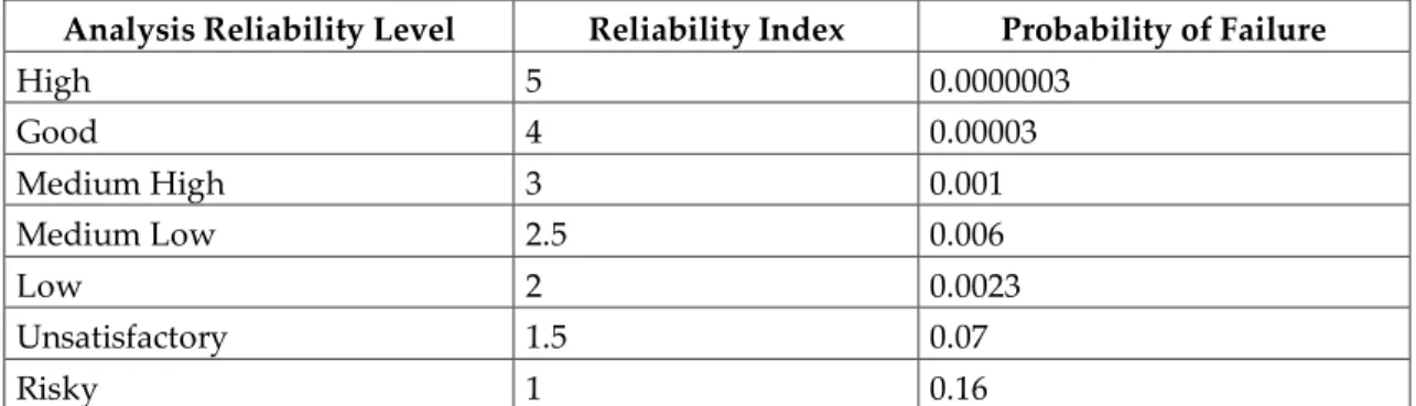
A large value of β represents a higher reliability or smaller probability of failure (Usace, 2006). The reliability level associated with a Reliability Index β is approximately given by the Standard Normal Probability Distribution ϕ, evaluated at β, from Table 5.
34
Analysis Reliability Level Reliability Index Probability of Failure
High 5 0.0000003 Good 4 0.00003 Medium High 3 0.001 Medium Low 2.5 0.006 Low 2 0.0023 Unsatisfactory 1.5 0.07 Risky 1 0.16
Table 5 - Typical values of the Reliability Index and Probability of Failure
(source: Usace, 2006)
Figure 15 - Probability of exceedance (source: daad.wb.tu-harburg.de)
β index thus expresses the stability condition of a slope; if two slopes have the same FS, with different Reliability Index, they have different Probability of Failure (Manoj, 2016). Therefore, in order to calculate the probability of failure it is necessary to hypothesize, or however to know, the probability distribution of FS (Katade and Katsuki, 2009).
There are several methods in literature for assessing β and pf, each having
advantages and disadvantages (Low, 2003). Among the most widely used there are (Belabed and Benyaghla, 2011):
35
• The First Order Second Moment (FOSM) method. This method uses the first terms of a Taylor series expansion of the performance function to estimate the expected value and variance of the performance function. It is called a second moment method because the variance is a form of the second moment and is the highest order statistical result used in the analysis.
• The Second Order Second Moment (SOSM) method. This technique uses the terms in the Taylor series up to the second order. The computational complexity is greater, and the improvement in accuracy is not always worth the extra computational effort.
• The Point Estimate method. Rosenblueth (1975) proposed a simple and elegant method of obtaining the moments of the performance function by evaluating the performance function at a set of specifically chosen discrete points.
• The Hasofer–Lind method or FORM. Hasofer and Lind (1974) proposed an improvement on the FOSM method based on a geometric interpretation of the reliability index as a measure of the distance in dimensionless space between the peak of the multivariate distribution of the uncertain parameters and a function defining the failure condition. This method usually requires iteration in addition to the evaluations at 2N points.
• Monte Carlo Simulation (van Slyke, 1963). In this approach the analyst creates a large number of sets of randomly generated values for the uncertain parameters and computes the performance function for each set. The statistics of the resulting set of values of the function may be computed and β or pf
calculated directly.
The conventional safety factor depends on the physical model (Bowles, 1979), the method of calculation, and most importantly, on the choice of soil parameters. The uncertainty level associated with the resistance and load is not explicitly considered. Consequently, inconsistency is likely to exist among engineers and between applications for the same engineer. The use of a reliability index β may provide significant improvement over the use of the traditional design safety factor in measuring the reliability component (Abbaszadeh et al., 2011).
3.3.1 Random variables
A random process model describes the generating mechanism of a physical phenomenon in probabilistic terms, from which is described the theoretically “correct” stochastic behavior of the phenomenon (Li et al., 2011). This contrasts with an empirical model that simply fits a convenient, smooth analytical function to observed data with no theoretical basis for choosing the particular function.
36
A random variable is a mathematical model to represent a quantity that varies (Johari, Fazeli and Javadi, 2013). Specifically, a random variable model describes the possible values that the quantity may take on and the respective probabilities for each of these values (Huang et al., 2013).
A probability is associated with the event that a random variable will have a given value. Random variables for each calculation are needed from a sample of random values (Hsu, 2013) which are based on the selected PDF which well fits the variable. Although these PDFs may take on any shape, normal, lognormal, beta and uniform distributions are among the most favored for analysis (Low, 2003).
The Normal distribution (also known as the Gaussian distribution) is the classic bell-shaped curve that arises frequently in datasets concerning geotechnical aspects and are used to estimate the PDF of FS. Thus, for uncertainties such as the average soil strength with random variations, the Normal pdf is an appropriate model (Papaioannou and Straub, 2012).
In many cases, there are physical considerations that suggest appropriate forms for the probability distribution function of an uncertain quantity. In such cases (Griffiths, Huang and Fenton, 2009) there may be available from which to construct a function cogent reasons for favoring one distributional form over another, no matter the behavior of limited numbers of observed data (Valley, Kaiser and Duff, 2010).
Much work in probability theory involves manipulating functions of random variables (Griffiths, Fenton and Tveten, 2002). If some set of random variables has known distributions, it is desired to find the distribution or the parameters of the distribution of a function of the random variables useful in generating random Normal variables for Monte Carlo Simulation (Danka, 2011).
3.3.2 Monte Carlo Simulation: random process method
Any simulation releasing on random numbers requires that there is some way to generate the random numbers (EPA, 1997). Statisticians have developed a set of criteria that must be satisfied by a sequence of random numbers. The value of any number in the sequence must be statistically independent of the other numbers (Hsu, 2013).
Monte Carlo technique may be applied to a wide variety of problems employed to study both stochastic and deterministic systems. This method involves random behavior and a number of algorithms are available for generating random Monte
37
Carlo samples from different types of input probability distributions (Harrison, 2010).
The Monte Carlo method is particularly effective when the process is strongly non-linear or involves many uncertain inputs, which may be distributed differently (Enevoldsen and Sørensen, 1994). To perform such a study, it generates a random value for each uncertain variable and performs the calculations necessary to yield a solution for that set of values. This gives one sample of the process. From a set of response realizations, it gives a picture of the response distribution from which probability estimates may be derived (Wu et al., 1997).
The method has the advantage of conceptual simplicity, but it may require a large set of values of the performance function to obtain adequate accuracy. The major disadvantage is that it may converge slowly so it requires a large number of trials directed at either reducing error in sampling process or achieving a desired accuracy. Accurate Monte Carlo simulation depends also on reliable random numbers (Carlo and Galvan, 1992).
Furthermore, the method does not give insight into the relative contributions of the uncertain parameters that is obtained from other methods (Harrison, 2010), each run gives one sample of the stochastic process.
In slope stability context, Monte Carlo simulation produces a distribution of Factor of Safety rather than a single value (Belabed and Benyaghla, 2011). The results of a traditional analysis, using a single value for each input parameter may be compared to the distribution from the Monte Carlo simulation to determine the level of conservatism associated with the conventional design (Danka, 2011). By this procedure, values of the component variables are randomly generated according to their respective PDFs. By repeating this process many times, the Probability of Failure may be estimated by the proportion of times that FS is less than one (EPA, 1997). The estimate is reasonably accurate only if the number of simulations is large; also, the smaller the probability of failure, the larger the number of simulations that will be required (Gustafsson et al., 2012).
38
Chapter IV
Case Study: the Landslide of Montaguto (AV)
4.1 Earthflow Phenomenon Description
Earth flows are among the most common mass-movement phenomena in nature (Keefer, D.K.; Johnson, 1983).
In Italy, earth flows affect large areas of the Apennine range and are widespread where clay-rich, geologically complex formations outcrop (Del Prete and Guadagno, 1988; Martino, Moscatelli and Scarascia Mugnozza, 2004; Bertolini and Pizziolo, 2008; Revellino et al., 2010). Most of them are reactivations of ancient earth flow deposits; only few events are completely new activations (Martino and Scarascia Mugnozza, 2005; Revellino et al., 2010).
Active earth flows generally manifest a seasonal and long-term activity pattern related to a regional climate pattern (Coe, 2012; Handwerger, Roering and Schmidt, 2013) with a higher susceptibility to movement, in the form of local landslides or major reactivations.
Earth flow response to rainfall or snowmelt, in terms of velocity fluctuations, is often delayed, and in several cases, long periods of cumulated precipitation are required to trigger a reactivation (Kelsey, 1978; Iverson, 1986; Iverson and Major, 1987).
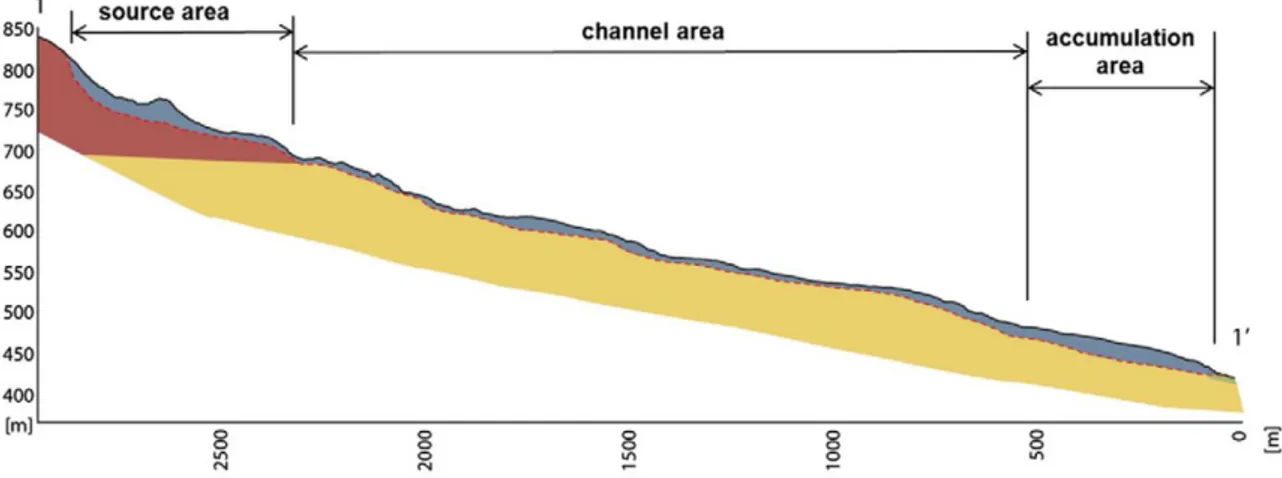
Earth flows are generally identified by an upslope crescent-shaped or basin-shaped scar that is the source area, a loaf-basin-shaped bulging toe that has a long narrow tongue- or teardrop-shaped form (Rengers, 1973; Keefer, D.K.; Johnson, 1983; Bovis, 1985; Cruden and Varnes, 1996; Baum, Savage and Wasowski, 2003; Parise, 2003). Earth flow has characteristic features that make it recognizable on the basis of morphological observation (Keefer, D.K.; Johnson, 1983; Fleming, Baum and Giardino, 1999; Parise, 2003; Zaugg et al., 2016).
The length of an earth flow is commonly greater than its width and its width is greater than its depth.
39
Figure 16 - Earthflow landslide representation diagram (source: Keefer, D.K.; Johnson, 1983) Some authors observed that weak, low-permeability clay layers, characterizing the basal and lateral shear zones of some earth flows, might effectively isolate the earth flow from adjacent ground. This mechanical and hydrological isolation contributes to the persistent instability of earth flows (Baum, R. L, Reid, M. E., 2000).
Shear strength of the clay layer tends to be significantly lower than both the landslide materials and adjacent ground, helping to perpetuate movement on relatively gentle slopes. The presence of the clay layer causes the landslide to retain water (Habibnezhad, 2014).
The term Earthflow was used by many authors (Cascini et al., 2012; Guerriero et
al., 2013; Ferrigno et al., 2017; Bellanova et al., 2018) to describe the Montaguto
slope failure because it is composed of predominantly fine-grained material and has a flow-like surface morphology (Keefer, D.K.; Johnson, 1983; Cruden and Varnes, 1996; Hungr, Leroueil and Picarelli, 2014). However, most movement of Montaguto earth flow takes place by sliding along discrete shear surfaces (Guerriero, Revellino, Coe, et al., 2013). The association of the Montaguto landslide with Earth flow phenomenon will be described in more detail afterwards.