Universit`a degli Studi di Roma Tre
Scuola Dottorale in Scienze Matematiche e Fisiche
Dottorato di Ricerca in Fisica - XXV Ciclo
Measurement of η-meson production in γγ
interactions and Γ
(
η
→
γγ
)
with the KLOE
detector
Thesis submitted to obtain the degree of
”Dottore di Ricerca“ - Doctor Philosophiae
PhD in Physics
Cecilia Taccini
And sure any he has it’s all beside the mark.
-Contents
Introduction 1
1 Mesons in the quark model 3
1.1 The quark model . . . 3
1.2 Mesons mixing . . . 5
1.3 γγcoupling of mesons . . . 6
1.4 Scalar mesons . . . 8
2 Photon-photon interactions 9 2.1 Physics with two photons . . . 9
2.2 Kinematics and cross section of γγ reactions . . . . 11
2.3 Approximations for the cross section formula . . . 12
2.4 Resonance production in γγ interactions . . . . 14
2.5 Tagging of the photons . . . 15
2.6 Form factors in meson-photon-photon transitions . . . 15
2.7 Measurements of radiative widths of mesons . . . 19
3 The KLOE experiment at DAΦNE 21 3.1 The collider DAΦNE . . . 21
3.2 The KLOE detector . . . 22
3.2.1 The drift chamber . . . 23
3.2.2 The electromagnetic calorimeter . . . 25
3.2.3 The quadrupole calorimeters . . . 28
3.2.4 The trigger system . . . 29
3.2.5 Data acquisition . . . 31
3.3 Data reconstruction . . . 31
3.3.1 Cluster reconstruction . . . 31
3.3.2 Track reconstruction . . . 32
3.3.3 Track-to-cluster association . . . 33
4 Data and background sample 35 4.1 Data sample and preselection filter . . . 35
5 Cross section fore+e−→e+e−η with η→π+π−π0 39
5.1 Event selection . . . 39
5.2 Background rejection . . . 39
5.2.1 Photon pairing . . . 40
5.2.2 Kinematic fit . . . 40
5.2.3 Track identification and rejection of the QED background . . . 42
5.2.4 Time and energy quality cuts . . . 45
5.3 Selection efficiency for signal and backgrounds . . . 52
5.4 Cross section evaluation . . . 54
5.4.1 Estimates of background yields from a control region . . . 60
5.5 Evaluation of the systematic uncertainties . . . 63
6 Cross section fore+e−→e+e−η with η→π0π0π0 65 6.1 Event selection . . . 65
6.2 Background rejection . . . 65
6.2.1 Photon pairing . . . 66
6.2.2 Kinematic fit . . . 67
6.2.3 Cut on the energy of the most energetic photon . . . 68
6.2.4 Cut on the 6γ invariant mass . . . . 70
6.3 Selection efficiency for signal and backgrounds . . . 71
6.4 Cross section evaluation . . . 72
6.5 Evaluation of the systematic uncertainties . . . 76
7 Combination of the two cross section values 79 8 Extraction of the partial width Γ(η→γγ) 81 9 Measurement of the cross section fore+e−→ηγ 85 9.1 Event selection . . . 85
9.2 Background rejection . . . 85
9.2.1 Photon pairing . . . 86
9.2.2 Kinematic fit . . . 86
9.2.3 Track identification and rejection of the QED background . . . 87
9.2.4 Cut on the sum of the photon energies . . . 88
9.2.5 Cut on the sum of the track momenta . . . 88
9.3 Selection efficiency for signal and backgrounds . . . 97
9.4 Cross section evaluation . . . 97
9.5 Evaluation of the systematic uncertainties . . . 98
Conclusions 105
Contents
B Energy scale correction 109
B.1 e+e−→ KSKL . . . 109
B.2 e+e−→ ηγ→3π0γ. . . 111
C The Lagrange Multipliers method 113
C.1 The Least-Squares method . . . 113 C.2 Fitting with constraints: Largange Multipliers . . . 114
D The 2-dimensional fit 117
Introduction
Photon-photon interactions are forbidden in classical electrodynamics. According to Maxwell’s linear equations electromagnetic waves cross each other without any disturbance. In quantum electrodynamics (QED), however, the uncertainty principle allows a photon of energy Eγ to
fluctuate into states of charged particle pairs with mass mpair and lifetime ∆t ≈ 2Eγ/m2pair,
and photon-photon scattering becomes possible due to the interaction of the intermediate par-ticles. The cross section for photon-photon interactions is of the order α4, but increases with the beam energy E like(logE/me)2, and therefore already dominates over the O(α2)e+e−
an-nihilation process for beam energies of a few GeV. Experimentally it is difficult to collide high energy photon beams. A simple way of avoiding this problem is to use virtual particles, e.g., the quantum fluctuations of an electron into an electron-photon state. This is done at electron and positron colliders. In the basic diagram of photon-photon reactions both the incoming e+ and e−radiate a photon, predominantly at small angles and with small energies, and the two photons produce the final state X. Photon-photon production of neutral mesons provides basic information on their internal structure. The strength of the coupling, measured by the partial decay width Γ(X → γγ), is related to the quark content of the meson and gives information on the relations between the hadronic state and its q ¯q representation. The measurement of the radiative width of pseudoscalar mesons is indeed a crucial input for the determination of the pseudoscalar mixing angle and for testing the valence gluon content in the η′ wavefunction. Moreover, a precise study of the form factors of the transition γγ∗ → X, where one photon is
off-shell and the other is real, is of particular interest in evaluating the light-by-light contribu-tion to the anomalous magnetic moment of the muon.
Photon-photon interactions in electron-positron colliders were pioneered in the 1970s at ADONE in Frascati and since then have been used to study the production of hadrons in almost all e+e−
colliders in a variety of conditions in low- and high-q2processes. In particular, measurements
of the γγ partial width of η and η′ mesons have been done measuring the e+e− → e+e−η(η′)
cross section.
This thesis is focused on the measurement of the cross section e+e−→e+e−ηand the extraction of the partial width Γ(η → γγ)with the KLOE detector at the φ-factory DAΦNE. DAΦNE is an e+e−collider that operates at the mass of the φ resonance, 1020 MeV. The measurement is done with off-peak data, at√s = 1 GeV, to reduce the large background from φ decays, and with an integrated luminosity of about 240 pb−1. The final state e+ and e− are not detected, being emitted with high probability in the forward directions, outside the acceptance of the
detector. The production of the η meson is identified in two decay modes, η → π+π−π0 and
η → π0π0π0, that exploit in a complementary way the tracking and calorimeter of the detec-tor. The most relevant background for both measurements is the radiative process e+e−→ ηγ
when the monochromatic photon is emitted at small polar angles and escapes detection. The cross section for e+e− → ηγ is measured in the same data sample with a dedicated analysis. The cross section of the process e+e− → e+e−η is a convolution of the differential γγ lumi-nosity and the γγ → η cross section. The η partial decay width Γ(η → γγ) is obtained by extrapolating the value of σ(γγ →η)for real photons, using a parametrization for the η form factor based on recent measurements.
The value obtained for the η partial decay width Γ(η → γγ)is in agreement with the world average and is the most precise measurement to date.
Chapter 1
Mesons in the quark model
1.1
The quark model
In the 1960s and 1970s the number of observed hadronic resonances rapidly grew. Several at-tempts were made to build a new classification scheme for summarizing the regularities of the quantum numbers of all the particles. In 1964 M. Gell-Mann and G. Zweig independently pro-posed the “quark model” [1, 2, 3], which was the follow-up to a classification system known as the Eightfold Way, or SU(3) flavour symmetry. According to the quark model, the hadrons are composed of three fundamental particles: the “up”, “down” and “strange” quarks, denoted as u, d and s. For every quark flavour there is a corresponding antiparticle, known as an an-tiquark, that differs from the quark in that some of its quantum numbers have opposite sign. The antiquarks corresponding to the u, d and s quarks are denoted as ¯u, ¯d, ¯s. Both quarks and
antiquarks are strongly interacting fermions with spin 1/2. Quarks have, by convention, posi-tive parity, while antiquarks have negaposi-tive parity. In the quark model, all known hadrons are composed of quarks and antiquarks according to the following simple rules:
• each meson is a quark-antiquark pair;
• each baryon consists of three quarks, and each antibaryon of three antiquarks.
This simple model accounts to perfection for the properties of all the hadrons known in the 1960s. The electric charge, baryon number and isospin of the particles equal the sum of the corresponding quantum numbers of the composing quarks. One of the outstanding features of quarks is their electric charge. Contrary to all the previously discovered particles, they have non-integer charges (in units of the proton charge): 2/3 for u and -1/3 for d and s. This is a consequence of the fact that the baryon number of each quark is 1/3 (the resulting baryon number for baryons is 1); as for strangeness, it is 0 for u and d, and -1 for s. The flavour quantum numbers of the quarks are related to the charge Q through the Gell-Mann-Nishijima formula Q = I3+ (B+S)/2 = I3+Y/2, where I3 is the third component of the isospin, B is
the baryon number, S is the strangeness and Y is the hypercharge. The u and d quarks form an isospin doublet (I = 1/2) with S = 0, where the u quark has I3 = +1/2 and the d quark
(Iz , S, B) has, by convention, the same sign as its charge Q. Therefore any flavor carried by a
charged meson has the same sign as its charge. Antiquarks have the opposite flavor signs. The properties of quarks and antiquarks are summarized in Tab. 1.1. Mesons, consisting of a quark
Q I3 B S Y u +2/3 +1/2 1/3 0 1/3 d -1/3 -1/2 1/3 0 1/3 s -1/3 0 1/3 -1 -2/3 ¯ u -2/3 -1/2 -1/3 0 -1/3 ¯ d +1/3 +1/2 -1/3 0 -1/3 ¯s +1/3 0 -1/3 +1 +2/3
Table 1.1: Properties of quarks. Q is the electric charge, I3the third component of the isospin, B the baryon number, S the strangeness, Y the hypercharge.
and an antiquark, have baryon number B=0. If the orbital angular momentum of the q ¯q state is l, then the parity is P = (−1)l+1, where the factor(−1)l comes from the orbital motion and
the factor−1 is due to the opposite intrinsic parities of quark and antiquark. The meson spin
J is given by the usual relation|l−s| ≤ J ≤ |l+s|, where s is 0 (antiparallel quark spins) or 1 (parallel quark spins). The charge conjugation, or C-parity, is C= (−1)l+sand is defined only
for the q ¯q states made of quarks and their own antiquarks. The C-parity can be generalized to the G-parity G= (−1)I+l+s, where I is the isospin. Mesons are classified in JPCmultiplets. The
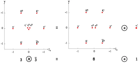
l = 0 states are the pseudoscalars 0−+ and the vectors 1−−. The orbital excitations l = 1 are the scalars 0++, the axial vectors 1++ and 1+−, and the tensors 2++. According to the SU(3) symmetry, the nine possible q ¯q combinations containing the light u, d, and s quarks are grouped into an octet and a singlet of light quark mesons: 3⊗3 = 8⊕1, as shown in Fig. 1.1 for the pseudoscalar mesons. The singlet with Y = 0 and I = 0 contains all the quarks on an equal
Figure 1.1: Pseudoscalar mesons arranged in SU(3) octet and singlet. footing. The normalized singlet state is
|1SU(3);|~I| =0i ≡ψ1=1/ √
1.2. Mesons mixing
symmetric in flavour, where n is the dimensionality of the representation. Of the two states at the centre of the octet, one belongs to an isospin triplet (isovector) and the other is an isospin singlet (isoscalar), both have I3=0. The quark wavefunction of the I3=0 triplet state is
|8SU(3);|~I| =1i ≡ψV =1/ √
2(u ¯u−d ¯d). (1.2)
Since the s and ¯s quarks are isospin singlets, they cannot couple to give an I=1 state. However, they can couple to give an I=0 state so that the I =0 state at the center of the octet is a linear combination of u ¯u, d ¯d and s ¯s. The properly normalized state, orthogonal to (1.1) and (1.2), is
|8SU(3);|~I| =0i ≡ψ8=1/ √
6(u ¯u+d ¯d−2s ¯s). (1.3) Pseudoscalar mesons have angular momentum J = 0: quark and antiquark are in the min-imum energy state, with relative angular momentum l = 0, and have opposite spin. The correspondence between pseudoscalar mesons and q ¯q states is: K+ = u ¯s, K0 = d ¯s, π− = ud,¯
K− = us, K¯ 0 = ds, π¯ + = u ¯d. The pseudoscalar mesons π0, η, η′, that have quantum numbers
Q = 0, I3 = 0, Y = 0, are represented as orthogonal combinations Auu ¯u+Add ¯d+Ass ¯s, with
normalized amplitudes|Au|2+ |Ad|2+ |As|2= 1.
1.2
Mesons mixing
The mass splitting in the multiplets show that although flavour SU(3) describes the hadron spectrum very well, it is not an exact symmetry. If it were, indeed, the states in a given mul-tiplet would be degenerate. In the pseudoscalar sector, assuming that the π0 meson has no strangeness component (mπ0 < ms) and is the (u ¯ud ¯d)/
√
2 state, SU(3)-breaking causes the physical η0and η′mesons to be mixtures of the SU(3) octet and singlet states:
η=η8cos θP−η1sin θP,
η′ =η8sin θP+η1cos θP, (1.4)
where η′ and η are the physical states, η1 and η8 are the singlet and octet state respectively
and θP is the mixing angle in the pseudoscalar nonet. The physical states η′ and η are
re-lated to the SU(3) singlet and octet states by a rotation of the angle θP. For small values of θP
the parametrization (1.4) implies that η′ is mainly a singlet state and η mainly an octet state. Assuming the mass matrix elements to be quadratic rather than linear (according to chiral per-turbation theory), H Ã η1 η8 ! = Ã M112 M182 M2 18 M882 ! Ã η1 η8 ! . (1.5)
After diagonalization of the mass matrix one derives [2]: tan2θP =
M882 −m2η m2η′−M288
with M2
88 = 1/3(m2K−m2π). Similar expressions exist for the vector and tensor meson nonets
in which there are φ−ω and f2′ − f2 mixing respectively. The sign of the mixing angle is
negative (positive) according to whether the mass of the mainly octet member is smaller than (greater than) that of the mainly singlet member. Important predictions about the dominant decay modes of the isoscalar states come from the observation that the 1−and 2+ nonets are almost “ideally mixed”. The singlet and octet wavefunctions for the isoscalar states are defined in (1.1) and (1.3), and the octet-singlet mixing is, for the general case, parametrized by
m8 =ψ8cos θ−ψ1sin θ ,
m1= ψ8sin θ+ψ1cos θ , (1.7)
where m1and m8are the physical, mainly singlet meson and the physical, mainly octet meson
respectively. If sinθ = 1/√3, where θ is the mixing angle, one has m1 ≈ u ¯u+d ¯d and m8 ≈ s ¯s.
In this case the nonet is said to be ideally mixed because the singlet state consists only of u ¯u
and d ¯d quarks and the octet state only of s ¯s quarks. Ideal mixing happens for θ≈35o, which is approximately the case for the 1−and 2+nonets but not for the pseudoscalar nonet. Therefore, for the members of these nonets, the mainly singlet states decay predominantly to pseudoscalar mesons consisting of u and d quarks (pions) and the mainly octet states to strange pseudoscalar mesons (kaons): BR(φ → K ¯K) ≈ 83%, BR(ω → π+π−π0) ≈ 89%, BR(f2′ → K ¯K) ≈ 89%,
BR(f2→ππ) ≈85%.
1.3
γγ coupling of mesons
The nonet mixing angles can be measured in γγ collisions. The γγ couplings of mesons can be expressed in terms of coupling constants gMγγ. For pseudoscalar and scalar resonances one
can define [4]: ΓPγγ= m 3 P 64πg 2 Pγγ, ΓSγγ = m 3 S 16πg 2 Sγγ. (1.8)
In the quark model mesons are represented as
|Mi =Σqcq|qqi. (1.9)
The coupling of two photons (with a given γγ helicity) to a quark-antiquark pair is proportional to the square of the quark charge:
hqq|γγi ∼e2qψq(0)(S wave) ,
1.3. γγ coupling of mesons
where ψq(0)is the radial quark wave function at the origin and ψ′q(0)is the first derivative of
ψq(0)at zero. If ψq(0)is independent of the quark flavour the γγ coupling constant of a meson
M can be related to the quark charge through (1.9) and (1.10):
gMγγ∼ hM|γγi ∼Σqcqe2q= he2qi. (1.11)
The coefficients cq are given by the SU(3) representations shown in (1.1)-(1.3). The effective
squared charges defined in (1.11) are
he2qiV = (e2d−e2u)/ √ 2=1/(3√2), he2qi8 = (e2u+e2d−2e2s)/ √ 6=1/(3√6), (1.12) he2qi1 = (e2u+e2d+e2s)/ √ 3=2/(3√3),
where the indices 8 and 1 denote the flavour octet and flavour singlet isoscalars, while the symbol V denotes the isovectors (e.g. π0, a2). Since the SU(3) symmetry is broken by the mass
of the s quark, the physical states are mixtures of the SU(3) singlet and octet states, as explained in the previous section. Therefore, neglecting any possible mass dependence, the ratios of the coupling constants depend only on the quark charges and on the mixing angle:
gπγγ : gηγγ : gη′γγ= ga2γγ : gf′γγ : gf γγ =
he2qiV : cos θhe2qi8−sin θheqi2 1: sin θhe2qi8+cos θhe2qi1 = √
3 : cos θ−2√2 sin θ : sin θ+2√2 cos θ . (1.13) A possible mass dependence for the coupling constant gMγγis strongly model dependent.
The first two-photon experiment proposed for e+e−storage rings was the measurement of the
π0 width [5]. The π0 → γγ decay played a fundamental role in the determination of the
number of color degrees of freedom of the quarks and therefore became a milestone for the development of the color gauge theory, “quantum chromodynamics” (QCD). The γγ width of the π0is connected to the γγ widths of the η and the η′mesons through the relations [6]:
Γη→γγ Γπ0→γγ = 1 3 m3η m3 π " fπcos θP fη8 − √ 8 fπsin θP fη1 #2 , (1.14) Γη′→γγ Γπ0→γγ = 1 3 m3η′ m3 π " fπsin θP fη8 − √ 8 fπcos θP fη1 #2 , (1.15)
where fπis the pion decay constant, fπ ≈93 MeV, θPis the pseudoscalar mixing angle, fη1and fη8 are the decay constants for the combinations η1 and η8. The ratio f8/ fπ ≈ 1.25 has been
calculated using chiral perturbation theory. Therefore the measurement of the partial γγ width Γ(X→γγ)is a crucial input for the determination of the pseudoscalar mixing angle.
1.4
Scalar mesons
Scalar mesons belong to the multiplet JP = 0+. They are grouped in a nonet, like the pseu-doscalar mesons, but the mass spectrum is inverted, as shown in Fig. 1.2. This inversion does not have any explanation within the usual description of mesons in terms of q ¯q couples. Moreover, the scalar mesons have positive parity, which is not possible in a q ¯q combination
Figure 1.2: Mass spectrum of the scalar mesons (left) and pseudoscalar mesons (right).
with angular momentum l = 0. One of the models used to describe the nature of the scalar mesons is the “tetraquark model”, that predicts the existence of four valence quarks: a couple of quarks (diquark) and a couple of antiquarks (antidiquark). This model explains the inverted mass spectrum. In Tab. 1.2 the quantum numbers of the light scalar mesons (with mass < 1
GeV) are shown. In contrast to the vector and tensor mesons, the identification of the scalar
I I3 S Y composition a+ 1 +1 0 0 [su][¯s ¯d] a0 1 0 0 0 √1 2([su][¯s ¯u] − [sd][¯s ¯d]) a− 1 -1 0 0 [sd][¯s ¯u] f0 0 0 0 0 12([su][¯s ¯u] + [sd]¯s ¯d) σ 0 0 0 0 [ud][u ¯¯d] K+ 1/2 +1/2 +1 +1 [ud][¯s ¯d] K0 1/2 -1/2 +1 +1 [ud][¯s ¯u] ¯ K0 1/2 +1/2 -1 -1 [us][d ¯¯u] K− 1/2 -1/2 -1 -1 [ds][d ¯¯u]
Table 1.2: Quantum numbers and scalar mesons composition in the diquark-antidiquark model.
mesons is a long-standing puzzle. Scalar resonances are difficult to resolve because some of them have large decay widths which cause a strong overlap between resonances and back-ground. Scalar mesons can be produced in πN scattering, p ¯p annihilation, J/ψ, B-, D- and
Chapter 2
Photon-photon interactions
2.1
Physics with two photons
Light by light scattering [4, 7, 8, 9, 10] is forbidden in classical electrodynamics because accord-ing to Maxwell’s classical linear equations electromagnetic waves cross each other without any disturbance. In quantum electrodynamics (QED), however, the situation is different. The un-certainty principle allows a photon of energy Eγto fluctuate into states of charged particle pairs
with mass mpair. The lifetime of this intermediate state, ∆t ≈ 2Eγ/m2pair, can be very large for
high values of Eγ, and photon-photon scattering becomes possible due to the interaction of
the intermediate particles. In other words, the photons create virtual pairs by quantum fluc-tuations of the vacuum. The simplest mechanism for elastic γγ scattering is given by the box diagram (Fig. 2.1). Very intense sources of photons are electron and positron storage rings,
Figure 2.1: Box diagram for elastic γγ scattering.
which were built to investigate the annihilation of electrons and positrons. In the lowest order of the electromagnetic coupling constant α, O(α2), this process can be seen as the annihilation of e+e−into a virtual time-like photon, which then materializes into a final state X of hadrons or leptons, as shown on the left side of Fig. 2.2. In the dominant diagram of the two-photon mechanism (right side of Fig. 2.2), instead, electrons and positrons of both incident beams emit virtual space-like photons that annihilate producing the final state X, which is some arbitrary final state allowed by conservation laws. In particular, hadronic states with JPC = 0±+; 2±+ are directly produced through the γγ → X subprocess. The cross section of the process is of
the order α4and is very small at low beam energies (up to several hundred MeV) if compared with the e+e−annihilation cross section. However, the two-photon cross section increases with
Figure 2.2: Feynman diagrams for e+e−annihilation (left) and γγ interactions (right). the beam energy E like(logE/me)2, while the e−e−annihilation cross section decreases at least like 1/E2. Therefore the two-photon process, despite of the order α4, already dominates over the annihilation process (of the order α2) for beam energies of a few GeV. The structure of the photon propagators in γγ reactions causes the photons to be radiated nearly on-mass-shell (al-most real photons) and at small angles (∼ me/E) relative to the beam axis. The momentum
transferred to the system X is therefore small. Most γγ events produce a low invariant mass final system, because of the typical bremsstrahlung spectrum of the emitted photons (∼1/Eγ).
The two-photon production of lepton pairs can be used to test quantum electrodynamics (QED) up to the order α4, while the production of hadronic final states gives the possibility of prob-ing hadron dynamics and studyprob-ing the couplprob-ing of the photons to quarks. In the regime of large four-momentum transfer q2 of the photons and high transverse momenta of the
pro-duced hadrons, the elementary nature of the photon is emphasized and the two photons have a pointlike coupling to a quark pair (high-pT jets, structure functions). The investigation of
the production of high transverse momentum particles, jets, and scattering of highly virtual photons, allows for tests of QCD. In the regime of low four momentum transfer q2 and low transferse momenta of the hadrons, the hadronic nature of the photon is emphasized, and al-most real photons are emitted. In the vector meson dominance (VMD) model [11], which works fairly well in most processes involving real or almost real photons, the photons turn into virtual vector mesons (e.g. ρ, ω, φ) which then interact strongly with hadrons (Fig. 2.3).
Figure 2.3: The dual nature of the photon: QED coupling (left) and and VMD coupling (right). The first theoretical papers related to two-photon physics at e+e− storage rings appeared in 1960. At the end of the 1960s and early 1970s the storage rings in Frascati, Novosibirsk, Or-say, Stanford and Hamburg became available. The first experimental results were obtained by ADONE in Frascati [12] and by VEPP-2 in Novosibirsk [13]. Since then, γγ interactions have
2.2. Kinematics and cross section of γγ reactions
been used to study the production of hadrons in almost all e+e− colliders in a variety of con-ditions in low- and high-q2 processes [10]. Both γγ∗ (one almost real photon and one virtual photon) and γγ (two almost real photons) reactions, exclusive and inclusive and for different regimes of photon-photon center of mass energy W, give crucial information on hadronic struc-ture. At low to medium W, the main goal of exclusive γγ studies is to extract the two-photon widths of meson resonances that couple to two photons. The measurement of the radiative width of pseudoscalar mesons Γ(X→γγ)is a crucial input for the determination of the pseu-doscalar mixing angle (see sections 1.2-1.3) and for testing the valence gluon content in the
η′ wavefunction [14]. On the other hand, a precise study of the form factors of the transition
γγ∗ → X, F(Q2
γ∗, 0), where one photon is off-shell and the other one is real, allows one to test
phenomenological models used for computing the light-by-light contribution to the(g−2)µ
prediction in the Standard Model [15] and the dynamics of the π0→e+e−transition [16].
2.2
Kinematics and cross section of γγ reactions
Two-photon scattering at e+e− storage rings can be observed through the reaction e+e− →
e+e−γ(∗)γ(∗)→e+e−X: an electron and a positron radiate photons, and these photons produce
the final system X with even C-parity. The kinematics of the reaction is completely determined by the four-momenta of the incoming and of the scattered electron and positron (see Fig. 2.4). The main goal is to find the amplitudes for the γγ → X process, both for virtual and almost
Figure 2.4: Kinematics of the two photon reaction e+e−→e+e−X.
real photons. The colliding photons with momenta q1 and q2 are space-like (q2 < 0) and may
have both a transverse (T) polarization and a longitudinal (L) polarization. The mass of the produced system is W2 = (q1+q2)2. The observed e+e− → e+e−X cross section is expressed
in terms of the γγ → X cross sections for the corresponding photons: σTT, σTL, σLT, σLL, e.g.
σTL is the cross section for the collision of a transverse photon q1 with a longitudinal photon q2. Moreover, the result has four additional interfering terms: τTT, τTL, τTTa , τTLa , where τTT
orthogonal (⊥) linear polarizations, and τa
TT is the difference between the cross sections for
scattering of transverse photons in states with total helicity 0 (σ0) and 2 (σ2):
τTT = σk−σ⊥; τTTa =σ0−σ2; σTT =1/2(σk+σ⊥) =1/2(σ0+σ2). (2.1)
The terms τTLand τTLa are connected with the interference terms of amplitudes for the transition
γγ → X where both transverse and longitudinal photons participate. All these quantities
depend on W2, q21and q22only. The differential cross section for the two-photon production has the form dσ(e+e−→e+e−X) = α 2q(q 1q2)2−q21q22 32π4E2q2 1q22 ×d 3p′ 1d3p′2 E′ 1E2′ × [4ρ++1 ρ2++σTT +2ρ++1 ρ002 σTL+2ρ001 ρ++2 σLT+ρ001 ρ002 σLL+2|ρ1+−ρ+−2 |τTTcos2 ˜φ −8|ρ+10ρ2+0|τTLcos2 ˜φ+AτTTa +BτTLa ]. (2.2)
The mixture of polarization states of the photon is given by a 3×3 density matrix with elements
ρµνi (i = 1, 2 for the two photons). The quantities ρab1,2are the elements of the density matrix of the virtual photons in the γγ helicity basis (a, b= ±1 for transverse photons, 0 for longitudinal photons), and can be expressed in terms of the momenta piand qiand the particle form factors.
The transformation between the two different bases (linear polarization basis and helicity basis) is derived in [9]. The term ˜φis the angle between the lepton scattering planes in the γγ center-of-mass system. Symmetry between photons requires σTL(W, q21, q22) =σLT(W, q22, q21), reducing
the number of independent functions to be determined. The coefficients of τTT and τTL both
vanish after the integration over ˜φ. The terms τTTa and τTLa can only be measured with polarized lepton beams, otherwise A = B = 0. All terms with an index L vanish if the corresponding photon is on-shell. Only σTT and τTT survive as both photons become real.
2.3
Approximations for the cross section formula
The complicated helicity structure of the cross section in equation (2.2) can in some cases be simplified [7, 8, 9]. Because of the photon propagators in γγ processes, the emitted photons are almost real, and one can make the approximation that only transverse photons contribute. The cross section 2.2 contains then only the term σTT (the term τTT vanishes after integrating over
˜ φ): dσ(e+e−→e+e−X) = α 2q(q 1q2)2−q21q22 32π4E2q2 1q22 ×4ρ++1 ρ++2 σTT× d 3p′ 1d3p′2 E1′E2′ . (2.3)
The e+e−→e+e−X cross section has been approximated by a product of the transverse photons
2.3. Approximations for the cross section formula
function” for transverse photons, LTT
γγ, the cross section can be rewritten as
d5σ(e+e− →e+e−X) dω1×dω2×dcosθ1×dcosθ2×dφ = d 5LTT γγ dω1×dω2×dcosθ1×dcosθ2×dφ × σTT, (2.4)
where ωi = Eγi/E. The differential luminosity function is
d5LTT γγ dω1×dω2×dcosθ1×dcosθ2×dφ = α 2E′ 1E2′ 16π3q2 1q22 ×4ρ++1 ρ2++√X , (2.5) where X= 1/4(W2−q2 1−q22)2−q21q22. The terms ρ ++
i contain in general the variables of both
photons. However, for q2i →0, q2i <<W2, it is possible to write the photon luminosity function
as a product of two fluxes. Since q2i <<W2, W2depends only on the energies of the photons: W2 = (q
1+q2)2 ≈4Eγ1Eγ2. After integrating over the angular distribution of the leptons, one
obtains the factorized luminosity function:
d2Lγγ dω1×dω2 = dNγ(ω1) dω1 × dNγ(ω2) dω2 . (2.6)
The photon spectra, integrated between q2
minand q2max<<W2, become
dNγ(ω) dω = α 2πω ½ [1+ (1−ω)2]lnq 2 max q2min − (1−ω) µ 1− q 2 min q2 max ¶¾ . (2.7)
Keeping only the leading term in (2.7) the photon spectrum is approximated by
dNγ(ω)/dω= (α/π)(1/ω)ln(E/me)[1+ (1−ω)2]. (2.8) The differential luminosity dLγγ/dz (where z = W/2E) can be obtained by integrating (2.6)
with the constraint ω1ω2=z2and with the approximation (2.8): dLγγ dz = µ 2α π ¶2µ ln E me ¶2 f(z) z , (2.9)
where the “Low function” f(z)is defined as
f(z) = (2+z2)2ln(1/z) − (1−z2)(3+z2). (2.10) For not too large values of z (z<0.8), this formula overestimates the exact luminosity function
by about 10% to 20%, but reproduces quite well the shape of the function. The factorization (2.6) is called “Equivalent Photon Approximation” (EPA) or “Weizs¨acker-Williams Approximation”. This approximation gives the exact cross section in the case where both scattered e+e− are detected within small forward angles. Fig. 2.5 shows the luminosity function multiplied by an integrated e+e− luminosity Lee = 1 fb−1, as a function of the γγ invariant mass for three
Figure 2.5: Differential γγ luminosity as a function of the center- of-mass energy. Accessible final states are also indicated.
2.4
Resonance production in γγ interactions
The total cross section for the production of a hadronic resonance R by two real photons is given by the (relativistic) Breit-Wigner formula
σ(γγ →R) =8π(2J+1) ΓΓγγ (W2−M2
R)2+Γ2M2R
, (2.11)
where J denotes the spin of the resonance, MR its mass, Γ and Γγγ its total and two-photon
decay width, and W the γγ center of mass energy. For a narrow resonance with J = 0 (e.g. pseudoscalar mesons) the cross section is
σ(γγ→R) =8π2Γγγ
MR
δ(W2−M2R). (2.12)
For almost real photons (Equivalent Photon Approximation) the cross section of the process
e+e− →e+e−R can be estimated from the expression:
σ(e+e−→e+e−R) = Z
dzdLγγ
dz σγγ→R(z). (2.13)
Implementing the cross section formula for a narrow resonance R, σ(γγ → R), in equation (2.13) one obtains the resulting cross section:
σ(e+e−→e+e−R) = 16α 2Γ γγ M3R µ ln E me ¶2· (z2+2)2ln1 z − (1−z 2)(3+z2) ¸ , (2.14)
2.5. Tagging of the photons
where the Low function has been used. This formula can be used to study the processes e+e− → e+e−π0, η, η′. Tab. 2.1 shows the cross section values for pseudoscalar mesons production in
γγinteractions for different values of√s.
R √s=1 GeV √s =1.02 GeV √s= 1.2 GeV √s=1.4 GeV
π0 266 271 317 364
η 43 45 66 90
η′ 3.3 4.9 20.0 39.7
Table 2.1: σe+e−→e+e−R[pb] calculated with the Equivalent Photon Approximation for different
values of√s.
2.5
Tagging of the photons
In experiments with two-photon interactions it is possible to “tag” the interacting photons by detecting the scattered leptons. There are three different kinematical conditions: both scattered leptons are detected (double-tag), only one scattered lepton is detected (single-tag), neither of the leptons is detected (no-tag). In principle the double-tag condition is the best one for measuring γγ processes because it gives complete information on the γγ system. However, most of the photons are emitted at small angles with respect to the beam axis, and the rate of events drops steeply when the leptons scatter away from the very forward direction. Tagging at very small angles is in most cases not easy because of background problems (small angle Bhabha scattering, beam-gas interaction). Furthermore, the energy loss of the scattered leptons is measured less accurately at higher energies, and the resolution of the γγ center of mass energy becomes worse. Most experimental results have been obtained with the single-tag or no-tag conditions. Single-tag is required when the background from one-photon annihilation events is not small or when one wants to determine the q2dependence of resonance couplings or of the total cross section (see section 2.6). Experimental experience has shown that if one wants to study exclusive final states with almost real photons, tagging is often not necessary. For the rejection of the background it is possible to take advantage of the fact that photons are mainly radiated along the beam direction, and the transverse momentum of the γγ system is small.
2.6
Form factors in meson-photon-photon transitions
The study of γγ interactions is useful to learn the properties of the strong interactions. Despite the probe and the target are both photons that carry electromagnetic force, they can produce a pair of quarks that interact strongly and are observed as hadrons, e.g. pseudoscalar mesons. However, the transition between a meson and two photons cannot be calculated from QCD directly, because at low energies the strong coupling constant αSis too large for a perturbative
including the effects of quarks and gluons, and at the end these effects are taken into account in an extra factor, known as “transition form-factor” (see Fig. 2.6). The form-factor connects three
Figure 2.6: General Pγ(∗)γ(∗)vertex described by a transition form factor, where P is a pseu-doscalar meson.
particles and therefore depends on three variables, the squared momenta q2i of the photons and the q2PSof the pseudoscalar. However, under the approximation that the quark mass is zero, the pseudoscalar becomes mass-less, q2
PS =0 (unlike the photons, which can be virtual). Therefore
F(q21, q22, q2PS) = F(q12, q22, 0) = F(q21, q22). The shape of the form-factor is not known exactly, but there exist some constraints on it [19]. Three of them come from QCD calculations:
• when the two photons are real, q2
i = 0, the transition can be seen as a point-like process
and the form-factor must fulfill the relation F(0, 0) =1;
• when both photons are are highly virtual and with equal value of q2, q2
1 =q22 =q2<<0,
the form factor is F(q2
1, q22) = −8(π fπ)2/Ncq2, where Nc is the number of colors in the
Standard Model, Nc =3, and fπis the pion decay constant;
• when one of the photons is real and the other one highly virtual, q2i =0 and q2j =q2<<0,
one must have F(0, q2) = −8(π fπ)2C/Ncq2, where C is a constant.
A fourth constraint derives from the fact that one believes that quark and gluon effects (not included in the pointlike description) correspond to intermediate states with other mesons, like the ρ meson. Therefore it should be possible to explain the shape of the form factor within the VMD model [20]. It is very difficult to find a form factor that satisfies all of these four constraints. The form factor
F(q21, q22) =1 (2.15)
satisfies only the first constraint. In this case there is no form factor, and the reaction is seen as pointlike. The form factor
F(q21, q22) = m 4 ρ (m2 ρ−q21)(m2ρ−q22) (2.16) satisfies the first and the fourth constraint, and with fπ = 92.4 MeV and mρ = 770 MeV it
satisfies the third constraint within the uncertainty on the constant parameter. The form factor
F(q21, q22) = m 2 ρ (m2 ρ−q21−q22) (2.17)
2.6. Form factors in meson-photon-photon transitions
satisfies the first three constraints but not the fourth one. The last form factor,
F(q21, q22) = m 4 ρ−4π 2F2 π NC (q 2 1+q22) (m2 ρ−q21)(m2ρ−q22) , (2.18)
satisfies constraint one, two and four.
The cross section for the process γγ→ R, where R is a narrow resonance, can be written as:
σγγ→R(q1, q2) =ΓR→γγ8π 2 MR
δ((q1+q2)2−M2R)|F(q21, q22)|2. (2.19)
If the photons are real the form factor dependence disappears. The transition form factors associated to the meson-photon-photon vertex can be accessed in the space-like region (q2<0)
by single-tag two photon experiments, when the momentum q2i of one photon is varied and the
q2j of the other photon is kept small (single-tag condition). Available data on|Fπ0(q2, 0)|and
|Fη(q2, 0)|for low|q2|values are presented in Figs. 2.7 and 2.8 [21]. Both processes π0 →γγ∗
and η→γγ∗can be described by the VMD model.
Figure 2.7: Single off-shell π0meson transition form factor in the low|q2|region from SND [22] and CMD-2 [23] data on the reaction e+e−→π0γand CELLO [24] data on the reaction e+e− →
Figure 2.8: Single off-shell η meson transition form factor from NA60 [25] data on η →γµ+µ−
decay; from SND [22] and CMD-2 [23] data on the reaction e+e− →ηγ, and from CELLO [24] data on the reaction e+e−→e+e−γ∗γ∗ →e+e−η.
2.7. Measurements of radiative widths of mesons
2.7
Measurements of radiative widths of mesons
In this section some measurements of partial widths ΓR→γγobtained with experiments at e+e−
storage rings are reported. With the MD-1 detector [17] at the VEPP-4 storage ring the following processes have been studied:
• e+e−→e+e−a2, with a2 →π+π−γγ,
• e+e−→e+e−η′, with η′ →π+π−γ, • e+e−→e+e−η, with η →γγ.
The center of mass energy is in the range [7.2-10.4] GeV, and the integrated luminosity is 20.8 pb−1. The results for the γγ widths are:
• Γ(a2→γγ) = (1.26±0.26±0.18)keV,
• Γ(η′ →γγ) = (4.6±1.1±0.6)keV, • Γ(η→γγ) = (0.51±0.12±0.05)keV.
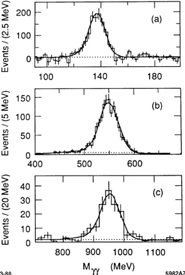
The Crystal Ball detector [6] at DORIS II (DESY) has been used to study the process e+e− → e+e−R, with R→ γγ, where R is a generic narrow resonance with mass between 100 and 3000 MeV. With an integrated luminosity of 114 pb−1and a center of mass energy between 9.4 and 10.6 GeV, three peaks are observed in the invariant γγ mass spectrum, corresponding to the pseudoscalar mesons π0, η and η′ (see Fig. 2.9). The results obtained for the γγ widths are:
• Γ(π0→γγ) = (7.7±0.5±0.5)keV, • Γ(η→γγ) = (0.514±0.017±0.035)keV, • Γ(η′ →γγ) = (4.7±0.5±0.5)keV.
The production of the η and η′ mesons in γγ interactions has also been observed with the detector ASP [18] at the PEP storage ring (SLAC), with a data sample of 108 pb−1and a center of mass energy √s = 29 GeV. The process studied is e+e− → e+e−R, with R → γγ. After a selection of 2287 η events and 547 η′ events, the following γγ partial widths are obtained:
• Γ(η→γγ) = (0.490±0.010±0.048)keV, • Γ(η′ →γγ) = (4.96±0.23±0.72)keV.
Figure 2.9: Distribution of the invariant γγ mass in the region of the π0mass (a), of the η mass
Chapter 3
The KLOE experiment at DAΦNE
The K LOng Experiment, KLOE, operates at the Frascati φ-factory DAΦNE. The main goal of the experiment is to measure direct CP violation in the neutral kaon system, analyzing K ¯K
couples produced in the φ meson decays. However, DAΦNE also produces a huge statistics of
ρ, ω, η, η′, f0, a0mesons. The KLOE physics program goes thus beyond the study of symmetry
violations in kaons, and covers many other topics, among which high precision studies on light hadron spectroscopy.
3.1
The collider DAΦNE
DAΦNE [26] (Double Annular Φ-factory for Nice Experiments) is an electron- positron collider designed to work at a center of mass energy corresponding to the mass of the φ resonance,
Mφ = (1019.456±0.020)MeV [1]. The accelerator complex consists of a LINAC, an
accumu-lator and a two-ring collider, as shown in Fig. 3.1. Electrons and positrons are accelerated up to 510 MeV in the LINAC and are then stored in the accumulator, where they are prepared for injection in the main rings. In order to reduce beam-beam interactions and to achieve high
Figure 3.1: Layout of the DAΦNE facility.
different rings and cross at the interaction point, IP, in two interaction regions with an angle in the horizontal plane (x-z) of 25 mrad, as shown in Fig. 3.2. This angle results in a small average
e+e−-momentum along the x-axis: < px,e+e− >≈ −12.7 MeV. Electrons and positrons circulate
ele pos
Figure 3.2: Layout of the DAΦNE main rings. The boxes indicate the two interaction regions. The KLOE detector is located in the lower one.
in the rings grouped in bunches. If L0is the single bunch luminosity, the total luminosity can
be expressed as:
L=n×L0=n×
νN+N−
4πσxσy, (3.1)
where n is the number of bunches, N+ and N− the number of positrons and electrons per bunch, ν the collision frequency, σx and σythe transverse (horizontal and vertical respectively)
dimensions of the bunch at the IP. The bunch dimensions are kept small at the IP by using a triplet of quadrupoles, which focus the beam in the vertical direction. The bunch sizes are
σx = 0.2 cm, σy = 20 µm, σz = 3 cm. The beams collide with a frequency up to 370 MHz,
corresponding to a minimum bunch crossing period of Tbunch =2.7 ns and a maximum number
of 120 bunches in each ring.
3.2
The KLOE detector
The KLOE detector was designed to collect the largest amount of neutral kaons from φ decays. The size of the apparatus is driven by the decay length of the KL, which at DAΦNE is about 340
cm. The detectable decay products of neutral kaons are pions, electrons, muons and photons, the latter coming mainly from neutral pion decays. The momentum spectra, limited by the kaons low energy, range between 50 and 300 MeV/c for charged particles and between 20 and 300 MeV/c for photons [27]. The detector has to be efficient for these energy ranges, minimiz-ing the losses due to geometrical acceptance. Fig. 3.3 shows a section of the detector. The main components are:
• a large, highly efficient drift chamber which measures trajectories and momenta of charged particles;
3.2. The KLOE detector S.C. COIL Barrel calorimeter DRIFT CHAMBER End Cap Cryostat Pole Piece YOKE 6 m 7 m
Figure 3.3: Vertical section of the KLOE detector.
• an electromagnetic calorimeter (barrel and endcaps) with excellent timing capabilities, to measure the energy deposits and the impact points of photons;
• a second electromagnetic calorimeter located in the narrow space between the drift cham-ber and the beam focusing quadrupoles, to improve acceptance and hermeticity;
• a superconducting coil which surrounds all the detectors and produces an axial magnetic field B =0.52 T.
The beam-pipe at the interaction point is made of a beryllium-aluminum alloy, 0.5 mm thick, to reduce multiple scattering, kaon regeneration, energy loss of particles and photon conversion, and encloses an interaction region made of a 10 cm radius sphere.
3.2.1 The drift chamber
The design of the KLOE drift chamber (DC) [28] was guided by the event topology of the KL
decays. Five main physics requirements have to be fulfilled:
• high and uniform reconstruction efficiency over a large volume;
• good momentum resolution (δpT/pT ≈ 0.4%) for low momentum tracks (50 < p < 300
MeV). The dominant contribution to the momentum resolution is multiple scattering:
δpT pT = 0.053 |B|Lβ s L X0, (3.2)
where pT is the transverse momentum in GeV, β is the velocity of the particle, L is the
track length in m, B is the magnetic field in T and X0is the radiation length;
• transparency to low energy photons (down to 20 MeV), and minimization of KL
regener-ation;
• a track resolution in the transverse plane σRΦ ≈200 µm, a vertex resolution σvtx≈1 mm,
and a z resolution σz ≈2 mm over the whole sensitive volume;
• fast trigger for neutral and charged particles.
The solution that meets the above requirements is a large cylindrical drift chamber, 3.3 m in length and 2 m in radius, around the IP. The uniform filling of the chamber has been achieved through a structure of drift cells almost square shaped, arranged in coaxial layers with alter-nating stereo angles which increase in magnitude with the radius from ± 60 to ± 150 mrad (Fig. 3.4). The stereo angle is defined as the angle between the wire and a line parallel to the
Figure 3.4: The KLOE drift chamber without the external wall.
z-axis passing through the point on the plate of the DC, where the wire is connected (Fig. 3.5). Uniformity of response is obtained with a ratio of field to sense wires of 3:1, which is a
satisfac-ε α z x y R p 0 R L
3.2. The KLOE detector
tory solution that ensures good electrostatic properties of the drift cell while still maintaining an acceptable track sampling frequency. Gold-plated tungsten wires are used as anodes (diam. = 25 µm). For the field wires, silver-plated aluminum wires have been chosen (diam. = 80 µm). There are 12 inner and 46 outer layers, the corresponding cell areas are (2×2) cm2 and (3×3)
cm2, respectively, for a total of 12582 single-sense-wire cells and 52140 wires. The gas used is a 90% helium, 10% isobutane mixture. The helium is the active component, its low atomic mass reduces multiple scattering and regeneration. The isobutane acts as quencher, absorbing the photons produced in recombination processes and avoiding the production of discharges in the DC. The mixture has a radiation length X0≈1300 m. Taking into account also the presence
of the wires, the average radiation length in the whole DC volume is X0 ≈ 900 m. The
sig-nals coming from sense wire are amplified, discriminated and transmitted to read-out system: ADC for dE/dx measurement and TDC for time meausurement. Samples of Bhabha-scattering events allow evaluation of the momentum resolution for 510 MeV e±(Fig. 3.6), as well as the beam energy at the IP, and the position and the shape of the luminous region. In the interval
momentum resolution (MeV/c)
polar angle (degrees)
Figure 3.6: Momentum resolution for Bhabha tracks as a function of the polar angle. 50◦ <θ <130◦the momentum resolution is σp≈1.3 MeV, σp/p =2.5×10⁻³.
3.2.2 The electromagnetic calorimeter
The KLOE electromagnetic calorimeter (EMC) [29] was designed to fulfill four main require-ments:
• good time resolution (≈100 ps) and good spatial determination of the photon conversion point (≈1 cm);
• hermeticity (98% of the solid angle), good energy resolution (≈5%/√E [GeV]) and high
efficiency over the range 20-300 MeV;
• fast first level trigger.
The above considerations have led to the choice of a lead-scintillating fiber sampling calorime-ter. Scintillating fibers offer many advantages, in particular they provide good light transmis-sion over the required distances, up to about 4.3 m. It is easy to adapt the calorimeter shape (Fig. 3.7) to geometrical requirements, obtaining good hermeticity. The cylindrical barrel
con-Figure 3.7: The KLOE electromagnetic calorimeter.
sists of 24 modules 4.3 m long, 23 cm thick and trapezoidal in cross-section, with fibers running parallel to the beam line. Each of the two endcaps consists of 32 vertical C-shaped modules 0.7 to 3.9 m long and 23 cm thick, with fibers running perpendicular to the beam line. The whole structure has a 98% solid angle coverage. All modules are stacks of 0.55 mm thick lead foils (passive material) alternating with layers of 1 mm diameter scintillating fibers (active material) (Fig. 3.8). The average density is 5 g/cm3, the radiation length is about 1.5 cm and the
over-Figure 3.8: Schematic view of the fiber-lead structure of the electromagnetic calorimeter for a barrel module.
all thickness of the calorimeter is about 15 radiation lengths. Light is collected at both ends of the fibers through light pipes, which match almost square portions of the module to 4880
3.2. The KLOE detector
photo-tubes (PMs). The read-out subdivides the calorimeter into five planes in depth, each 4.4 cm thick. In the transverse direction each plane is subdivided into cells 4.4 cm wide. The resulting read-out granularity is about 4.4×4.4 cm2. Signals from the PMs are split and sent to ADC’s for energy measurements and trigger, and to the TDC’s for time measurements. The time difference of the signal at both ends allows to reconstruct the coordinate along the fiber with a resolution σk ≈1.4 cm/√E [GeV]. The resolution in the orthogonal direction is σ⊥≈1.3 cm. Energy resolution and linearity have been measured using photons from radiative Bhabha events. Event reconstruction from tracking informations determines the photon direction and energy, Eγ, with good accuracy. The photon energy is then compared with the measured cluster
energy Eclu. The resolution σE/Eγ and the deviation from linearity(Eγ−Eclu)/Eγare shown
in Fig. 3.9 as a function of the photon energy. Linearity is better than 1% for Eγ > 75 MeV.
Figure 3.9: Top: linearity of the calorimeter energy response as a function of the photon energy. Bottom: energy resolution of the calorimeter as a function of the photon energy.
By fitting the energy resolution with a function a/√E [GeV]+b, one obtains a stochastic term a=5.7% and a negligible constant term, showing that the resolution is dominated by sampling fluctuations: σE Eγ = p 0.057 Eγ[GeV] . (3.3)
The time resolution has been obtained from the analysis of Bhabha events and radiative φ decays, and is shown in Fig. 3.10 as a function of the energy of the photon:
σt= p 57 ps
Eγ [GeV]⊕
where the sampling fluctuation term is in agreement with test beam data. The second term is a constant to be added in quadrature and is given by two contributions: the intrinsic time spread due to the finite length of the luminous point in the beam direction, and the resolution of the synchronization with the DAΦNE radiofrequency.
Figure 3.10: Time resolution of the calorimeter as a function of the photon energy.
3.2.3 The quadrupole calorimeters
The quadrupole tile calorimeters of KLOE (QCAL) [30] are two compact detectors, made of lead plates and scintillator tiles, that surround the focusing quadrupoles (Fig. 3.11). Their aim is to complete the hermeticity of the KLOE calorimeter for photons coming from the KL→ π0π0π0
decays. Each sector contains 16 absorber plates made of 1.9 mm thick lead, alternating with
Figure 3.11: The KLOE QCAL.
16 scintillator layers 1 mm thick. The scintillator layers are divided into three equal tiles. In the cylindrical section the tyles have rectangular shape, while in the conical section the shape is trapezoidal. In each layer, four 190 cm long wavelength shifting (WLS) fibers run along the sides of the tiles. Light is collected by PMs. The overall radial thickness is 5.5 X0.
3.2. The KLOE detector
3.2.4 The trigger system
The KLOE trigger system [31] was designed to: • produce a trigger signal for all φ decays; • recognize Bhabha and cosmic-ray events; • reject machine background.
The trigger is based on local energy deposit in the calorimeter and multiplicity information from the DC. It is composed of two levels in order to both produce an early trigger with good timing to start the acquisition operations and to use as much information as possible from the DC. After the arrival of a first level trigger, additional information is collected from the DC, which is used, together with the calorimetric information, to confirm the trigger and start the data acquisition system.
The EMC trigger
For trigger purposes the fine granularity of the calorimeter is not needed, therefore adjacent calorimeter columns are grouped together to form a “trigger sector” and their signals are summed. In order to guarantee that each “particle” is fully contained in at least one sum, the calorimeter signals form a set of totally overlapping sectors: “normal” and “overlap”. In the barrel, each trigger sector is made of 5 cells×6 columns, being the columns of each series placed on top of the other by half sector width (see Fig. 3.12). Since the particle multiplicity is
Figure 3.12: Trigger sectors in the barrel.
higher in the forward region, mostly for background events, the geometry of the end caps is more complex: they are segmented in groups of four columns in the zone close to the beam axis and of five/six columns elsewhere. The outer layer of the entire calorimeter is used as a cos-mic ray detector. The calorimeter triggers on local energy deposits larger than a programmable threshold. Two thresholds are used, one for the barrel (≈ 50 MeV) and one for the endcaps (≈ 150 MeV). In practice it is not easy to apply a threshold which corresponds to a constant energy deposit, because the signal amplitude depends on the position along the fibers of the
incident particle. This is due to the attenuation of the scintillator light in the optical fibers. In order to reduce the effect, the analog signals from both sides (A and B) of each calorimeter sec-tor are compared to two thresholds (Tlow, Thigh). The threshold settings and comparator output
are shown in Fig. 3.13. This scheme allows to apply a large variety of effective thresholds.
Figure 3.13: Effective trigger threshold as a function of the z-coordinate (along the fiber) of the incident particle.
The DC trigger
DC information can be used to produce a trigger for the π±,∓and π±,00channels, for which the
calorimeter trigger is less efficient. The DC trigger is based on the multiplicity of hit wires, i.e. on the sum of all signals from the 12582 DC sense wires. The sense wire signals, after preampli-fication, are brought to the ADS (Amplifier/Discriminator/Shaper) boards. On the ADS, each signal is discriminated, buffered, and split into two different paths. The first path is directed to the DC readout front-end; the second path is used for the trigger. In the trigger path, signals are formed with a width of 250 ns. The signals coming from the DC wires are organized in nine concentric ring sections called “superlayers”, which represent the multiplicity of hit wires in eight, six or four (from the innermost to the outermost) contiguous planes. The superlayers are defined in order to reduce the effect of low-momentum electrons spiralling inside the DC volume, which produce a large number of hit wires in the inner region of the detector.
The two-level trigger logic
The KLOE trigger is composed of two levels. The first level trigger (T1) is activated if there are two calorimeter fired sectors with barrel-barrel, barrel-endcap or endcap- endcap (not the same endcap) topology OR 15 DC hits within 250 ns. The T1 trigger sets a≈2 µs long acknowledge
3.3. Data reconstruction
signal, which vetoes other T1 triggers and allows signals formation from the DC cells. The second level trigger (T2) validates the T1 trigger and starts the data acquisition. Events with two fired sectors in the external planes of the calorimeter (see Fig. 3.12) with barrel-barrel or barrel-endcap topology are passed to a third level hardware algorithm, based on DC hits, which recognizes cosmic-ray events and rejects them.
3.2.5 Data acquisition
The KLOE data acquisition (DAQ) [32] has been designed to cope with a rate of 104 events
per second, due to φ decays, downscaled Bhabha events, non vetoed cosmic rays and DAΦNE machine background. An average event size of 5 kbytes is estimated, corresponding to a total bandwidth requirement of 50 Mbytes/s. The DAQ readout system involves some 23000 chan-nels of front end electronics (FEE) from EMC, DC and trigger system. For each event, relevant data coming from the whole FEE system have to be concentrated in a single CPU where a dedi-cated process builds the complete event. A three level scheme has been implemented. The first level reads data from single FEE crates. The second level combines information from different crates. The last level, responsible for final event building, relies on standard network media and protocols (TCP/IP).
3.3
Data reconstruction
Data reconstruction starts immediately after the completion of the calibration jobs. The recon-struction program, DATAREC [33], provides additional data-quality and monitoring informa-tion, and consists of several modules, among which EMC reconstrucinforma-tion, DC reconstrucinforma-tion, and track-to-cluster association.
3.3.1 Cluster reconstruction
The calorimeter is segmented into 2440 cells, which are read out by PMs at both ends (A, B). This segmentation provides the determination of the position of energy deposits in r−φfor the barrel and in x−z for the endcaps. Both charges QA,BADC and times tA,BTDC are recorded. For each cell, the particle arrival time t and its coordinate s along the fiber direction (the zero being taken at the fiber center) are obtained using the times at the two ends as
t(ns) = 1 2(t A+tB −t0A−t0B) − L 2v, (3.5) s(cm) = v 2(t A −tB−t0A+t0B), (3.6)
with tA,B = cA,B×tA,BTDC, where cA,B are the TDC calibration constants, t0A,B are the overall time offsets, L and v are the cell length and the light velocity in the fibers, respectively. The energy
![Figure 2.8: Single off-shell η meson transition form factor from NA60 [25] data on η → γµ + µ −](https://thumb-eu.123doks.com/thumbv2/123dokorg/2837743.4926/24.918.219.634.438.727/figure-single-shell-meson-transition-form-factor-data.webp)