v
I hereby declare that except where specific reference is made to the work of others, the contents of this dissertation are original and have not been submitted in whole or in part for consideration for any other degree or qualification in this, or any other University. This dissertation is the result of my own work and includes nothing which is the outcome of work done in collaboration, except where specifically indicated in the text.
Dott. Giuseppe Brunetti 2017
vii
And I would like to acknowledge all the people that shared with me this path. Everyone gave me something unique.
ix
The increasing frequency of flooding events in urban catchments related to an increase in impervious surfaces highlights the inadequacy of traditional urban drainage systems. Low-impact developments (LIDs) techniques have proven to be valuable alternatives for stormwater management and hydrological restoration, by reducing stormwater runoff and increasing the infiltration and evapotranspiration capacity of urban areas. However, the lack of diffusion of adequate modelling tools represents a barrier in designing and constructing such systems. Mechanistic models are reliable and accurate tools for analysis of the hydrologic behaviour of LIDs, yet only a few studies provide a comprehensive numerical analysis of the hydrological processes involved and test their model predictions against field-scale data. Moreover, their widespread use among urban hydrologists suffers from some limitations, namely: complexity,
model calibration and computational cost. This suggest that more research is needed to address
these issues and examine the applicability of this kind of models. Thus, the main aim of this thesis was to investigate the benefits and the limitations in the use of mechanistic modelling for LIDs analysis. In this view, the mechanistic modelling approach has been used to simulate the hydraulic/hydrologic behaviour of three different LIDs installed at the University of Calabria: an extensive green roof, a permeable pavement and a stormwater filter. Each case study was used to examine a particular modelling aspect. The morphological and hydrological complexity of the green roof required the use of a three-dimensional mechanistic model, which was validated against experimental data with satisfactory results. The measured soil hydraulic properties of the soil substrate highlighted important characteristics, accounted in the simulation. The validated model was used to carry out a hydrological analysis of the green roof and its hydrological performance during the entire simulated period as well as during single precipitation events. Conversely, a one-dimensional mechanistic model was used to simulate the hydraulic behaviour of a permeable pavement, whose parameters were calibrated against experimental data. A Global Sensitivity Analysis (GSA) followed by a Monte Carlo filtering highlighted the influence of the wear layer on the hydraulic behaviour of the pavement and identified the ranges of parameters generating behavioural solutions in the optimization
x
good results. Finally, to address the issue of computational cost, the surrogate-based modelling technique has been applied to calibrate a two-dimensional mechanistic model used to simulate the hydraulic behaviour of a stormwater filter. The kriging technique was utilized to approximate the deterministic response of the mechanistic model. The validated kriging model was first used to carry out a Global Sensitivity Analysis of the unknown soil hydraulic parameters of the filter layer. Next, the Particle Swarm Optimization algorithm was used to estimate their values. Finally, the calibrated model was validated against an independent set of measured outflows with optimal results. Results of the present thesis confirmed the reliability of mechanistic models for LIDs analysis, and gave a new contribution towards a much broader diffusion of such modelling tools.
xi
Contents ... xi
List of Figures ... xiii
List of Tables ... xvii
Chapter 1 Introduction ... 19
1.1 Urban Drainage Systems: issues and new challenges ... 19
1.2 Sustainable Stormwater Management ... 21
1.2.1 Modelling tools for LIDs analysis ... 23
1.3 Objectives and aim ... 25
Chapter 2 A comprehensive analysis of the variably-saturated hydraulic behaviour of a green roof in a Mediterranean climate ... 29
2.1 Introduction ... 29
2.2 Materials and Methods ... 33
2.2.1 Green Roof and Site Description ... 33
2.2.2 Soil Hydraulic Properties ... 38
2.2.3 Modeling Theory ... 42
2.2.4 Statistical Evaluation ... 49
2.3 Results and Discussion ... 50
2.3.1 Soil Hydraulic Properties ... 50
2.3.2 Model Validation ... 54
2.3.3 Hydrological Analysis of the Green Roof ... 58
2.3.4 Hydrological Performance during Precipitation Events ... 62
2.4 Conclusions ... 65
Chapter 3 A comprehensive numerical analysis of the hydraulic behavior of a permeable pavement 69 3.1 Introduction ... 69
3.2 Materials and Methods ... 74
3.2.1 Site Description ... 74
3.2.2 Theory ... 78
3.3 Results and Discussion ... 92
xii
3.3.5 Particle Swarm Optimization ... 102
3.3.6 Confidence Regions ... 107
3.3.7 Model Validation ... 108
3.4 Conclusions ... 112
Chapter 4 On the use of surrogate-based modeling for the numerical analysis of Low Impact Development techniques ... 115
4.1 Introduction ... 115
4.2 Materials and Methods ... 119
4.2.1 Stormwater Filter and Site Description... 119
4.2.2 Evaporation Method and Parameter Estimation ... 124
4.2.3 Modeling Theory ... 125
4.2.4 Surrogate Based Model ... 130
4.2.5 Global Sensitivity Analysis (GSA) ... 135
4.2.6 Particle Swarm Optimization ... 137
4.2.7 Objective Function ... 139
4.3 Results and Discussion ... 139
4.3.1 Evaporation Method... 139
4.3.2 Kriging Approximation of the Response Surface ... 141
4.3.3 Global Sensitivity Analysis... 143
4.3.4 Kriging-Based Optimization ... 145
4.3.5 Model Validation ... 152
4.4 Conclusions and Summary ... 154
Chapter 5 Conclusions and future directions ... 157
5.1 Future directions ... 160
xiii
Figure 1.1 A schematic of the current stormwater management ... 20 Figure 1.2 A schematic of a sustainable stormwater management ... 22 Figure 2.1 A typical cross-section of the GR. ... 34 Figure 2.2 A schematic of the green roof, showing both vegetated (grey) and non-vegetated (white) areas. Irrigation drippers are indicated by a letter D. ... 35 Figure 2.3 Measured precipitation (black), irrigation (top graph), and subsurface (gray) fluxes for a selected time period. ... 37 Figure 2.4 Details of the drainage layer, where d is the thickness of the open space between drainage holes, and the geotextile supporting the GR substrate. ... 45 Figure 2.5 Spatial distribution of considered boundary conditions. ... 46 Figure 2.6 Measured and modeled values of the retention curve (log10 (h)) (left) and the
hydraulic conductivity functions K(log10 (h)) (center) and K( ) (right). The measured values
are scatter points, the full and dashed lines are the fitted bimodal and unimodal functions, respectively. ... 51 Figure 2.7 A comparison between measured and simulated outflows versus time and against each other (in the insert). The full and dashed lines in the insert are bisector and linear
regression lines, respectively. ... 55 Figure 2.8 A lag plot of the residuals between measure and simulated outflows. Results are for the HYDRUS model with the unimodal (left) and bimodal (right) functions of soil
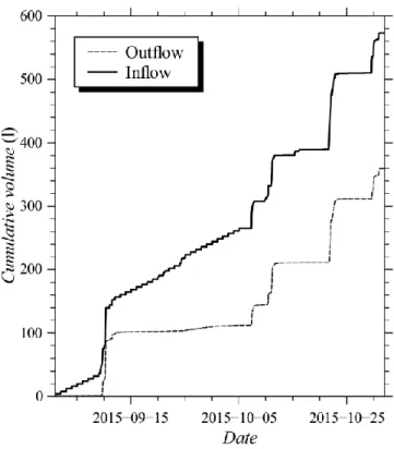
hydraulic properties. ... 57 Figure 2.9 A comparison between cumulative inflow and outflow from the GR, simulated by HYDRUS-3D. ... 59 Figure 2.10 Simulated actual root water uptake (top) and evaporation (bottom) from
vegetated areas of the green roof. ... 60 Figure 2.11 Pressure heads at the bottom of the vegetated (black) and non-vegetated (red) sections of the GR simulated by HYDRUS-3D. The yellow rectangular area in the top figure is expanded in the bottom figure. The dashed line represents a seepage condition. ... 61 Figure 2.12 Precipitation (dark area), modeled (grey area) and measured (red line) outflow for four selected rainfall events in the analysis of the hydrological performance of the GR during single precipitation events. ... 63
xiv
Figure 3.3 Scatter plots for pair relations a1-NSE (left) and n1-NSE (right) for Scenario I. The
red line is a regression line. ... 94 Figure 3.4 Bivariate KDE plots (below diagonal), univariate KDE plots (diagonal), and correlation plots (above diagonal) for Scenario I. ... 96 Figure 3.5 The average total index, ST, for different layers for both scenarios. ... 99
Figure 3.6 Scatter plots for pair relations a1-NSE (left) and n1-NSE (right) for Scenario II. The
red line is a regression line. ... 100 Figure 3.7 Bivariate KDE plots (below diagonal), univariate KDE plots (diagonal), and correlation plots (above diagonal) for Scenario II. ... 101 Figure 3.8 Comparison between the modeled and measured hydrographs for Scenarios I (top) and II (bottom) for the optimization process. ... 104 Figure 3.9 Comparison between the modeled and measured hydrograph for the two scenarios for the validation period. ... 109 Figure 3.10 Comparison between the modeled and measured outflows for the two scenarios for the validation period. ... 111 Figure 4.1 A schematic of the experimental site (top) and a typical cross-section (bottom) of the stormwater filter. ... 120 Figure 4.2 Precipitation (black line) and subsurface flow (grey line) for the optimization (top) and validation (bottom) periods, respectively. ... 123 Figure 4.3 The spatial distribution of applied boundary conditions. ... 129 Figure 4.4 Measured values and modeled functions of soil water retention, (log10(|h|)) (left)
and the unsaturated hydraulic conductivity, K(log10(|h|)) (center) and K( ) (right). Symbols
represent the measured values, and full lines the fitted VGM functions. ... 140 Figure 4.5 Comparison between the HYDRUS-2D and kriging-predicted values of the NSE for the validation sample. The initial (grey diamonds) and infilled (red circles) kriging models are compared. A bisector (a black line) and regression lines for the initial (a dashed grey line) and infilled (a dashed red line) kriging models are reported. ... 142 Figure 4.6 A comparison between measured and simulated outflows versus time and against each other (in the insert) for the calibration period. The full and dashed lines in the insert are a bisector and linear regression line, respectively. ... 147 Figure 4.7 The - Ks response surface obtained using a regular grid of 40,000 points. The red
lines indicate the cross sections reported in Figure 4.8. ... 149 Figure 4.8 Horizontal [Ks = 90 cm/min] (top), and vertical [= 0.001 1/cm] (bottom)
response surface cross-sections. The yellow rectangular areas for both plots are expanded on the right. ... 151
xvii
Table 2.1 Feddes’ parameters for the water stress response function used in numerical
simulations. ... 43
Table 2.2 Fluxes considered in different types of boundary conditions. ... 47
Table 2.3 Estimated soil hydraulic parameters and their confidence intervals (CIs) for the unimodal and bimodal hydraulic functions... 52
Table 3.1 Conceptual models representing water flow in the permeable pavement. ... 78
Table 3.2 Number of parameters and HYDRUS-1D runs for both scenarios. ... 86
Table 3.3 Ranges of parameters used in the GSA for both scenarios. ... 87
Table 3.4 Parameters used in the PSO optimization. ... 91
Table 3.5 First-order (S1) and total (ST) effect indices (in decreasing order) with their bootstrap confidence intervals (BCI) for parameters of Scenario I. ... 92
Table 3.6 First-order (S1) and total (ST) effect indices (in decreasing order) with their bootstrap confidence intervals (BCI) for parameter of Scenario II. ... 98
Table 3.7 Reduced ranges of optimized parameters for the optimization process. ... 103
Table 3.8 Optimized soil hydraulic parameters for both scenarios. ... 105
Table 3.9 Confidence intervals (CI) for optimized parameters for both scenarios. ... 107
Table 4.1 Ranges of investigated parameters for the surrogate-based analysis. ... 127
Table 4.2 Parameters used in the PSO optimization. ... 138
Table 4.3 Estimated soil hydraulic parameters and their confidence intervals for the soil substrate ... 141
Table 4.4 The first-order (S1) and total (ST) effect indices (in a decreasing order) with their bootstrap confidence intervals (BCI) for the soil hydraulic parameters. ... 144
Table 4.5 VGM parameters for the filter layer. The shape parameter and the saturated hydraulic conductivity Ks were estimated using the PSO algorithm. ... 146
Table 4.6 VGM parameters for the filter layer. The saturated water content θs, the shape parameters and n, and the saturated hydraulic conductivity Ks were estimated using the PSO algorithm. ... 152
19
Chapter 1 Introduction
“Sustainability” is not only a word, but a concept that is permeating our life in the last few decades. A concept that represents an abrupt and necessary change in our way of living; a change that is needed in order to not compromise the lives of the new generations:
« Development that meets the needs of the present without compromising the ability of
the future generations to meet their own needs».
This is the basic definition of sustainable development proposed at the World’s first Earth Summit in Rio de Janeiro in 1992. Before that date, the concept of sustainability was something rather marginal in the society, focused on the economic growth and industrial development after the tragedies of the second World War. The exponential demographic growth, the technological progress and the wild globalization pushed the society towards a new model, where individual needs are multiplied. To deal with this change, Earth’s resources were exploited at an unsustainable rate, disregarding the negative impacts on the environment. Air, soil and water pollution became the most important threats to the global health, with the appearance of new contaminants. The sustainability concept emerged as the unique viable approach to counterbalance and mitigate the negative impacts of the current development model.
1.1 Urban Drainage Systems: issues and new challenges
Progressing urbanization of undeveloped land leads to an increasing amount of impervious surfaces at the expense of natural areas. Leopold (1968), while describing the effects of urbanization on the hydrological cycle, identified such major effects as reduced
20
recharge. Traditional stormwater management design focused on collecting stormwater in piped networks and transporting it off-site as quickly as possible. Increases in the incidence of flooding and combined sewer overflows (CSOs) in urban areas demonstrate that the traditional approach is inadequate for managing stormwater. Traditional urban drainage systems are unable to cope with a constant increase of surface runoff due to structural limitations. Drainage systems, especially in European cities, consist of facilities built in different epochs, and designed to manage considerably lower runoff volumes. In such circumstances, it is quite usual to have in the same cities flooded and non-flooded districts, depending on the structure of the drainage system.
21
In a context where the resiliency of urban areas under climate change becomes crucial, the inadequacy of traditional urban drainage systems can pose serious problems. Urbanized landscapes are one of the most sensitive systems to hydrological extremes, fluctuations and changes. The change of precipitation regime, which is likely to occur in the immediate future, will increase the frequency of extreme precipitation events (Lenderink and van Meijgaard, 2008), known to be correlated with flash floods in urban areas. In such circumstances, it is necessary to treat the stormwater management as an urgent problem and find sustainable solutions able to cope with today’s and upcoming problems.
1.2 Sustainable Stormwater Management
As mentioned above, the combined effects of increased imperviousness and climate change is highlighting the inadequacy of traditional drainage systems in stormwater management. A theoretical alternative would be to replace existing piped networks with larger ones able to manage an increased surface runoff, but this poses economic and practical problems. Thus, it is necessary to shift the target to the reasons of runoff increase, namely the surface’s imperviousness, main cause of the alteration of the urban hydrological cycle. In this view, the sustainable stormwater management aims to preserve and restore natural features, minimize the imperviousness of urban catchments, and increase their infiltration and evapotranspiration capacities.
The so-called “Sponge cities” focus on mimicking the hydrology that existed prior to the development through the use of micro-controls distributed throughout a developed site. These micro-controls are located near the source where runoff is generated and help deliver it back to its natural pathway (through permeable materials into the ground, or through evaporation into the air). Micro-controls can include stormwater filters, green roofs, wetlands, permeable pavements and other measures that reduce both runoff volume and speed. Rain can also be harvested in cisterns for landscape irrigation and other beneficial uses. Such practices are
22 (GI).
Figure 1.2 A schematic of a sustainable stormwater management
Low-impact developments are able to reduce runoff volumes and pollutant loads and increase evapotranspiration. Green roofs were able to significantly reduce peak rates of stormwater runoff (Getter et al., 2007) and retain rainfall volumes with retention efficiencies ranging from 40 to 80% (Bengtsson et al., 2004). Bioretention cells were shown to reduce average peak flows by at least 45% during a series of rainfall events in Maryland and North Carolina (Davis, 2008). Permeable pavements offered great advantages in terms of runoff reduction (Carbone et al., 2014; Collins et al., 2008), water retention, and water quality improvement (Brattebo and Booth, 2003).
23
1.2.1 Modelling tools for LIDs analysis
In spite of the large and well-known benefits of green roofs and other LID techniques, the transition to sustainable urban drainage systems is very slow. One of the key limiting factors in the widespread adoption of such systems is the lack of adequate analytical and modelling tools (Elliot and Trowsdale, 2007) able to simulate all the physical processes involved. Several models have been proposed in the literature; most of them focused on simulating the hydraulic/hydrologic behaviour of the system.
Empirical models are models where the structure is determined by the observed relationship among experimental data. These models can be used to develop relationship for forecasting and describing trends, which are not necessarily mechanistically relevant. Typical examples of empirical models for LIDs analysis include relationships between the rain depth and the subsurface runoff coefficient, or between the antecedent dry periods and the surface runoff coefficient. The main drawback of this kind of models is the lack of generality. The accuracy of the empirical relation is strongly dependent on the size and characteristics of the sample used for the statistical analysis. For example, a relationship between the retention efficiency of a green roof in a continental climate, and the antecedent dry period will lead to inaccurate results if applied to a green roof in a mediterranean climate. Only by increasing the size and the variance of the sample, it would be possible to increase the robustness of the empirical model. However, even if the sample is statistically representative and significant, the uncertainty associated with the developed relationship could lead to biased conclusions.
An alternative is represented by conceptual models. A conceptual model is a descriptive representation of a system that incorporates the modeler’s understanding of the relevant physical processes involved. In this type of modelling, the different components of the system are described using conceptual entities. For example, the hydraulic behaviour of a porous media is described using a reservoir with a sharp-crested weir, whose height represents the field capacity, and whose discharge rate represents its hydraulic conductivity. Conceptual models have been used extensively in the literature for the numerical analysis of LIDs, in particular for green roofs. Kasmin et al. (2010) developed a simple conceptual model of the hydrological
24
precipitation events and the output was runoff. The water content in the green roof at any given time was between field capacity and the residual water content. Evapotranspiration was estimated using an empirical relationship accounting for the actual water contents, the storm event’s characteristics, and the antecedent dry weather period. During a precipitation event, the porous medium absorbed moisture until field capacity was reached. The addition of further moisture produced subsurface flow. Stovin et al. (2013) used a conceptual model to simulate the hydraulic behaviour of a green roof. In that model, the actual evapotranspiration is function of the potential evapotranspiration and substrate moisture content, and the retention capacity is conceptualized as a reservoir. While being quite fast and intuitive, conceptual models suffer from several limitations. Conceptualization of the physical processes involved often leads to simplification of the system and a reduction in numerical parameters. While in a physical model each parameter has its own meaning, in conceptual models, lumped parameters often incorporate different components of the described process. These lumped parameters are case sensitive and need to be calibrated against experimental data, implying a lack of generality of the model itself. These drawbacks could represent a barrier to the use of modeling tools among practitioners who need reliable and generally applicable models.
Conceptual models represent a middle ground between empirical and mechanistic models. While empirical models are based on direct observation, measurement and extensive data records, mechanistic models are based on the mathematical description of physical, chemical, and biological processes involved. One of the main advantage of mechanistic approach is that each component has a clear physical meaning, and each parameter can be measured independently. In spite of being accurate and general, mechanistic models are not widely for the numerical analysis of LIDs. This is mainly due to some drawbacks, which are typical in mechanistic modeling:
Complexity: in the mechanistic approach, each process is analysed separately
25
familiar with all the processes involved (i.e, infiltration, evaporation, transpiration, preferential flows, solute transport, heat transport, etc); Model calibration: The calibration of mechanistic models can be quite
challenging, and usually involves the optimization of several parameters. This requires the use of complex optimization algorithm and a careful
quantification of the uncertainty associated with each estimated parameter; Computational cost: Mechanistic models usually require the numerical
resolution of nonlinear partial differential equations. Depending on the type of problem, the computational cost associated with a single model execution can be significantly high, especially if several physical processes are modelled simultaneously. This cost increases exponentially if the modelling framework includes the calibration of several parameters, making impractical the use of the model itself.
1.3 Objectives and aim
The main aim of the present thesis is to investigate the use of mechanistic modelling for the numerical analysis of LIDs. In particular, the present study focuses on the three main drawbacks of mechanistic modeling, namely: complexity, model calibration and computational
cost.
A mechanistic model is used to describe the hydraulic/hydrologic behaviour of three different LIDs installed at the University of Calabria: an extensive green roof, a permeable pavement and a stormwater filter. Each experimental site served as a case study to investigate the different aspects of mechanistic modelling. Specific laboratory measurements were used to support the modelling framework. Thus, the thesis is conceived and structured as a “cumulative thesis” composed of three different scientific papers, already published in international peer-reviewed journals.
26
an extensive green roof. The soil hydraulic properties of the soil substrate are measured and analysed by using the simplified evaporative method. Both unimodal and bimodal soil hydraulic functions are used in the analysis. The estimated parameters are then used in the HYDRUS-3D model to simulate a 2-month period. Precipitation, irrigation, evaporation, and root water uptake processes were included in the numerical analysis. The model is validated against experimental data, and then used to carry out a hydrological analysis of the green roof and its hydrological performance during the entire simulated period as well as during single precipitation events.
In Chapter 3, a mechanistic model is calibrated to simulate the hydraulic functioning of a permeable pavement. Two different scenarios of describing the hydraulic behavior of the permeable pavement system are analyzed: the first one uses a single porosity model for all layers of the permeable pavement; the second one uses a dual-porosity model for the base and sub-base layers. Measured and modeled month-long hydrographs are compared using the Nash-Sutcliffe efficiency (NSE) index. A Global Sensitivity Analysis (GSA) followed by a Monte Carlo filtering is used to investigate the sensitivity of different parameters and to identify the ranges of parameters generating behavioral solutions. Reduced ranges are then used in the calibration procedure conducted with the metaheuristic Particle swarm optimization (PSO) algorithm for the estimation of hydraulic parameters. The calibrated parameters are then validated against an independent set of experimental data.
In Chapter 4, the benefit of surrogate-based modelling in the numerical analysis of LIDs is investigated. The kriging technique is used to approximate the deterministic response of the widely used mechanistic model HYDRUS-2D, which was employed to simulate the variably-saturated hydraulic behaviour of a contained stormwater filter. The Nash-Sutcliffe efficiency (NSE) index is used to compare the simulated and measured outflows and as the variable of interest for the construction of the response surface. The validated kriging model is first used to carry out a Global Sensitivity Analysis of the unknown soil hydraulic parameters of the filter layer. Next, the Particle Swarm Optimization algorithm is used to estimate their values. The
27
surrogate-based optimized parameters are then validated against an independent set of experimental data.
It must emphasized that a common issue of all modeling scenarios analyzed in the present thesis has been the limited information about the transient flow data. In particular, only measured inflows and outflows were available. In such circumstances, the optimization problem can become ill-posed thus increasing the uncertainty in the estimated parameters. For this reasons, advanced numerical techniques such as the Global Sensitivity Analysis and Particle Swarm Optimization have been used. Moreover, further laboratory analysis were carried out in order to obtain specific measurements in order to reduce the dimensionality of the problem and facilitate the modeling framework.
29
Chapter 2 A comprehensive analysis of the
variably-saturated hydraulic behaviour of a green
roof in a Mediterranean climate
2.1 Introduction
During the last few decades, the area of impervious surfaces in urban areas has exponentially increased as a consequence of the demographic growth. This long-term process has altered the natural hydrological cycle by reducing the infiltration and evaporation capacity of urban catchments, while increasing surface runoff and reducing groundwater recharge. Moreover, the frequency of extreme rainfall events, characterized by high intensity and short duration, is expected to increase in the near future as a consequence of global warming (Kundzewicz et al., 2006; Min et al., 2011).
The combined effects of urbanization and climate change expose urban areas to an increasing risk of flooding. In this context, urban drainage systems play a fundamental role in improving the resilience of cities. In recent years, an innovative approach to land development known as a Low Impact Development (LID) has gained increasing popularity. LID is a 'green' approach to storm water management that seeks to mimic the natural hydrology of a site using decentralized micro-scale control measures (Coffman, 2002). LID practices consist of bioretention cells, infiltration wells/trenches, storm water wetlands, wet ponds, level spreaders, permeable pavements, swales, green roofs, vegetated filter/buffer strips, sand filters, smaller culverts, and water harvesting systems. LIDs are able to reduce runoff volumes and pollutant
30
loads and increase evapotranspiration. Green Roofs (GR) were able to significantly reduce peak rates of storm water runoff (Getter et al., 2007) and retain rainwater volumes with retention efficiencies ranging from 40% to 80% (Bengtsson et al., 2004). Bioretention cells were shown to reduce average peak flows by at least 45% during a series of rainfall events in Maryland and North Carolina (Davis, 2008). Permeable pavements offered great advantages in terms of runoff reduction (Carbone et al., 2014; Collins et al., 2008), water retention, and water quality (Brattebo and Booth, 2003). Considering that rooftops may represent as much as 40%–50% of the total impervious surfaces in urban areas, green roofs are among the key choices for hydrologic restoration and storm water management.
One of the key limiting factors in the wide use of LIDs is the lack of adequate modeling tools (Elliot and Trowsdale, 2007) that could be used to design LIDs that function properly for particular climate conditions. LIDs modeling requires an accurate description of the involved hydrological processes, which are multiple and interacting. In recent years, researchers have focused their attention on applying and developing empirical, conceptual, and physically-based models for the LIDs analysis. In their review article, Li and Babcock (2014) reported that there were more than 600 papers published worldwide involving green roofs, with a significant portion of them related to modeling.
Zhang and Guo (2013) developed an analytical model to evaluate the long-term average hydrologic performance of green roofs. Local precipitation characteristics were described using probabilistic methods, and the hydrological behavior of the system was described using the mass balance equations. Kasmin et al. (2010) developed a simple conceptual model of the hydrological behavior of green roofs during a storm event. The model input was the time series of precipitation events and the output was runoff. The water content in the green roof at any given time was between field capacity and the residual water content. Evapotranspiration was estimated using an empirical relationship accounting for the actual water contents, the storm event’s characteristics, and the antecedent dry weather period. During a precipitation event, the
31
porous media absorbed moisture until field capacity was reached. Addition of further moisture produced subsurface flow.
She and Pang (2010) developed a physical model that combined an infiltration module (based on the Green-Ampt equation) and a saturation module (SWMM). The model calculates the water content in the GR in a stepwise manner from the initiation of precipitation until saturation. In simulating the hydraulic response of green roofs to precipitations, an infiltration module is used before the field capacity is reached and when no drainage is produced, while the saturation module is used after field capacity is reached and when drainage is produced. However, since runoff and infiltration can occur simultaneously during heavy precipitation, this stepwise approach may not be appropriate for a wide range of precipitation events.
Although analytical and conceptual models represent a viable alternative to the numerical analysis of green roofs, their use suffers from several limitations. Conceptualization of involved physical processes often leads to simplification of the system and a reduction of numerical parameters. While in a physical model each parameter has its own meaning, in conceptual models, lumped parameters often incorporate different components of the described process. These lumped parameters are case sensitive and need to be calibrated against experimental data, implying a lack of generality of the model itself. These drawbacks could represent a barrier to the use of modeling tools among practitioners who need reliable and generally applicable models.
Mechanistic models have proven to be a valid and reliable alternative to conceptual and analytical models for the analysis of green roofs and LIDs in general. Carbone et al. (2015) developed a one-dimensional finite volume model for the description of the infiltration process during rainfall events in green roof substrates. The model was based on the reduced advective form of the Richards equation, in which the soil water diffusivity was neglected. Metselaar (2012) used the SWAP software (van Dam et al., 2008) to simulate the one-dimensional water balance of a substrate layer on a flat roof with plants. Hilten et al. (2008) simulated peak flow and a runoff volume reduction of a 10-cm modular green roof (60×60 cm) using HYDRUS-1D (Šimůnek et al., 2008). In this study, only the values of field capacity and wilting point were
32
measured. These parameters, in conjunction with the soil bulk density and particle size distribution, were used to estimate the soil water retention curve using a pedotransfer function. Multiple 24 h storms were used to generate precipitation data and simulate runoff to describe the green roof’s hydrologic response. Li and Babcock (2015) used HYDRUS-2D to model the hydrologic response of a pilot 61 x 61 cm green roof system. Physical properties of the substrate were obtained using laboratory measurements on soil cores extracted from a green roof. The saturated hydraulic conductivity was measured using the falling head method, while the residual and saturated water contents were measured using the gravimetric method. The hanging water column method was used to estimate the shape parameters of the unimodal van Genuchten function (van Genuchten, 1980). The model was calibrated using water content measurements obtained with TDR (Time Domain Reflectometer) sensors. The calibrated model was then used to simulate the potential beneficial effects of irrigation management on the reduction of runoff volumes.
Although physically based models have been widely and often successfully used, very few studies provided a comprehensive analysis of the hydrological behavior of a green roof and validated it against field-scale data. Moreover, studies that investigated the unsaturated hydraulic properties of green roof substrates were limited to the determination of some specific soil characteristics (e.g., field capacity, wilting point, or particle size distribution) and generally focused only on the soil water retention curves.
For these reasons, the aim of this paper is to give an accurate and comprehensive analysis of the hydrological behavior of green roofs using the mechanistic model HYDRUS-3D to analyze an extensive green roof installed at the University of Calabria. The problem was addressed in the following way. First, the soil water retention curve and the unsaturated hydraulic conductivity of the green roof substrate were measured using a simplified evaporation method. Obtained soil hydraulic parameters were then used in HYDRUS-3D numerical simulations of the green roof function using precipitation, climate, and subsurface experimental data for a two-month long period. The model was validated by comparing the
33
modeled and measured subsurface flows using the Nash-Sutcliffe efficiency index (J. E. Nash and Sutcliffe, 1970). Finally, the validated model was used to evaluate the hydrologic behavior of the green roof and its hydraulic response to single precipitation events.
2.2 Materials and Methods
2.2.1 Green Roof and Site Description
The University of Calabria is located in the south of Italy, in the vicinity of Cosenza (39°18′ N 16°15′ E). The climate is Mediterranean with a mean annual temperature of 15.5 °C and an average annual precipitation of 881.2 mm. The green roof is part of the “Urban Hydraulic Park,” which also includes a permeable pavement, a bioretention system, and a sedimentation tank connected to a treatment unit. An extensive green roof was installed on the existing rooftop of the Department of Mechanical Engineering. The original impervious roof was divided into four sectors. Two sectors are vegetated with native plants and differ from each other by the drainage layer. Another sector is characterized by bare soil with only few spontaneous plants. The last sector is the original impervious roof. The maximum depth of the soil substrate is 8 cm. This depth was selected to investigate both the energetic (heat fluxes) and hydrologic (water fluxes) behavior of a very thin extensive green roof under the Mediterranean climate. The soil substrate is composed of mineral soil with 74% of gravel, 22% of sand, and 4% of silt and clay. The soil has a measured bulk density of 0.86 g/cm3 and 8% of
organic matter, which was determined in the laboratory using the Walkley-Black method. Three different plant species were selected and planted. Cerastium tomentosum and Dianthus
gratianopolitanus are herbaceous plants suited for well drained soils; Carpobrotus Edulis is a
succulent plant characterized by a high drought tolerance, largely due to the high leaf succulence and physiological adaptations such as CAM (Crassulacean Acid Metabolism) photosynthesis (Durhman et al., 2006). CAM plants have greater water use efficiency than C3
34
plants since transpiration per unit of CO2 is reduced due to stomata openings at night for CO2
uptake (Sayed, 2001).
Figure 2.1 A typical cross-section of the GR.
In this study, only one vegetated sector of GR is considered. Figure 2.1 displays a cross-section of the GR; the considered sector has an area of 50 m2 and an average slope of 1%. The
GR is divided into square elements of 50 x 50 cm (Fig. 2.2), with alternating vegetated and non-vegetated areas. The substrate has a maximum depth of 8 cm where plants are grown and a minimum depth of 4 cm where no vegetation is present (Fig. 2.1, Fig. 2.2). This design was meant to minimize the weight on the GR support structure. A highly permeable geotextile is placed at the bottom of the substrate to prevent soil from migrating into the underlying layers. The drainage layer is composed of a polystyrene foam and is characterized by a water storage capacity of 11 l/m2 and a drainage capacity of 0.46 l/s∙m2. Water accumulated in the drainage
layer can be transferred back up to the substrate only by condensation on the geotextile. An anti-root layer and an impervious membrane complete the GR.
35
Figure 2.2 A schematic of the green roof, showing both vegetated (grey) and non-vegetated (white) areas. Irrigation drippers are indicated by a letter D.
A drip irrigation system was installed to provide water to plants during drought periods. The irrigation system is connected with a reuse system, which collects outflow from the GR. Only reused water was used for irrigating the GR. The reuse system is composed of a storage tank and a pump. When the storage capacity of the tank (1.5 m3) is exceeded, water is directly
discharged into the drainage system. Drippers are located at the center of each square and their distance from each other is approximately 50 cm. Drippers were also installed in non-vegetated areas in order to utilize water from the storage tank by using the evapotranspiration capacity of the GR. In this way, the volume of water discharged into the drainage system is reduced, and
36
the evaporative cooling effect of the GR on the building is expected to increase. The irrigation system is activated at predefined times by an electric valve, and the irrigation rate is measured by a water counter with an acquisition frequency of one minute. The total volume of irrigation for the selected time period was 142 mm.
A weather station located directly at the site measured precipitation, velocity and direction of wind, air humidity, air temperature, atmospheric pressure, and global solar radiation. Precipitation was measured using a tipping bucket rain gauge with a resolution of 0.254 mm and an acquisition frequency of one minute. Climate data were acquired with a frequency of five minutes. Data are processed and stored in a SQL database.
A flow meter located at the base of the building, composed of a PVC pipe with a sharp-crested weir and a pressure transducer, measured outflow from the GR. The pressure transducer (Ge Druck PTX1830) measured the water level inside the PVC pipe and had a measurement range of 75 cm, with an accuracy of 0.1 % of the full scale. The pressure transducer was calibrated in the laboratory using a hydrostatic water column, linking the electric current intensity with the water level inside the column. The exponential head-discharge equation for the flow meters was obtained by fitting the experimental data. The subsurface flow data were acquired with a time resolution of one minute and stored in a SQLITE database.
37
Figure 2.3 Measured precipitation (black), irrigation (top graph), and subsurface (gray) fluxes for a selected time period.
A two-month data set was selected for analysis (Fig. 2.3). This particular time period, which started on 2015-09-01 and ended on 2014-10-30, was selected because it involved highly variable climatic conditions. Isolated precipitations occurred in September, which had a relatively high average temperature. These climatic conditions required the irrigation of the GR for one hour during the night. October was characterized by intense and frequent precipitations. The total recorded precipitation for the whole period was 431 mm with an average air temperature of 20.2 °C.
Hourly reference evapotranspiration was calculated using the Penman-Monteith equation (Allen et al., 1998). An average value of albedo of 0.2 was used in calculations of net
short-38
wave radiation, assuming that the albedo for vegetated areas was 0.23 (Lazzarin et al., 2005) and 0.17 for bare soil (Rosenberg et al., 1983).
2.2.2 Soil Hydraulic Properties
2.2.2.1
Evaporation Method
Modeling of water flow in unsaturated soils by means of the Richards equation requires knowledge of the water retention function, (h), and the hydraulic conductivity function, K(h), for each soil layer of the GR, where is the volumetric water content [L3L-3], h is the pressure
head [L], and K is the hydraulic conductivity [LT-1]. A broad range of methods exists for the
determination of soil hydraulic properties in the field or in the laboratory (Arya, 2002; Dane and Hopmans, 2002; Klute and Dirksen, 1986). The numerical inversion of transient flow experiments represents one of the most accurate ways to determine soil hydraulic properties (Šimůnek et al., 1998). Among these, the simplified evaporation method (Schindler, 1980) is one of the most popular methods. Peters and Durner (2008) conducted a comprehensive error analysis of the simplified evaporation method and concluded that it is a fast, accurate, and reliable method to determine soil hydraulic properties in the measured pressure head range, and that the linearization hypothesis introduced by Schindler (1980) causes only small errors. The evaporation method was further modified by Schindler et al. (2010a, 2010b) to significantly extend the measurement range to higher pressures. For a detailed description of the modified evaporation method, please refer to Schindler et al. (2010a, 2010b).
A drawback of the evaporation method is that it is poorly suited for direct determinations of conductivities near saturation (Wendroth et al., 1993). The determination of hydraulic conductivities remains reliable only in the dry range, in which hydraulic gradients are more pronounced. To improve the characterization of the hydraulic conductivity function near
39
saturation, alternative methods are required such as the multi-step outflow method (Peters and Durner, 2008).
In this study, the simplified evaporation method with the extended measurement range (down to -9,000 cm) was used for the determination of the unsaturated hydraulic properties of the green roof substrate. For a complete description of the system, please refer to UMS GmbH (2015). The soil for the laboratory analysis was sampled directly from the GR using a stainless-steel sampling ring with a volume of 250 ml. The soil sample was saturated from the bottom before starting the evaporation test. The measurement unit and tensiometers were degassed using a vacuum pump, in order to reduce the potential nucleation sites in the demineralized water. Since Peters and Durner (2008) suggested a reading interval for structured soils of less than 0.1 day, the reading interval was set to 20 minutes in order to have high resolution measurements. At the end of the experiment, the sample was placed in an oven at 105°C for 24 hours and then the dry weight was measured.
2.2.2.2
Parameter Estimation
The numerical optimization procedure, HYPROP-FIT (Pertassek et al., 2015), was used to simultaneously fit retention and hydraulic conductivity functions to experimental data obtained using the evaporation method. HYPROP-FIT is a computer program designed to fit unimodal and multimodal retention functions to measured water retention data and to compute the corresponding relative hydraulic conductivity function. The fitting is accomplished by a non-linear optimization algorithm that minimizes the sum of weighted squared residuals between model predictions and measurements. The software uses the Shuffled Complex Evolution (SCE) algorithm proposed by Duan et al. (1992), which is a global parameter estimation algorithm. The software includes a corrected fit of the hydraulic functions by the “integral method” to avoid bias in hydraulic properties near saturation (Peters and Durner, 2006), an Hermitian spline interpolation of the raw measured data to obtain smooth and continuous time series of measured data, and an automatic detection of the validity range of
40
conductivity data near saturation, where the hydraulic gradients become too small to yield reliable data.
Two different models were evaluated for the description of soil hydraulic properties. The unimodal van Genuchten–Mualem (VGM) model (van Genuchten, 1980) was used first:
0 if 1 0 if ) ) ( 1 ( 1 h h h n m r s r
(1) 2 1 1 1 if 0 if 0 m L m s s K h K K h n m11 (2)where is the effective saturation (-), is a parameter related to the inverse of the air-entry
pressure head (L-1), θ
s and θr are the saturated and residual water contents, respectively (-), n
and m are pore-size distribution indices (-), Ks is the saturated hydraulic conductivity (LT-1),
and L is the tortuosity and pore-connectivity parameter (-).
Since the unimodal VGM model cannot always describe the full complexity of measured data, the bimodal model of Durner (1994), which constructs the retention and hydraulic conductivity functions by a linear superposition of two or more van Genuchten-Mualem functions, was used next:
41
0 if 1 0 if ) ) ( 1 ( 1 2 1 h h h w i m n i i
i i (3)
0 if 0 if ) 1 ( 1 2 2 1 2 1 i / 1 2 1 0 h K h w w w K K o i i i m m i i i L i i i i i (4)where w is a weighing factor and i refers to the ith pore system.
Although the Ks value is commonly fixed to the measured value of the saturated hydraulic
conductivity, some studies showed that this can introduce bias in the unsaturated hydraulic conductivity function when using the traditional VGM model. Schaap and Leij (1999) and Schaap et al. (2001) confirmed that fixing Ks to a measured value of the saturated hydraulic
conductivity led to a systematic overestimation of hydraulic conductivity at most pressure heads. Furthermore, Schaap et al. (2001) demonstrated that the hydraulic conductivity estimated by fitting Ks provided a much better description of the hydraulic conductivity at
negative pressure heads than fixing itat the measured saturated hydraulic conductivity. In addition, Schaap and Leij (1999) found that the fitted value of the tortuosity L was often negative with an optimal value of -1. For these reasons all the parameters were initially included in the optimization.
The goodness-of-fit was evaluated in terms of the Root Mean Square Error (RMSE), while the Akaike information criterion (AIC) (Hu, 1987) was used to choose between different hydraulic conductivity functions with different numbers of optimized parameters. The software also provides 95% confidence intervals to assess the uncertainty in parameter estimation.
42
2.2.3 Modeling Theory
2.2.3.1
Water Flow and Root Water Uptake
The HYDRUS-3D software (Šimůnek et al., 2008) was used to describe the morphological complexity of the green roof, which simultaneously includes multiple soil depths, both vegetated and non-vegetated areas, and drip irrigation. The green roof consists of four square elements, which are regularly repeated (Fig. 2.2). The hydrologic response of the entire GR can be well described as a superposition of the behavior of these four elements.
HYDRUS-3D is a three-dimensional model for simulating the movement of water, heat, and multiple solutes in variably-saturated porous media. HYDRUS-3D numerically solves the Richards equation for multi-dimensional unsaturated flow:
S z h K t )] ( [ (5) where S is a sink term [L3L-3T-1], defined as a volume of water removed from a unit volume of
soil per unit of time due to plant water uptake. Feddes et al. (1978) defined S as:
(6) where a(h) is a dimensionless water stress response function that depends on the soil pressure head h and has a range of values between 0 and 1, and Sp is the potential root water uptake rate.
Feddes et al. (1978) proposed a water stress response function, in which water uptake is assumed to be zero close to soil saturation (h1) and for pressure heads higher (in absolute
values) than the wilting point (h5). Water uptake is assumed to be optimal between two specific
pressure heads (h2, h3 or h4), which depend on a particular plant. At high potential transpiration
rates (5 mm/day in the model simulation) stomata start to close at lower pressure heads (h3) (in
absolute value) than at low potential transpiration rates (1 mm/d) (h4). Parameters of the stress
response function for a majority of agricultural crops can be found in various databases (e.g., Taylor and Ashcroft, 1972; Wesseling et al., 1991).
p S h a h S( ) ( )
43
As explained above, GR plants were selected to suit Mediterranean climate conditions. Hanscom and Ting (1978) conducted a comprehensive experimental campaign on the behavior of succulent plants under water stress. They observed that during time periods with water and salt stress, plants closed their stomata and, as a consequence, little or no transpiration occurred even during day hours. Thus, the plants were capable of withstanding extended periods of drought. In the same study, well-watered plants exhibited normal C3-photosynthesys mechanisms with the maximum CO2 uptake occurring during the day. This behavior was
reported also in Starry et al. (2014). Considering that the combined effects of irrigation and precipitation is limited the drought periods, it appears reasonable to assume that a normal C3-mechanism occurred. For these reasons, parameters reported in Wesseling et al. (1991) for pasture were slightly modified in this study. In particular, h1 and h2 were set to -1 and -10 cm,
respectively, to increase actual transpiration for near-saturated conditions. Parameters used in the water stress response function are reported in Table 2.1.
Table 2.1 Feddes’ parameters for the water stress response function used in numerical simulations.
Feddes’ parameters Pressure Head (cm)
h1 -1
h2 -10
h3 -200
h4 -800
h5 -8000
The local potential root water uptake Sp was calculated from the potential transpiration
rate Tp. The Beer’s equation was first used to partition reference evapotranspiration, calculated
using the Penman-Monteith equation (Allen et al., 1998), into potential transpiration and potential soil evaporation fluxes (e. g., Ritchie, 1972). The Leaf Area Index (LAI) is needed to partition evaporation and transpiration fluxes. In this study, a LAI value of 2.29 as reported by
44
Blanusa et al. (2013) for a sedum mix was used in vegetated areas. For a detailed explanation of evapotranspiration partitioning, please refer to Sutanto et al. (2012).
As described above, the vegetated and non-vegetated GR elements alternate, while plants are located in the center of vegetated areas. HYDRUS-3D allows for the consideration of a spatially variable root distribution. A cylinder with a radius of 20 cm and a depth of 8 cm, in the center of the vegetated area, was used to model the root zone. The root density was assumed to be uniform inside of the cylinder and zero in the remaining part of the numerical domain. The total potential transpiration flux from a transport domain is in HYDRUS equal to potential transpiration Tp multiplied by the surface area associated with vegetation. This total potential
transpiration flux is then distributed over the entire root zone for the computation of the actual root water uptake.
2.2.3.2
Numerical Domain and Boundary Conditions
The two main elements that form a GR are the soil substrate and the drainage layer. While the role of the substrate is well-known because it governs the dynamics of infiltration and evapotranspiration, the importance of the drainage layer for the hydraulic behavior of the GR is only partially described in the literature, especially with respect to the modeling of its function. The drainage layer is frequently modeled as an open reservoir (e.g., Locatelli et al., 2014; Vesuviano et al., 2014). Once the drainage layer’s storage capacity is reached, the excess water is drained through holes into outflow drains. This guarantees a high permeability of the system and avoids the formation of ponding on top of the substrate layer even for intense precipitations. An open space of 1 cm separates the soil substrate and drainage holes (Fig. 2.1, Fig. 2.4).
45
Figure 2.4 Details of the drainage layer, where d is the thickness of the open space between drainage holes, and the geotextile supporting the GR substrate.
Water accumulated in the drainage layer can return to the soil substrate only by evaporation and subsequent condensation on the geotextile at the bottom of the soil. In this small air-space, potential evaporation is expected to be limited due to microclimatic conditions, to which water in the drainage layer is exposed. The enclosed airspace is expected to be characterized by relatively high humidity, considering the combined effects of soil moisture
46
and the vicinity of the water table of the drainage layer. Moreover, radiation and air turbulence can be considered negligible in this enclosed airspace. The only factors that can thus produce evaporation are the air temperature and air humidity. However, the above considerations suggest that the effects of evaporation and micro-condensation can be neglected, especially at the field scale. This implies that variations of the water level in the drainage layer are limited and, consequently, the storage capacity of the drainage layer has only a limited effect on GR outflow. For these reasons, only the soil substrate is modeled in this study.
Figure 2.5 Spatial distribution of considered boundary conditions.
While precipitation and potential evaporation (different in vegetated and bare areas, see Table 2.2) were uniformly distributed on the soil surface, the drip irrigation was modeled in predefined surface points. Drippers can be idealized as point sources with a specified irrigation flux. However, if the irrigation flux is applied to a single boundary node and this flux exceeds
47
the infiltration capacity of this node, problems with numerical convergence can occur. To avoid such numerical problems, the irrigation flux should be distributed over a larger surface area, which should ideally represent the wetting radius. This area must be large enough to avoid surface ponding. In this study, the irrigation flux was distributed over a circular area with a radius of 5 cm, located in the center of each element. As a result, no ponding was observed during numerical simulations.
The surface of the green roof was thus exposed to precipitation, evaporation, and irrigation. As a result, three different boundary conditions were specified at the surface of the modeled domain, and two boundary conditions at its bottom (Fig. 2.5). Table 2.2 summarizes various fluxes considered in various types of used boundary conditions.
Table 2.2 Fluxes considered in different types of boundary conditions.
BCs Flux
Atmospheric
Precipitation, potential evaporation (=ET0f †), and potential
transpiration (=ET0(1-f))
Variable flux 1 Precipitation and potential evaporation
Variable flux 2 Precipitation, irrigation, potential evaporation (=ET0 f), and
potential transpiration (=ET0(1-f))
Seepage face Seepage
Zero flux No flux
† ET0 - reference evapotranspiration, f - distribution coefficient dependent on LAI (Ritchie, 1972)
The “Atmospheric” boundary condition, which was assigned to areas under vegetation, can exist in three different states: (a) precipitation and/or potential evaporation fluxes, (b) a zero pressure head (full saturation) during ponding when both infiltration and surface runoff occurs, and (c) an equilibrium between the soil surface pressure head and the atmospheric water vapor pressure head when atmospheric evaporative demand cannot be met by the substrate. The threshold pressure head, which was set to -30,000 cm, divides the evaporation process
48
from the soil surface into two stages: (1) a constant rate stage when actual evaporation, equal to potential evaporation, is limited only by the supply of energy to the surface, and (2) the falling rate stage when water movement to the evaporating sites near the surface is controlled by subsurface soil moisture and the soil hydraulic properties and when actual evaporation, calculated as a result of the numerical solution of the Richards equation, is smaller than potential evaporation.
A special option of HYDRUS-3D was used to treat the “Variable Flux” boundary conditions as the “Atmospheric” boundary conditions (i.e., with the limiting pressure heads described above). The “Variable Flux 1” boundary conditions included precipitation and potential evaporation and was assigned to bare soil areas. Since no vegetation was present in these areas, the reference evapotranspiration was not partitioned as for the “Atmospheric” boundary condition, but was fully assigned to potential evaporation. This approach shares some similarities with the “dual” crop coefficient introduced in FAO-56 (Allen et al., 1998):
) (
0 cb e
c ET K K
ET (7)
where ETc is the actual crop evapotranspiration, ETc is the reference evapotranspiration, Kcb is
the basal crop coefficient, and Ke is the empirical soil evaporation coefficient, which accounts
for multiple factors affecting soil evaporation, such as soil texture and available soil moisture. In case of bare soil, Kcb becomes zero since no vegetation is present and ETc is related only to
the soil evaporation coefficient (Torres and Calera, 2010). In HYDRUS, soil evaporation is modeled using the two stage model with the threshold pressure head (described above), which directly accounts for factors affecting soil evaporation and which thus does not require the use of Ke.
The “Variable Flux 2” boundary condition, which involved precipitation, irrigation, and evaporation, was applied to the circular areas with a radius of 5 cm where drippers were located. A seepage face boundary condition was specified at the bottom of the soil substrate under vegetated areas since the geotextile is exposed to the atmospheric pressure. A seepage face boundary acts as a zero pressure head boundary when the boundary node is saturated and as a
49
no-flux boundary when it is unsaturated. In non-vegetated elements, a zero flux boundary condition was applied, except in small circular areas, which represented drainage holes (Fig. 2.1, Fig. 2.4). Three circular areas, each with a radius of 0.5 cm at the bottom of the non-vegetated elements, were modeled as seepage faces. Considering the occurrence of high nonlinearities and fluxes around these drainage holes, finite element mesh was refined here (to 0.5 cm) to guarantee a good accuracy of the numerical solution. “No flux” boundary conditions were used at the remaining boundaries.
The initial pressure head was assumed to be constant in the entire domain and was set equal to -330 cm, which is usually assumed to be the field capacity. The numerical model is expected to only be sensitive to the initial condition during the first few simulated days.
The three-dimensional simulated domain had a surface area of 1 m2, a maximum height
of 8 cm, and a total volume of 0.06 m3. The domain was discretized into three-dimensional
prismatic elements using the MESHGEN Plus tool of HYDRUS-3D. No mesh stretching was used and the finite element (FE) mesh was isotropic. The generated FE mesh had 10,709 nodes and 49,027 three-dimensional elements. The quality of the FE mesh was assessed by checking the mass balance error reported by HYDRUS-3D at the end of the simulation. Mass balance errors, which in this simulation were always below 1%, are generally considered acceptable at these low levels.
2.2.4 Statistical Evaluation
The Nash-Sutcliffe Efficiency (NSE) index (J. E. Nash and Sutcliffe, 1970) was used to evaluate the agreement between measured and modeled hydrographs:
(8)
T i obs mean obs i T i i obs i Q Q Q Q NS E 1 2 1 2 mod ) ( ) ( 150
where T is the total number of observations, Qiobs is the ith measured value, Qimod is the ith
simulated value, and Qmeanobs is the mean value of observed data. The NSE index ranges
between -∞ and 1.0, is equal to 1 in case of a perfect agreement, and generally, values between 0.0 and 1.0 are considered acceptable (Moriasi et al., 2007). The NSE index was used because it is often reported to be a valid indicator for evaluating the overall fit of a hydrograph (Sevat et al., 1991).
2.3 Results and Discussion
2.3.1 Soil Hydraulic Properties
Soil hydraulic properties measured using the evaporation method are displayed in Figure 2.6. The soil water retention curve is well described across the entire water content range (Fig. 2.6). The retention data point close to log (h)=4 (h in cm) was obtained by using the air-entry pressure head of the ceramic. At the first inspection, the behavior of the retention curve appears not to be perfectly sigmoidal, which may indicate the presence of a secondary pore system (Durner, 1994). Measured points of the hydraulic conductivity function are concentrated in the dry range between 10 and 30% of the volumetric water content. This is common when the evaporation method is used to measure soil hydraulic properties of coarse textured soils such as the substrate of the green roof.
51
Figure 2.6 Measured and modeled values of the retention curve (log10 (h)) (left) and the hydraulic conductivity
functions K(log10 (h)) (center) and K( ) (right). The measured values are scatter points, the full and dashed lines are the fitted bimodal and unimodal functions, respectively.
The measured data were imported into the HYPROP-FIT software to fit the analytical hydraulic property functions. The unimodal van Genuchten-Mualem model (van Genuchten, 1980) was fitted first. The RMSE values for retention and conductivity functions were 0.02 (cm3cm-3) and 0.13 (in log K, cm/day), respectively. An AIC of -874 was obtained when L was
included in the optimization. The unimodal function introduced a high bias, especially in the hydraulic conductivity function. The bimodal Durner (1994) model (eqs. 3-4) was fitted next. The RMSE values for retention and conductivity functions were 0.005 (cm3cm-3) and 0.07 (in
log K, cm/day), respectively. An AIC of -1298 was obtained when the value of L was fixed to 0.5, as this is the value usually assumed in the literature for many soils. Figure 2.6 displays a comparison between measured data and their fit using the unimodal and bimodal retention functions. The estimated soil hydraulic parameters with their confidence intervals are reported in Table 2.3.