Climate warming effects on grape and grapevine moth
(Lobesia botrana) in the Palearctic region
Andrew Paul Gutierrez∗†, Luigi Ponti∗‡, Gianni Gilioli∗§and Johann Baumgärtner∗
∗Center for the Analysis of Sustainable Agricultural Systems, 37 Arlington Avenue, Kensington, CA 94707, U.S.A.,†College of Natural Resources,
University of California, Berkeley, CA 94720-3114, U.S.A.,‡Agenzia nazionale per le nuove tecnologie, l’energia e lo sviluppo economico sostenibile
(ENEA), Centro Ricerche Casaccia, Via Anguillarese 301, 00123 Rome, Italy and§Dipartimento di Medicina Molecolare e Traslazionale, Viale Europa, 11I-25123 Brescia, Italy
Abstract 1 The grapevine moth Lobesia botrana (Den. & Schiff.) (Lepidoptera: Tortricidae)
is the principal native pest of grape in the Palearctic region. In the present study, we assessed prospectively the relative abundance of the moth in Europe and the Mediterranean Basin using linked physiologically-based demographic models for grape and L. botrana. The model includes the effects of temperature, day-length and fruit stage on moth development rates, survival and fecundity.
2 Daily weather data for 1980–2010 were used to simulate the dynamics of grapevine and L. botrana in 4506 lattice cells across the region. Average grape yield and pupae per vine were used as metrics of favourability. The results were mapped using the grass Geographic Information System (http://grass.osgeo.org).
3 The model predicts a wide distribution for L. botrana with highest populations in warmer regions in a wide band along latitude 40∘N.
4 The effects of climate warming on grapevine and L. botrana were explored using regional climate model projections based on the A1B scenario of an average +1.8 ∘C warming during the period 2040– 2050 compared with the base period (1960–1970). Under climate change, grape yields increase northwards and with a higher elevation but decrease in hotter areas. Similarly, L. botrana levels increase in northern areas but decrease in the hot areas where summer temperatures approach its upper thermal limit.
Keywords GIS, grapevine, PBDM, physiologically based demographic models,
population dynamics.
Introduction
The European grapevine moth Lobesia botrana (Den. & Schiff.) (Lepidoptera: Tortricidae) attacks host plants in more than 27 families with berry and berry-like fruit over a geographical range that includes Middle Europe, the Mediterranean Basin, southern Russia, Japan, the Middle East, and northern and western Africa (http://www.cabi.org/isc/datasheet/42794) (Venette et al., 2003; Thiéry & Moreau, 2005; Maher & Thiery, 2006). Lobesia
botrana is the most important pest of grape (Vitis vinifera L.) in
the Palearctic (Savopoulou-Soultani et al., 1990), although it also feeds on olive inflorescence (Olea europaea L.) (Sciarretta et al., 2008). The moth was accidentally introduced and established in Argentina and Chile in South America. It was also introduced to Correspondence: A. P. Gutierrez. Tel.: +1 510 524 1783; e-mail: [email protected]
northern California (U.S.A.) where it is considered to have been eradicated using insecticides and pheromone for detection and mating disruption (Varela et al., 2010; Heit et al., 2015).
Because of its economic importance, several age-stage-structured weather driven models for L. botrana have been developed to predict adult flight phenology for field integrated pest management (IPM) decision support (Baumgärtner & Baronio, 1988; Briolini et al., 1997; Severini et al., 2005; Buffoni & Pasquali, 2007; Ainseba et al., 2011; Gilioli et al., 2016). Gutierrez et al. (2012) linked physiologically-based demographic models (PBDMs) for grapevine (Wermelinger
et al., 1991) and L. botrana and used the system to assess the
invasiveness of L. botrana in the U.S.A. Prior work linking grapevine and pest models in a Geographic Information System (GIS) context include (Fig. 1): the vine mealybug Planococcus
ficus, its two parasitoids Anagyrus pseudococci and Leptomas-tidea abnormis, and the coccinellid predator Cryptolaemus
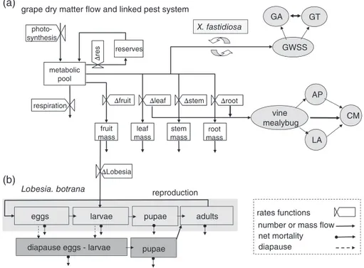
reserves fruit mass leaf mass stem mass root mass photo-synthesis metabolic pool
respiration Δfruit Δleaf Δstem Δroot
Δ
res
grape dry matter flow and linked pest system
(a)
(b) ΔLobesia
eggs larvae
Lobesia. botrana
pupae adults
diapause eggs - larvae pupae
GWSS GT GA X. fastidiosa vine mealybug LA AP CM
number or mass flow rates functions
diapause net mortality reproduction
Figure 1 Grapevine-Lobesia botrana system. (a) Dry matter flow in grapevine (Gutierrez et al., 1985; Wermelinger et al., 1991) and (b) the linkage of L. botrana life-stages including diapause induction and termination (Gutierrez et al., 2012). Note the linkages of two vascular feeding Hemiptera: the
vine mealybug and the glassy winged sharpshooter (GWSS) and their natural enemies and the transmission of the Pierce’s disease bacterium Xylella
fastidiosa by GWSS (Gutierrez et al., 2007, 2011).
montrouzieri (Gutierrez et al., 2007), as well as the glassy
winged sharpshooter (GWSS) Homalodisca vitripennis that vectors the pathogenic bacterium Xylella fastidiosa caus-ing Pierce’s disease and the two egg parasitoids Gonatocerus
ashmeadi and G. triguttatus that attack it (Gutierrez et al., 2011).
In the present study, the PBDMs for grapevine and L. botrana (Gutierrez et al., 2012) were used to analyze the effects of observed weather and a +1.8 ∘C climate change scenario on the dynamics of the system in the grape growing areas of the Palearc-tic region of Europe, Eurasia and the Mediterranean Basin.
Materials and methods
The system model for grapevine and L. botrana
A distributed-maturation time population dynamics model (Manetsch, 1976; Vansickle, 1977) (see Appendix) is used to capture the time-varying age-structured dynamics of the subcomponent populations of the grapevine/L. botrana system (see below). Biodemographic functions (Gilioli et al., 2016) are used to describe the weather-driven biology of grapevine and L. botrana that constitute the PBDMs for the species when embedded in the dynamics models. An extant PBDM model for grapevine phenology, dry matter growth and development [Wer-melinger et al., 1991 (var. Pinot Noir); Gutierrez et al., 1985 (var. Chenin Blanc)] and a PBDM for L. botrana (Gutierrez
et al., 2012) were used in the present study. Other grape varieties
were studied by Gutierrez et al. (1985) who found that Chenin
Blanc had the highest yields, followed closely by Pinot noir and Zinfandel, with Cabernet sauvignon producing 50% of Chenin
Blanc yield. Numerous varieties occur across the Palearctic region, although we use the parameters for Pinot noir as the standard. Grape yield also vary with vine age, soil, agronomic practices and other factors (Winkler et al., 1974) and hence our estimates of yield are heuristic. Only a brief description of the grapevine model is given below, whereas the biodemographic functions for L. botrana are discussed in detail.
The system model for grapevine and L. botrana is modular and consists of 13 {n = 1, … ,13} linked age-structured popu-lation dynamics models that may be in units of numbers or mass. The grapevine model consists of subunit models for the mass of leaves {n = 1}, stem {2}, shoots {3} and root {4} and the mass and number of fruit clusters {5, 6}. The submodels for L. botrana consist of age-structured population models for nondiapause and diapause immature stages respectively (e.g. eggs {7, 8}, larvae {9, 10} and pupae {11, 12}) and nondiapause adults {13}. The underpinning modelling concepts are found in Gutierrez and Baumgärtner (1984) and Gutierrez (1992, 1996), whereas the mathematics of the time invariant and time varying distributed maturation-time dynamics model are provided in Manetsch (1976), Vansickle (1977) and DiCola et al. (1999). A brief review of the mathematics is given in the Appendix. The model is driven by daily weather (see below) and the time step for each dynamics model is a day of variable length in physiological time units as appropriate for the species and/or stage. The system model was coded in the programming language Borland Delphi Pascal.
Grapevine. The grapevine model captures the phenology of
0 10 20 30 eggs/female d -1 age (days at 25°C) temperature (°C) 0 0.2 0.4 0.6 0.8 1 proportion dying egg-larvae pupa egg-larvae 0 0.04 0.08 0.12 0.16 (a) (b) (c) (d) temperature (°C) 1/days pupae 0 0.2 0.4 0.6 0.8 1 0 normalized eggs/female 0 5 10 15 20 25 30 0 5 10 15 20 25 30 35 40 0 4 8 12 16 20 24 28 32 36 16 20 24 28 32 temperature(°C)
Figure 2 The thermal biology of Lobesia botrana. (a) The rate of development of the egg-larval ( ) and pupal ( ) stages on temperature (data from Brière & Pracros, 1998), (b) the per capita oviposition profile on female age in days at 25 ∘C (data from Baumgärtner & Baronio, 1988), (c) the effects of temperature on normalized gross fecundity (data from Gabel, 1981) and (d) the proportion dying during the egg-larval and pupal periods on temperature (computed from Briolini et al., 1997). All functions are fits to data from the literature (Gutierrez et al., 2012).
as the dry matter growth and development of vegetative and fruit subunits. The production and allocation of dry matter in grapevine is depicted in Fig. 1(a), whereas the flow via feeding to L. botrana is illustrated in Fig. 1(b). Water (irriga-tion) and nutrients are assumed to be nonlimiting and hence only daily maximum–minimum temperature and solar radiation (MJ/m2/day) drive developmental and dry matter growth of the vine model. The lower thermal threshold for grapevine is 10 ∘C. Full details of the grapevine model are provided in Wermelinger
et al. (1991; see also Gutierrez et al., 1985) and hence the model
is not reviewed further.
The top-down effect of L. botrana feeding on dry mat-ter allocation and growth in grapevine is small, although the economic damage caused by larval grazing on maturing berries may be large and possibly be exacerbated by the action of the grey mold fungus Botrytis cinerea (Sclerotiniaceae) (Savopoulou-Soultani & Tzanakakis, 1988) that increases with
L. botrana infestation levels (Fermaud & Giboulot, 1992). A
mechanistic model for B. cinerea on grapevine was recently reported by González-Domínguez et al. (2015) that accounts for conidia production on various inoculum sources and for multiple infection pathways. Using discriminant function anal-ysis, the ability of the model to predict mild, intermediate and severe epidemics of B. cinerea was evaluated. The effects of
Botrytis are not included in the model, although the model of
González-Domínguez et al. (2015) can be added to our grapevine system model.
Important bottom-up plant effects on L. botrana include the phenology and abundance of fruit stages and their effects on larval-pupal developmental rates and on adult fecundity and longevity (see below).
The biology of L. botrana on grapevine. Lobesia botrana
over-winters as diapausing pupae in the crevices of vine bark, with adults emerging in spring during a period that overlaps with the development of grapevine inflorescence. Two to three genera-tions occur per year in most areas of Europe with a partial or com-plete fourth generation accruing in warmer areas (Tzanakakis
et al., 1988). Four and five generations occur in hotter areas of
Spain (Martin-Vertedor et al., 2010). Larvae of the first genera-tion damage grapevine inflorescences, with those of subsequent generations damaging green, ripening and mature berries. In late summer and autumn, L. botrana produces diapause pupae that overwinter and complete development the next spring, when they emerge as new adults (Deseö et al., 1981).
Biodemographic functions describe the developmental rates and fecundity as affected by temperature and larval diet (berry stage), diapause induction and termination, and temperature-dependent mortality (Thiéry et al., 2014). Age-specific mor-tality as a result of temperature and other factors occurs in all life stages. The data from the literature used to formulate and parameterize the biodemographic models were of varying levels of completeness, and re-interpretation of some of the data was required. Most of the functions were first reported by Gutierrez
et al. (2012) and are reproduced here for completeness (Fig. 2).
Biodemographic functions for L. botrana (Gutierrez et al., 2012)
The model can be developed using proportional rate of devel-opment but, for ease of field applications, time (t) in the model is chronological days (d), whereas age and most rates
in the biodemographic functions are in physiological time units (see below).
Rate of development. Development (aging) within a stage and
the transitioning between life stages (e.g. larvae to pupae) is not only temperature-dependent, but also may be influenced by larval diet. Data on the developmental times in days for the pre-imaginal stages reared on artificial diet at several tempera-tures were reported by Gabel (1981), Savopoulou-Soultani et al. (1996) and Brière and Pracros (1998). The extensive data on egg-larval and pupal development in Brière and Pracros (1998) were used to estimate the developmental rate at temperature
T. We aggregated the egg-larval data to reduce the variability
introduced by the fact that a daily observation interval at higher temperatures is long relative to the developmental times of the egg stage. Parsimonious Eqn (1) (cf Brière et al., 1999) was fit-ted to the developmental rate data Rs(T) = 1/d(T) at temperature
T for the egg-larval (subscript e-l) and pupal (p) stages (s = e-l, p), where d(T) is the average developmental time in days (d) on
diet at temperature T (Fig. 2a):
Rs(T) = a(T −𝜃L ) 1 + bT−𝜃U (1) Re−l(T) = 0.00225 (T − 8.9) 1 + 5T−33 (1i) Rp(T) = 0.00785 (T − 11.5) 1 + 4.5T−33 (1ii) The variables𝜃Land𝜃Uare the lower and upper thermal thresh-olds, whereas a and b are constants. Specifically,𝜃Land𝜃U for the e-l stage are 8.9 and 33 ∘C, respectively (Eqn (1i)), whereas values for the pupal stage (p) are 11.5 and 33 ∘C (Eqn (1ii)). The upper threshold𝜃Uis approximately the temperature where the function begins declining to zero. Data on adult female longevity were available only at 25 ∘C (Baumgärtner & Baronio, 1988) and, assuming the developmental thresholds for pupae, the adult developmental rate is scaled as Radult(T(t)) = 0.77Rp(T(t)) (Gutierrez et al., 2012). On artificial diet, Rs(T(t)) is the pro-portion of development of a stage that occurs at temperature
T(t) at time t and, hence, for individuals entering stage s at age x = 0 at time t = t0, development on average is completed when
t
∑
t0
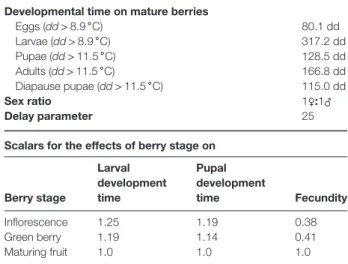
Rs(T (t)) = 1. In the model, developmental times of cohort members have a characteristic mean and distribution (Fig. A1b). Developmental times in degree days [Δs(diet) = d(T) · (T −𝜃L)] on artificial diet were computed for all stages in the linear range of Rs(T): eggs (Δe= 80.1dd>8.9 ∘C), larvae (Δl= 317.2dd>8.9 ∘C), pupae (ΔP= 128.5dd>11.5 ∘C) and adult longevity (ΔA= 166.8dd> 11.5 ∘C) (Table 1). During late summer
to autumn, increasingly, larvae developing on mature berries become diapause pupae that have an approximately 15% lower mean developmental time in spring compared with nondiapause pupae (i.e. Δdiap= 0.85Δp) (Gutierrez et al., 2012).
Larval and pupal developmental times on diet differ from field values, which vary with host fruit stage (frt) (Savopoulou-Soultani et al., 1999; Torres-Vila et al., 1999).
Table 1 Parameters for the Lobesia botrana model Developmental time on mature berries
Eggs (dd> 8.9 ∘C) 80.1 dd Larvae (dd> 8.9 ∘C) 317.2 dd Pupae (dd> 11.5 ∘C) 128.5 dd Adults (dd> 11.5 ∘C) 166.8 dd Diapause pupae (dd> 11.5 ∘C) 115.0 dd Sex ratio 1♀:1♂ Delay parameter 25
Scalars for the effects of berry stage on
Berry stage Larval development time Pupal development time Fecundity Inflorescence 1.25 1.19 0.38 Green berry 1.19 1.14 0.41 Maturing fruit 1.0 1.0 1.0
As a standard, larval and pupal times on mature berries are approximately 10% shorter than on diet (Gabel & Mocko, 1984) (see Supporting information, File S1) and average larval developmental times on inflorescence and green berries are 1.25- and 1.19-fold longer than on mature berries, whereas those for pupae are 1.19- and 1.14-fold longer (Table 1). Hence, in the model, the corrections [𝜑l(frt)] for larval developmental times on inflorescence, green berries and mature berries are 1.125 (= 0.9 × 1.25), 1.07 (= 0.9 × 1.19) and 0.9, respectively, and those for pupae [𝜑p(frt)] are 1.07, 1.026 and 0.9. The
within season changes in stage developmental times are easily accommodated using the time-varying form of the distributed maturation-time population dynamics model (Vansickle, 1977) (see Appendix).
Ignoring the time variable t, the daily increment of aging [Δxs(T, frt)] of larval and pupal stages (subscript s = l, p) in dd at temperature T is:
Δxs(T, frt) = 𝜑s(frt) · Rs(T) · Δs(diet), (2i) whereas ageing in the egg and adult stages depends only on temperature (Eqn (2ii)):
Δxs(T (t)) = Rs(T (t)) · Δs(diet). (2ii) Note that Rs(T(t)) in Eqns (2i) and (2ii) corrects for the nonlinearity of development with T and further changes in physiological time are not always equal to the change in age [i.e. Δt(T(t)) = (T(t) −𝜃L)≥ Δx(T(t)) ≥ Δx(T(t), frt)]. Lastly,
average temperatures in the grape canopy are approximately 3.7% lower than ambient (cf Potter et al., 2013).
Reproduction. Observed average per capita fecundity ranges
from 120 eggs on grapevine to 170 on an artificial diet, although higher fitness may occur on some wild hosts (e.g. the evergreen shrub Daphne gnidium L.) in the Mediter-ranean region (Thiéry & Moreau, 2005; Maher & Thiery, 2006). Per capita age-specific oviposition rate on grapevine [eggs female−1d−1= F(t, x, T, diet
female age (x) (Baumgärtner & Baronio, 1988) (Fig. 2b), tem-perature (T) (Gabel, 1981) (Fig. 2c) and the diet (i.e. fruit stage) of the larvae producing the adult female (Savopoulou-Soultani
et al., 1999; Torres-Vila et al., 1999; Moreau et al., 2016). We
characterize the per capita age-specific fecundity profile [f (x)] of adults of age x at 25 ∘C using the function proposed by Bieri
et al. (1983), the effect of temperature on fecundity is captured
by a concave function [0≤ 𝜙(T(t)) ≤ 1 ] in the favourable range [Tmin= 17∘C, Tmax= 32∘C] and the effects of fruit stage are cap-tured by the step function𝜓(frt) (Table 1; Gutierrez et al., 2012).
F(x, t, T, frtl ) =𝜓 (frt, t) · 𝜑 (T (t)) · f (x) , (3i) where f (x) =28.5 (x − 1) 1.5x−1 at T = 25∘C 𝜑 (T (t)) = 1 − [ ( T − Tmin− Tmid ) Tmid ]2 , with Tmid=(Tmax− Tmin)∕2 = 7.5∘C.
𝜓(frtl ) = ⎛ ⎜ ⎜ ⎜ ⎝ 0.31 (inflorescence) 0.48 (green berries) 1 (maturing fruit) .
Sex ratios (sr) vary widely on different hosts with 0.82:1.18 (♀:♂) and 1.02 : 0.98 (♀:♂) reported using stock culture insects raised on artificial diet supplied with plant material from grape varieties Cabernet sauvignon and Red Bacco, respectively (Thiéry & Moreau, 2005). In a similar study, Thiéry et al. (2014) found a 1 : 1 ratio on six varieties of grape. We use sr = 0.5 in the model; hence, the total egg-load [E(t, T, dietl)] by all females of age x = 0 to xmaxat time t is:
E(t, T, frtl ) = sr ∫ xmax x=0 N (x, t) F(x, t, T, frtl ) dx, (3ii) where N(x,t) is the number of adults of age x at time t. The eggs are deposited singly in berry clusters, and the adult search for oviposition sites is imperfect and affects realized fecundity. This search behaviour is captured by the functional response model (Eqn (A2)).
Temperature-dependent mortality. The total mortality during the
egg-larval and pupal stages varies with temperature (T) (Fig. 2d) (Eqn (4i)), with data from Briolini et al. (1997):
0≤ 𝜇s(T) = cs ( T − Tm Tm )2 ≤ 1 (4i)
The constants in Eqn (4i) are: Tm= 21.5 ∘C and cs
= {
2.2 for eggs and larvae 2.0 for pupae and adults.
In the model, we must convert the stage mortality rate𝜇s(T) to a daily mortality rate [Δ𝜇s(T(t))] and hence we multiply by the proportion of the stage completed during time t:
0≤ Δ𝜇s(T (t)) =𝜇s(T (t))
Δxs(T (t))
Δs(t) ≤ 1 (4ii)
Andreadis et al. (2005) estimated the super cooling point for diapause and nondiapause pupae as −24.5 and −22.5 ∘C, respectively, although most pupae die at subzero temperatures well above the super cooling point. Hence, in the absence of sound data, we assume the same mortality rate on temperature for both pupal forms.
Other sources of mortality. Extrinsic mortality occurs as a result
of generalist natural enemies, host stage suitability, larval dis-persal and other factors, although field life-table data to estimate these factors for L. botrana are generally unavailable. In heavily parasitized vineyards, larval mortality during spring/summer may reach 80% and up to 90% mortality may occur during pupal diapause (Marchesini & Dalla Montà, 1994; Xuéreb and Thiéry 2006). Gabel and Roehrich (1995) showed a bimodal pattern in berry stage preference for feeding, with intermediates stages being unsuitable for larval survival. Torres-Vila et al. (1997) found that dispersal distance in L. botrana larvae increased with larval density, although the mortality rates were the same. Gilioli
et al. (2016) estimated mortality rates in L. botrana using
unpub-lished field population dynamics data and the Manly (1989) simulation estimation approach, although the results are time and place specific, and sampling errors from various sources affected the field data. Lanzarone et al. (2017) used Bayesian methods to estimate the mortality using the same data and, although the fits were better, the method requires field data to implement and hence is not general. Hence, to keep larval populations within relative bounds (< 70 larvae per vine), we used a variant of the Nicholson and Bailey (1935) model, where ignoring the time variable t, the aggregate extrinsic mortality [0< 𝜇c(·)< 1] is assumed to increase with both temperature [i.e. Δt(T) = dd>8.9 ∘C] and pest density (Neggs+ NLarvae) but at a decreasing rate (Eqn (5)).
0≤ 𝜇c(·) = 1 − e−0.0002Δt(T)(Neggs+Nlarvae) < 1 (5) The constant 0.0002 is arbitrary and when multiplied by Δt(T) estimates the fraction of the population that may be found at temperature T. Thus, 𝜇c(·) affects egg-larval abun-dance, although it does not affect the phenology of the life stages. Hence, we caution that the predicted abundance of L.
botrana life stages can only be viewed as a metric of
over-all favourability of weather at each lattice location. A similar composite model was used with good success in predicting the geographical range and relative abundance of the exotic light brown apple moth Epiphyas postvittana in California that is attacked by a suite of native generalist natural enemies (Gutierrez
et al., 2010).
All sources of intrinsic and extrinsic mortality are combined and enter the dynamics model as a net proportional age-specific loss rate (i.e.𝜇iin Eqn (A1)).
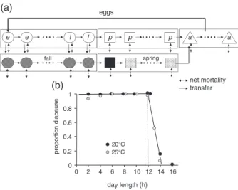
Diapause. Deseö et al. (1981) reported that L. botrana has a
facultative autumn-hibernal type I diapause that with decreas-ing short-day photoperiods (dl) durdecreas-ing autumn increasdecreas-ingly induces egg and early larval stages to become diapause pupae (Tzanakakis et al., 1988). In the model, eggs and larvae destined
e e l l p p p a a spring fall 20°C 0 0.2 0.4 0.6 0.8 1 0 2 4 6 8 10 12 14 16 day length (h) proportion diapaus e (a) (b) 25°C eggs net mortality transfer
Figure 3 Submodel for diapause induction. (a) Age-structured models for the dynamics of nondiapause (open symbols) and diapause (dark stip-pled symbols) egg (e), larval (l), pupal (p) and adult (a) stages with flow from nondiapause age classes to same age diapause classes. Devel-opment of diapause eggs and larvae continue until they become first stage diapause pupae (black square) that, in spring, begin development (light stippled squares) to emerge as adults (for further explanation, see text). (b) The proportion of the eggs-larvae that will enter diapause on day length when reared at 20 or 25 ∘C (data from Roditakis & Karandinos, 2001).
to become diapause pupae flow (Fig. 3a, solid arrows) from non-diapause cohorts (Fig. 3a, open circles) to the same age non-diapause cohorts (Fig. 3a, closed stippled circles) where they continue development to pupation (Fig. 3a, black square). Diapause pupae remain quiescent until increasing temperatures during late winter and spring stimulate post-diapause development (Fig. 3a, stip-pled square) leading to adult emergence (Fig. 3a, bent upturned arrow) and oviposition. During autumn, larvae not entering dia-pause continue normal development to the adult stage and ovipo-sition if hosts are available. After a short pre-ovipoovipo-sition period, newly emerged adult females from all sources deposit eggs that enter the first age class of the egg stage. The dashed double arrows indicate the net age-specific mortality rate (𝜇i) in substage (i) as a result of all causes.
Two biodemographic models for diapause induction in
L. botrana are available. The first is based on laboratory studies
by Roditakis and Karandinos (2001) who exposed eggs and larvae to several diel and nondiel photoperiods at 20 and 25 ∘C and found that diapause is increasingly induced at day length (dl) below 14.15 h at both temperatures (Fig. 3b). Collapsing the data across the two temperatures yields Eqn (6i) (0≤ diap(dl) ≤ 1):
diap (dl) = ⎧ ⎪ ⎨ ⎪ ⎩ 0 for dl> 14.15h 0.4565 × (14.15 − dl)≤ 1 for dl ≤ 14.15h (6i) The second model is based on the observation by Riedl (1983) in codling moth of a north–south gradient for diapause induction, which Baumgärtner et al. (2012) explored for L. botrana using field data from across several locations across Europe. They
found that dl and latitude (lat) affected the diapause induction rates (diap(dl, lat)) (Eqn (6ii)):
0≤ diap (dl, lat) = 4.487 + 0.056lat − 0.4565dl ≤ 1, (6ii) Diapause models 6i and 6ii give qualitatively similar results (see Supporting Information, File S1) but, because of uncertainty in the field data and in fitting model Eqn (6ii), we use the simpler model (Eqn (6i)). The daily rate of diapause induction in eggs and young larvae (Δdiape − l(dl, T)) is:
0≤ Δdiap (dl, T)e−l= diap (dl) · Δxe−l
Δe−l ≤ 1, (6iii) where Δxe − lis the change in age in degree days at temperature
T at time t, and Δe − l is the egg-larval developmental time in
dd> 8.9 ∘Con mature berries.
Emergence from diapause. The phenology and population
dynamics of L. botrana vary with weather across locations and years. As temperatures rise above 11.5 ∘C in late winter and spring, diapause pupae begin development, yielding the first generation of new adults. Assuming a normal distribution, 95% of the diapausing pupae would be expected to emerge in 2 SDs from the mean. If the average developmental time of diapause pupae is Δdiap= 115dd>11.5 ∘C, then, from the definition
of Erlang parameter k = Δ2
diap∕var in our distributed maturation time dynamics model, and assuming a conservative value of
k = 25 and the std =√var = 23dd>11.5 ∘C (see Appendix), the 2 SD window for emergence is 69dd>11.5 ∘C to 161.2dd>11.5 ∘C. This approach worked well for modelling field data collected in the Napa Valley of California (Gutierrez et al., 2012) and it is used here.
Weather data
Ambient daily weather data (maximum and minimum tem-perature, rainfall and solar radiation (MJ/m2/day) from the AgMERRA global weather dataset for the period 1 January 1980 to 31 December 2010 for 17 854 lattice cells (of approx-imately 25 × 25 km) for Europe and the Mediterranean Basin were used. Because of computational constraints (approximately 24–30 h per run on a laptop copmputer), only alternate lattice cells (i.e. 4506) were used to run the PBDMs. This coarser grain analysis does not affect the patterns or conclusions and is closer to the original spatial resolution of the underlying temperature data used to assemble the AgMERRA data set (Ruane et al., 2015). The AgMERRA data are a daily time series of maximim–minimum temperatures, solar radiation, rainfall and relative humidity at an approximately 25-km geographical resolution for the period 1980–2010 (National Aeronautics & Space Administration, 2015; NASA). It was created as a base-line forcing dataset for the Agricultural Model Inter-comparison and Improvement Project (AgMIP; http://www.agmip.org/; Ruane et al., 2015). This dataset was produced by combining a state-of-the-art reanalysis of weather observations (Modern-Era Retrospective analysis for Research and Applications, MERRA; Rienecker et al., 2011) with observational datasets from
2008 larvae 100 100 150 200 250 0 50 100 150 n. of larvae 2008 50 0 (a) 2009 larvae 150 200 250 150 200 250 100 0 100 200 300 n. of larvae 2009 days 50 0 (b) 100 150 200 250
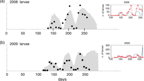
Figure 4 Scaled simulation of Lobesia botrana larval densities (grey) compared with field data (•) from Colognola ai Colli (Veneto region, Italy) for the (a) 2008 and (b) 2009 seasons (redrawn with persmission from Gilioli et al., 2016). Inset: data (x) and simulation (blue line) from Gilioli et al., 2016. [Colour figure can be viewed at wileyonlinelibrary.com].
in situ observational networks and satellites (Ruane et al.,
2015). The AgMERRA data are used as the observed weather for the recent past.
The effects of projected climate warming on grapevine and
L. botrana across the Palearctic region were examined by
comparing climate model projections of the changes from a base period of 1960–1970 with a future 2040–2050 period (i.e. a climate change scenario). In the present study, we used the A1B regional climate change scenario that posits +1.8 ∘C warming for the Euro-Mediterranean region (Dell’Aquila et al., 2012). The A1B scenario is towards the middle of the IPCC (2014) range of greenhouse gas (GHG) forcing scenarios (Giorgi & Bi, 2005). The uncertainty associated with climate model predictions forced using the A1B scenario is low for the Mediterranean region relative to the rest of the globe (Gualdi et al., 2013). This fine scale weather dataset at an approximately 30-km resolution was developed by Dell’Aquila et al., 2012 using the regional climate model PROTHEUS (Artale et al., 2010) to refine and rescale the coarser (approximately 200-km resolution) global climate simulation forced with observed GHG for years 1951–2000 and the IPCC (2014) A1B GHG emissions scenario for 2001–2050. PROTHEUS is a coupled atmosphere–ocean regional model that allows simulation of local extremes of weather via the inclusion of a fine scale representation of topography and the influence of the Mediterranean Sea (Artale et al., 2010). The PROTHEUS A1B scenario is a finer scale projection of future climate change for the Euro-Mediterranean region and was used to run the grapevine/L. botrana system across the Palearctic region for the periods 1960–1970 and 2040–2050.
Data, simulation and GIS analysis
Batch files were used to initialize and run the model across all locations for the period of available weather data. The different species in Fig. 1 can be included in any run of the model using true-false Boolean variables from a batch file. The starting day for all runs was 1 January of the first year with an initial density
of four diapause pupae plant−1 (area = 2.3 m2) assumed at all locations. Although the model predicts the density of grapevine subunits and all stages of L. botrana, we used the average annual yield per vine and the annual sum of L. botrana pupae per vine per year as the metrics of favourability for grape and of
L. botrana infestation levels, respectively. The simulation data
on a per vine basis were georeferenced and written to batch files by year for mapping and analysis. Because the model must equilibrate to the effects of local weather from the common initial conditions, the results for all simulation runs in the first year were not used to compute lattice cell averages, SDs and coefficient of variations as a percentage (CV).
The open source GIS GRASS originally developed by the United State Army Corp of Engineers was used to map the data using bicubic spline interpolation on a 3-km raster grid. The version of GRASS used is maintained and further developed by the GRASS Development Team (2014) (http://grass.osgeo.org).
Results
Figure 4 compares the scaled model predictions and field dynam-ics data for L. botrana larvae reported by Gilioli et al. (2016; inset figures) from Colognola ai Colli (Veneto Region, Italy) during 2008 and 2009 for days 100–265. Weather data from the nearest AgMERRA cell to Colognola ai Colli were used in the simula-tion. The goal was to gauge how well the model captured the phenology of L. botrana and not to make precise predictions of densities that are affected by net immigration from other hosts, grape cultivar, daily weather, predation, sampling error, etc. (see Supporting information, File S1). Larvae were detected earlier in 2009 than in 2008 with the largest discrepancies between the field data (•) and the simulation (the shaded area) in the present study (see Fig. 4) and in Gilioli et al. (2016) occurring during late sea-son beyond the last field sampling date of day 265. Harvest dates vary between years and for different varieties and, in the model, occur at approximately 1850–1900dd>10 ∘C(e.g. ∼day 290). Note
0 500 1000 1500 2000 2500
3000 Near Cordoba, Andalucía, Spain
g dr y ma tt er/vine berries leaf shoot root reserve 0 10 20 30 0 5 10 15 20 25 adults diap. pupae eggs larvae pupae 2010 number /vine
(b)
2006 2007 2008 2009(c)
(a)
Figure 5 Simulation of the grapevine system dynamics near Cordoba (Andalucía region, Spain) (longitude −4.375, latitude 37.875) during 2006–2010. (a) Phenology of grapevine dry matter allocation dynamics, (b) dynamics of adult Lobesia botrana diapause pupae and adult dynamics and (c) the dynamics of egg production, larvae and nondiapause pupae.
that decreasing adult longevity 25% tightens the fit considerably (see Supporting information, File S1).
Simulated grapevine and L. botrana dynamics near Cordoba (Andalucía region, Spain)
For heuristic purposes, we use 2001–2010 weather data from a lattice cell near Cordoba (Andalucía region, Spain) (longitude −4.375, latitude 37.875) to illustrate the richness of the model output computed for all 4506 lattice cells. The full dynamics of the plant subunit population growth are shown in Fig. 5(a) (Wermelinger et al., 1991), whereas the dynamics of L. botrana life stages are illustrated in Fig. 5(b, c). The adult dynamics in Fig. 5(b) show the number of overwintering pupae (dark area) and the cumulative emergence of adult males and females. Figure 5(c) depicts the pattern of oviposition by reproductive adults of the different generations (Fig. 5c, shaded area) and the larval and pupal dynamics.
Adult generations per year
In Europe, more generations occur in hotter areas (e.g. Spain) (Martin-Vertedor et al., 2010) than in cooler areas. We demon-strate this by simulating adult dynamics at six locations in Spain along the −4.375∘ longitude at different latitudes during 1990–2010 (Fig. 6). The first peak each year is the emergence of adults in spring and the subsequent ones are summer genera-tions. The number of generations at each location varies between
years as a result of weather conditions, with the relative number of generations given as appropriate. The fewest generations (two to three) are predicted for the mountainous areas of Cantabria in Northern Spain and increase to four to five generations in the northern parts of Andalucía near Cordoba.
A regional analysis of Europe and the Mediterranean Basin System dynamics using observed 1980–2010 weather data.
Figure 7(a,d) shows the prospective distribution of average annual grapevine yield and average L. botrana pupal density dur-ing the period 1980–2010 in the area of known grape production in the Palearctic region estimated from Monfreda et al. (2008) (see Supporting information, File S1). Highest yields occur in a broad band around 40∘N latitude extending from Spain–Portugal in the west to Turkey in the east. The frequency distribution of average yield (Fig. 7b) shows a relative range 0–3500 g dry mat-ter per plant. The CV as a percentage (Fig. 7c) also increases northward in response to colder more variable seasons and south-ward as a result of increasing high temperatures that affect yield. A high average yield and a low coefficient of variation for annual yield at each location characterize the region of highest favoura-bility for grapevine.
Total annual pupal density and low CV are also metrics of climatic favourability for L. botrana at each location. Highest average density and low CV are predicted throughout the major regions of grape production (Fig. 7d–f). The highest CVs are predicted in Egypt and in colder northern areas.
Figure 6 Simulated adult Lobesia botrana dynamics at six locations in Spain along the −4.375∘ longitude at different latitudes during years 1990–2010. The first dark peak in each year is the spring generation.[Colour figure can be viewed at wileyonlinelibrary.com].
(a) (b) (c)
(d) (e) (f)
Figure 7 Prospective simulation of the grapevine/Lobesia system in the Palearctic region below 1500 m a.s.l during 1980–2010. (a) The distribution of average grape yield. (b) Frequency distribution of the number of lattice cells with different yield. (c) Coefficient of variation of yield as a percentage. (d) Distribution and abundance of Lobesia botrana pupal density. (e) Frequency histogram of cells with different pupal densities. (f) Coefficient of variation of pupal density as a percentage.
(a) (b) (c)
(d) (e) (f)
Figure 8 Prospective simulation of the grapevine/Lobesia system in the Palearctic region below 1500 m a.s.l. assuming a 1.8 ∘C increase in temperature during 2040–2050 (scenario A1B). (a) The distribution of average grape yield. (b) Histogram of the number of lattice cell with different yield. (c) Coefficient of variation of yield as a percentage. (d) Distribution and abundance of Lobesia pupal density. (e) Histogram of cell with different pupal densities. (f) Coefficient of variation of pupal density as a percentage.
System dynamics with +1.8 ∘C climate warming (A1B scenario).
The yields under projected +1.8∘C climate warming during 2040–2050 (IPCC, 2014, A1B GHG scenario) in the cur-rent Palearctic area of grapevine distribution are illustrated in Fig. 8(a). Regression of annual dd> 10 ∘Cunder the A1B scenario on those for the 1960–1970 baseline period shows a cumu-lative increase in physiological time of approximately 18.5% [dd>10C , A1B= 1.185dd>10C , base, R2= 0.993].
The effects of climate warming can be viewed by comparing average yields during the 2040–2050 period and the 1980–2010 period yields (Fig. 8a versus Fig. 7a). Specifically, average yield in currently favourable areas increases by approximately 10% as a result of climate warming; the range of favourability expands into more northern areas and higher elevations; the favourable geographical range declines with increasing CV in warmer North Africa and the Middle East (Fig. 8c versus Fig. 7c). Similarly,
L. botrana pupal densities increase with climate warming in
the areas favourable for grapevine, especially in areas of Spain, Greece and Turkey, but decline in areas of the Middle East (Fig. 8d versus Fig. 7d).
The effects of climate warming on the system dynamics across the region are best seen by plotting the difference between yields and pupal densities predicted using the IPCC A1B GHG scenario for 2040–2050 and those predicted for the baseline period 1960–1970 (Fig. 9a,c). Roughly, the largest increases in yield with climate warming are predicted in higher latitudes and elevations of Spain, Italy, southern France and in Turkey in the band around 40∘N latitude and, to a lesser extent, northward in Europe where conditions for grapevine improve. Yields are unchanged or lower in areas of the Middle East and parts of North Africa. Plots of yields under the A1B scenario on the
base years 1960–1970 do not give a meaningful relationship (see Supporting information, File S1). However, using the same colour schema as in Fig. 9(a), the frequency distribution of changes in yield (Fig. 9b) shows a comparatively larger area with increased yield across the region than with yield declines.
Increases in L. botrana pupal abundance occur throughout a wide part of the region because warmer temperatures allow additional generations of the moth to develop (Fig. 9c). This change is best visualized by the frequency histogram of predicted change (i.e. Δpupae in Fig. 9d). A plot of Δyield on Δpupae (Fig. 9e) shows that L. botrana pupal densities not only increase in areas favourable for yield increases (+, +), but also in areas of yield decrease (−, +) (upper half quadrants). Pupal abundance may decrease in areas where yields decrease (lower left quadrant; −, −), although abundance never decrease in areas with yield increases (lower right quadrant; +, −).
Discussion
Grape is a mainstay cultural, economic and ecological factor of Mediterranean Basin and is the fruit crop with the largest acreage and the highest economic importance globally (Vivier & Pretorius, 2002). Grape and its pests have been the subject of considerable research efforts. Controlling infestation levels of the polyphagous grapevine moth has a high priority and several models have been developed for use in IPM decision support (Baumgärtner & Baronio, 1988; Briolini et al., 1997; Schmidt
et al., 2003; Severini et al., 2005; Gilioli et al., 2016; Lanzarone et al., 2017). In the present study, we used a weather-driven
PBDM for grape vine and L. botrana that was developed based on European data and initially used to assess the invasiveness
Δ pupae Δ g yield 2000 -1000 0 -2000 1000 Δ g yield cells × 103 0 5 10 15 20 0 10 20 30 50 40 Δ pupae cells × 103 20 -30 -20 -10 0 10 -40 -50
+ +
- +
+
-- --
-45 -35 -25 -15 -50 5 15 25 -2000 Δ yield 2000 (e) Δ pupae (a) (c) (d) (b)Figure 9 Comparison of prospective changes in the grapevine/Lobesia system in the Palearctic region below 1500 m a.s.l. given an A1B scenario of 1.8 ∘C average temperature increase between 2041–2050 (future) and 1960–1970 (baseline) simulated weather data. (a) The distribution of average changes in grape yield. (b) Histogram of the number of lattice cells with different levels of yield changes. (c) The distribution of average changes in the abundance of Lobesia botrana pupal density. (d) Histogram of cells with different levels of changes in pupal densities. (e) Plot of changes in yield (Δyield) on changes in pupal density (Δpupae).
and potential distribution and relative abundance of L. botrana in California after its accidental introduction in 2009 (Gutierrez
et al., 2012). Because the PBDM is mechanistic and weather
driven, it may be applied to any regions where grape is grown. The model was used to examine the favourability of observed weather for grape and L. botrana across the grape growing regions of the Palearctic, as well as to examine how favourability would change in the face of climate warming.
PBDMs are perceived to be difficult to develop, although this is not the case given an understanding of the biology and the simple mathematics of the population dynamics models and the availability of sound biological data (Gutierrez & Ponti, 2013). PBDMs may be viewed as time-varying life tables (sensu Gilbert
et al., 1976). Multitrophic systems that include the bottom up
dynamics of host plants on herbivore species and the top-down effects of higher trophic levels, as well as aspects of physiology and behavior, can be developed (Fig. 1). PBDM modelling of this level of complexity is facilitated by the fact that the same dynamics model are used for all species and the same forms for the biodynamic models reoccur for analogous processes in the life histories of all species across trophic levels (Gutierrez & Baumgärtner, 1984; Gutierrez et al., 2011; Gutierrez & Ponti,
2013). The development of PBDMs is facilitated by their mod-ular structure enabling different combinations of species to be implemented in model runs using simple true-false Boolean vari-ables, allowing the system to be viewed from the perspective of any of the interacting species (Gutierrez & Baumgärtner, 1984; Gutierrez & Ponti, 2013). The inclusion of rich biology allows prediction and mapping of the phenology, dynamics and rela-tive abundance across a wide landscape with varied climates and future climate change. When the requisite biological data are not available, the model structure provides a useful guide for identifying the data gaps (Ponti et al., 2015) facilitating efficient gathering of the missing data to characterize the biodemographic functions and to make preliminary estimates of the pest dynam-ics. In the best case, PBDMs can be tested against field data (Rodríguez et al., 2013). The PBDM approach in a GIS con-text has been applied to many agroecological systems (Gutierrez
et al., 2006, 2007, 2010, 2011, 2015, 2016; Ponti et al., 2014) and
has provided considerable insights concerning the biology at the local and regional level useful in developing pest management practices and policy (see below). However, despite their consid-erable utility, we caution that all models including PBDMs are incomplete.
Regional dynamics of grape and L. botrana
In Europe, two distinct generations of L. botrana occur in Switzerland (Moraviea et al., 2006), although three or even four may occur in southern Europe (Bovey, 1966; Gabel & Mocko, 1984; Milonas et al., 2001; Roditakis & Karandinos, 2001). Martin-Vertedor et al. (2010) found four and a half generations in western Spain with a partial fifth recorded during 2006. A similar range of generations was predicted from seven locations on a north–south gradient in California (Gutierrez
et al., 2012) and on a north–south gradient in Spain in the
present study (Fig. 6). Under nonlimiting water, the number of generations of L. botrana is determined largely by temperature and photoperiod and the availability of hosts. Studies on the spatial distribution of L. botrana in central Italy showed that its distribution among hosts is not limited to vineyards because a high presence may occur in olive groves and in other hosts not normally considered in grape pest management practices (Sciarretta et al., 2008).
Climate warming effects. Climate warming (and increased CO2
levels) will likely not only affect development of the grapevine and yield, but also higher trophic levels (Caffarra et al., 2012; Reineke & Thiéry, 2016). Because PBDMs are driven by weather, their application is not time and place specific, and they can readily be extended to examine the effects of climate change scenarios, or historical observations such as those of Martin-Vertedor et al. (2010), who found evidence that climate warming during 1984–2006 in six vine-growing areas of west-ern Spain caused earliness of adult flights of more than 12 days and increased voltinism.
To examine the effects of climate warming, we used weather data from a fine-scale regional climate model simulation (Artale
et al., 2010; Dell’Aquila et al., 2012) based on the A1B
sce-nario of intermediate climate change (IPCC, 2014) that predicts an average increase in daily temperatures of +1.8 ∘C for years 2040–2050 versus 1960–1970 across the Euro-Mediterranean region. The model predicts that grapevine yields will increase northward and in higher elevations, although they will decrease in more southern areas of the extant distribution as tempera-tures approach the upper thermal limits for grape (and where water becomes limiting). The relative abundance of L. botrana will increase generally throughout the grape growing region. In more northern areas, warmer temperatures will decrease winter mortality and increase the summer reproductive period (see Sup-porting information, File S1). By contrast, L. botrana levels may decrease in southern areas (e.g. southwestern Spain, Morocco) where high summer temperatures approach or exceed the upper thermal limits of the moth and adversely affect its vital rates (Fig. 9c). The apparent large changes in southwestern Spain and Morocco are artefacts of the insensitivity of the colour bar scale selected to illustrate the changes in the larger area of the Palearc-tic range of the moth. For this reason, the maps for the A1B 2040–2050 and 1961–1970 results are illustrated on a different scale in the Supporting information (File S1) and show that the increases and decreases in L. botrana in southwestern Spain and Morocco were mostly< 10 pupae. Similar declines in pupal den-sities are predicted for the Eastern Mediterranean region (Syria, Lebanon, Israel and Palestine).
In summary, L. botrana populations will increase as a result of climate change in most areas where grape yield increase, although levels may increase or decrease where grape yields decrease (Fig. 9e). Hence, control of L. botrana is essential, and sound PBDMs can be useful and for developing and evaluating control strategies locally and regionally, and implementing them in real time (Gilioli et al., 2016).
Control of L. botrana
Many parasitoids and predators attack L. botrana immature stages (Scaramozzino et al., 2017), although they do not pro-vide economic control (Xuéreb & Thiéry, 2006; B˘arbuceanu & Jenser, 2009) and hence ecologically sound IPM control strategies are required. The wide range of wild host plants in the Palearctic region (http://www.cabi.org/isc/datasheet/42794) complicates control. In Europe, insecticides and mating dis-rupting pheromones are commonly used for control of L.
botrana (Oliva et al., 1999; Ifoulis & Savopoulou-Soultani,
2004), although biopesticides such as Bacillus thuringiensis show promise (Ioriatti et al., 2011; Pertot et al., 2016).
The economic thresholds for insecticide control of L. botrana are qualitative, and depend on the moth generation, the suscepti-bility of the cultivar to infection by Botrytis, as well as whether the grapes are produced for table fruit or wine (Ioriatti et al., 2008, 2011). The proper timing of conventional insecticides tar-geting adult flights is critical for effective control (Caffarelli & Vita, 1988; Oliva et al., 1999; Boselli & Scannavini, 2001) and several phenological models have been developed to fore-cast the flight of the different generations of adult moths (Gabel & Mocko, 1984; Caffarelli & Vita, 1988; Del Tío et al., 2001; Milonas et al., 2001; Moraviea et al., 2006; Gallardo et al., 2009; Gutierrez et al., 2012; Gilioli et al., 2016).
In Europe, the use of pheromones for detection and control of
L. botrana by mating disruption is well developed (Harari et al.,
2007) and, unlike pesticide use, precise timing is less critical as the period of pheromone efficacy is quite long, although coverage must be continuous during the season (Anfora et al., 2008). Pheromones reduce the reproductive output of the population (Torres-Vila et al., 2002), although effectiveness depends on temperature and wind speed, rate of pheromone release, size of the target area, cultural practices, the presence of alternate host plants that serve as unregulated sources of adult moths (Vassiliou, 2009) and the slope of the land (Carlos et al., 2010). Effectiveness is inversely density-dependent and insecticide use may be required at high moth densities (Gordon et al., 2005). Good control of L. botrana has been demonstrated in Europe using pheromone applied against the flight of spring generation adults, with additional pheromone dispensers being applied starting in early June against the first and later summer flights (Anfora et al., 2008; Vassiliou, 2009; Ioriatti et al., 2011). The pheromone strategy has been most effective when applied on an area wide basis (Ioriatti et al., 2011). Simulation and marginal analysis using a PBDM for L. botrana in California predicted recommendations for mating disruption similar to those of the above field studies (see Supporting information, File S1) (Gutierrez et al., 2012). Furthermore, under climate warming, the first generation flight of adults would occur earlier and the
season would be longer with one or more additional generations, although this would not alter the underpinning pheromone-based control strategy.
Last, at the strategic level, PBDMs can be used as the production function in a bio-economic analysis of grape to assess local and regional impact of different pests, disease and control strategies under extant and climate change scenarios (Regev
et al., 1998; Pemsl et al., 2007; Ponti et al., 2014; Gutierrez et al.,
2015).
Acknowledgements
We are grateful to Dr Markus Neteler of mundialis GmbH & Co. KG (http://www.mundialis.de) and the international network of co-developers for maintaining the Geographic Resources Anal-ysis Support System (grass) software and making it available to the scientific community. We thank Ruane et al. (2015) and addi-tional colleagues of the Agricultural Model Inter-comparison and Improvement Project (AgMIP; http://www.agmip.org) for com-piling and making the weather data available. Funding for the modelling/GIS analysis was provided by the Center for the Anal-ysis of Sustainable Agricultural Systems (CASAS) and Agenzia nazionale per le nuove tecnologie, l’energia e lo sviluppo eco-nomico sostenibile (ENEA), Rome Italy. The daily weather data are from different sources. The observed weather data are from NASA (2015) and were downloaded from: https://data.giss.nasa .gov/impacts/agmipcf/agmerra. The climate change scenario is from the Climate Modelling and Impacts Laboratory, ENEA.
Supporting information
Additional Supporting information may be found in the online version of this article under the DOI reference:
10.1111/afe.12256
File S1. Supporting information for the effects of climate warming on grape and grapevine moth.
References
Ainseba, B., Picart, D. & Thiéry, D. (2011) An innovative multistage, physiologically structured, population model to understand the Euro-pean grapevine moth dynamics. Journal of Mathematical Analysis and
Applications, 382, 34–46.
Andreadis, S., Panagiotis, S., Milonas, G. & Savopoulou-Soultani, M. (2005) Cold hardiness of diapausing and non-diapausing pupae of the European grapevine moth, Lobesia botrana. Entomologia
Experimentalis et Applicata, 117, 113–118.
Anfora, G., Baldessari, M., De Cristofaro, A. et al. (2008) Control of
Lobesia botrana (Lepidoptera: Tortricidae) by biodegradable ecodian
sex pheromone dispensers. Journal of Economic Entomology, 101, 444–450.
Artale, V., Calmanti, S., Carillo, A. et al. (2010) An atmosphere-ocean regional climate model for the Mediterranean area: assessment of a present climate simulation. Climate Dynamics, 35, 721–740. B˘arbuceanu, D. & Jenser, G. (2009) The parasitoid complex of Lobesia
botrana (Denis et Schiffermüller) (Lep.: Tortricidae) in some
vine-yards of southern Romania. Acta Phytopathologica et Entomologica
Hungarica, 44, 177–184.
Baumgärtner, J. & Baronio, P. (1988) Modello fenologico di volo di
Lobesia botrana Den. et Schiff. (Lep. Tortricidae) relativo alla
situ-azione ambientale della Emilia-Romagna. Bollettino dell’Istituto
di Entomologia della Università di Bologna ‘Guido Grandi’ dell’Università di Bologna, 43, 157–170.
Baumgärtner, J., Gutierrez, A.P., Pesolillo, S. & Severini, M. (2012) A model for the overwintering process of European grapevine moth (Lobesia botrana) populations. Journal of Entomological and
Acaro-logical Research, 44, e2.
Bieri, M., Baumgärtner, J., Bianchi, G., Delucchi, V. & von Arx, R. (1983) Development and fecundity of pea aphid (Acyrthosiphon pisum Harris) as affected by constant temperatures and by pea varieties.
Mitteilungen der Schweizerischen Entomologischen Gesellschaft, 56,
163–171.
Boselli, M. & Scannavini, M. (2001) Lotta alla tignoletta della vite in Emilia Romagna. Informatore Agrario, 19, 97–100.
Bovey, P. (1966) L’eudémis de la vigne. Entomologie Appliqueé ‘a
L’Agriculture, Tome II: Lépidoptères, Vol. 1. pp. 859–887. Masson,
France.
Brière, J.F. & Pracros, P.C. (1998) Comparison of temperature depen-dent growth models with the development of Lobesia botrana (Lepi-doptera: Tortricidae). Environmental Entomology, 27, 94–101. Brière, J.F., Pracros, P.C., Le Roux, A.Y. & Pierre, S.J. (1999) A novel
rate model of temperature-dependent development for arthropods.
Environmental Entomology., 28, 22–29.
Briolini, G., Di Cola, G. & Gilioli, G. (1997) Stochastic model for popu-lation development of Lobesia botrana (Den. et Schiff.). IOBC/WPRS
Bulletin, 21, 79–81.
Buffoni, G. & Pasquali, S. (2007) Structured population dynamics: con-tinuous size and disconcon-tinuous stage structures. Journal of
Mathemat-ical Biology, 54, 555–595.
Caffarelli, V. & Vita, G. (1988) Heat accumulation for timing grapevine moth control measures. Bulletin OILB-SROP, 11, 24–26.
Caffarra, A., Rinaldi, M., Eccel, E., Rossi, V. & Pertot, I. (2012) Modelling the impact of climate change on the interaction between grapevine and its pests and pathogens: European grapevine moth and powdery mildew. Agriculture, Ecosystems & Environment, 148, 89–101.
Carlos, C., Alves, F. & Torres, L. (2010) Eight years of practical experience with mating disruption to control grape berry moth,
Lobesia botrana, in Porto Wine Region. Proceedings of the 7th International Conference on Integrated Fruit Production, 27 –30 October 2008, Avignon, France (eds by J. Cross, M. Brown, J.
Fitzgerald, M. Fouintain and D. Yohalem), pp. 405–409. IOBC/WPRS Bulletin, France.
Dell’Aquila, A., Calmanti, S., Ruti, P., Struglia, M.V., Pisacane, G., Carillo, A. & Sannino, G. (2012) Effects of seasonal cycle fluctuations in an A1B scenario over the Euro-Mediterranean region. Climate
Research, 52, 135–157.
Del Tío, R., Martinez, J.L. & Ocete, M.E. (2001) Study of the relationship between sex pheromone trap catches of Lobesia botrana (Den. and Schiff.) (Lep., Tortricidae) and the accumulation of degree-days in Sherry vineyards (SW of Spain). Journal of Applied Entomology, 125, 9–14.
Deseö, K.V., Marani, F., Brunelli, A. & Bertaccini, A. (1981) Observa-tions on the biology and diseases of Lobesia botrana Den. and Schiff. (Lepidoptera: Tortricidae) in Central-North Italy. Acta
Phytopatholog-ica Academiae Scientiarum HungarPhytopatholog-icae, 1, 405–431.
DiCola, G., Gilioli, G. & Baumgärtner, J. (1999) Mathematical models for age-structured population dynamics. Ecological Entomology, 2nd edn (ed. by C. B. Huffaker and A. P. Gutierrez), pp. 503–531. John Wiley & Sons, New York, New York.
Fermaud, M. & Giboulot, A. (1992) Influence of Lobesia botrana larvae on field severity of Botrytis rot on grape berries. Plant Disease, 76, 404–409.
Gabel, B. (1981) Effect of temperature on the development and repro-duction of the grape moth, Lobesia botrana (Den. & Schiff.) (Lepi-doptera, Tortricidae). Anzeiger für Schädlingskunde, Pflanzenschutz,
Umweltschutz, 54, 83–87.
Gabel, B. & Mocko, V. (1984) Forecasting the cyclical timing of grapevine moth, Lobesia botrana (Lepidoptera, Tortricidae). Acta
Entomologica Bohemoslovaca, 81, 1–14.
Gabel, B. & Roehrich, R. (1995) Sensitivity of grapevine phenological stages to larvae of European grapevine moth, Lobesia botrana den et Schiff (Lep, Tortricidae). Journal of Applied Entomology, 119, 127–130.
Gallardo, A., Ocetel, R., Lopez, M.A., Maistrello, L., Ortega, F., Semedo, A. & Soria, F.J. (2009) Forecasting the flight activity of Lobesia
botrana (Denis and Schiffermüller) (Lepidoptera, Tortricidae) in
southwestern Spain. Journal of Applied Entomology, 133, 626–632. Gilbert, N., Gutierrez, A.P., Frazer, B.D. & Jones, R.E. (1976) Ecological
Relationships. W.H. Freeman & Company, U.K.
Gilioli, G., Pasquali, S. & Marchesini, E. (2016) A modelling framework for pest population dynamics and management: an application to the grape berry moth. Ecological Modelling, 320, 348–357.
Giorgi, F. & Bi, X. (2005) Updated regional precipitation and tempera-ture changes for the 21st century from ensembles of recent AOGCM simulations. Geophysical Research Letters, 32, L21715.
Gordon, D., Zahavi, T., Anshelevich, L., Harel, M., Ovadia, S., Dunkel-blum, E. & Harari, A.R. (2005) Mating disruption of Lobesia botrana (Lepidoptera: Tortricidae): effect of pheromone formulations and con-centrations. Journal of Economic Entomology, 98, 135–142. González-Domínguez, E., Caffi, T., Ciliberti, N. & Rossi, R. (2015) A
mechanistic model of Botrytis cinerea on grapevines that includes weather, vine growth stage, and the main infection pathways. PLos
ONE, 10, e0140444.
GRASS Development Team (2014) Geographic Resources Analysis
Support System (GRASS) Software, Version 6.4.4. Open Source
Geospatial Foundation. [WWW document]. URL http://grass.osgeo .org [accessed on 12 August 2017].
Gualdi, S., Somot, S., Li, L. et al. (2013) The CIRCE simulations: regional climate change projections with realistic representation of the Mediterranean Sea. Bulletin of the American Meteorological Society, 94, 65–81.
Gutierrez, A.P. (1992) Physiological basis of ratio-dependent predator-prey theory: the metabolic pool model as a paradigm. Ecology, 73, 1529–1553.
Gutierrez, A.P. (1996) Applied Population Ecology: A Supply-demand
Approach. John Wiley and Sons, Inc., New York, New York.
Gutierrez, A.P. & Baumgärtner, J. (1984) Multi-trophic level models of predator-prey energetics: II. A realistic model of plant-herbivore-parasitoid-predator interactions. Canadian Entomologist, 116, 933–949.
Gutierrez, A.P., Daane, K.M., Ponti, L., Walton, V.M. & Ellis, C.K. (2007) Prospective evaluation of the biological control of the vine mealybug: refuge effects. Journal of Applied Ecology, 44, 1–13. Gutierrez, A.P., Mills, N.J. & Ponti, L. (2010) Limits to the potential
distribution of light brown apple moth in Arizona-California based on climate suitability and host plant availability. Biological Invasions, 12, 3319–3331.
Gutierrez, A.P. & Ponti, L. (2013) Eradication of invasive species: why the biology matters. Environmental Entomology, 42, 395–411. Gutierrez, A.P., Ponti, L., Cooper, M.L., Gilioli, G., Baumgärtner, J.
& Duso, C. (2012) Prospective analysis of the invasive potential of the European grapevine moth Lobesia botrana (Den. & Schiff.) in California. Agricultural and Forest Entomology, 14, 225–238. Gutierrez, A.P., Ponti, L., Cristofaro, M., Smith, L. & Pitcairn, M.J.
(2016) Assessing the biological control of yellow starthistle
(Centau-rea solstitialis L): prospective analysis of the impact of the rosette
weevil (Ceratapion basicorne (Illiger)). Agricultural and Forest
Ento-mology, 19, 257–273.
Gutierrez, A.P., Ponti, L., Ellis, C.K. & d’Oultremont, T. (2006)
Analysis of Climate Effects on Agricultural Systems: A Report to the Governor of California Sponsored by the California Climate Change Center. [WWW document]. URL http://www.energy.ca.gov/
2005publications/CEC-500-2005-188/CEC-500-2005-188-SF.PDF [accessed on 12 August 2017].
Gutierrez, A.P., Ponti, L., Herren, H.R., Baumgärtner, J. & Kenmore, P.E. (2015) Deconstructing Indian cotton: weather, yields and suicides.
Environmental Sciences Europe, 27, 12 (17 p.). https://doi.org/10
.1186/s12302-015-0043-8.
Gutierrez, A.P., Ponti, L., Hoddle, M., Almeida, R.P.P. & Irvin, N.A. (2011) Geographic distribution and relative abundance of the inva-sive glassy winged sharpshooter: effects of temperature and egg para-sitoids. Environmental Entomology, 40, 755–769.
Gutierrez, A.P., Williams, D.W. & Kido, H. (1985) A model of grape growth and development: the mathematical structure and biological considerations. Crop Science, 25, 721–728.
Harari, A.R., Zahavi, T., Gordon, D., Anshelevich, L., Harel, M., Ovadia, S. & Dunkelblum, E. (2007) Pest management programmes in vineyards using male mating disruption. Pest Management Science, 63, 769–775.
Heit, G., Sione, W. & Cortese, P. (2015) Three years analysis of Lobesia
botrana (Lepidoptera: Tortricidae) flight activity in a quarantined area. Journal of Crop Protection, 4 (Suppl.), 605–615.
Ifoulis, A.A. & Savopoulou-Soultani, M. (2004) Biological control of
Lobesia botrana (Lepidoptera: Tortricidae) larvae by using different
formulations of Bacillus thuringiensis in 11 vine cultivars under field conditions. Journal of Economic Entomolgy, 97, 340–343.
Ioriatti, C., Anfora, G., Tasin, M., Cristofaro, A.D., Witzgall, P. & Lucchi, A. (2011) Chemical ecology and management of Lobesia botrana (Lepidoptera: Tortricidae). Journal of Economic Entomology, 104, 1125–1137.
Ioriatti, C., Lucchi, A. & Bagnoli, B. (2008) Grape area wide pest man-agement in Italy. Areawide Pest Manman-agement: Theory and
Implemen-tation (ed. by O. Koul, G. W. Cuperus and N. Elliott), pp. 208–225.
CABI International, U.K.
IPCC (2014) Reports ‘Impacts, Adaptation and Vulnerability’, Fourth and Fifth Assessment Reports of the Intergovernmental Panel on Climate Change. [WWW document]. URL http://ipcc-wg2.gov/ publications/Reports/ [accessed on 12 August 2017].
Lanzarone, E., Pasquali, S., Gilioli, G. & Marchesini, E. (2017) A Bayesian estimation approach for the mortality in a stage-structure demographic model. Journal of Mathematical Biology, 75, 759–779. Maher, N. & Thiery, D. (2006) Daphne gnidium, a possible native host plant of the European grapevine moth Lobesia botrana, stimulates its oviposition. Is a host shift relevant? Chemoecology, 16, 135–144. Marchesini, E. & Dalla Montà, L. (1994) Observations on natural
ene-mies of Lobesia botrana (den. & Schiff.) (Lepidoptera, Tortricidae) in Venetian vineyards. Bollettino di Zoologia Agraria e di Bachicoltura
Series II, 26, 201–230.
Manetsch, T.J. (1976) Time-varying distributed delays and their use in aggregate models of large systems. IEEE Transactions on Systems
Man and Cybernetics, 6, 547–553.
Manly, B.F.J. (1989) A review of methods for the analysis of stage-frequency data. Estimation and Analysis of Insect
Popula-tions (ed. by L. McDonald, B. Manly, J. Lockwood and J. Logan), pp.
3–69. Springer, Germany.
Martin-Vertedor, D., Ferrero-Garcia, J.J. & Torres-Vila, L.M. (2010) Global warming affects phenology and voltinism of Lobesia botrana in Spain. Agricultural and Forest Entomology, 12, 169–176. Milonas, P.G., Savopoulou-Soultani, M. & Stavridis, D.G. (2001)
Day-degree models for predicting the generation time and flight activity of local populations of Lobesia botrana (Den. and Schiff.)