ORIGINAL PAPER
Spatial links in the analysis of voter turnout in European
Parliamentary elections
Nadia Fiorino1 · Nicola Pontarollo2 · Roberto Ricciuti3,4
Received: 9 May 2020 / Accepted: 7 January 2021 © The Author(s) 2021
Abstract
This paper investigates the turnout in European Parliamentary elections by analyz-ing the four EP elections from 1999 to 2014 in 155 regions in EU-12. We use a number of econometric techniques that account for spatial dependence, also deal-ing with heteroskedasticity and endogeneity. The results confirm the role of spatial spillovers and indicate a significant role for GDP per capita, unemployment, age, institutional and electoral variables in influencing turnout. Finally, we disentangle the direct and indirect effects of the regional variable in affecting turnout.
Keywords European Parliamentary elections · Voter turnout · Sub-national
variations · Spatial econometrics
JEL Classification D72 · C33
1 Introduction
Political participation is the lifeforce of democracy. The existing research on this topic has established some robust patterns. A large body of theoretical and empiri-cal literature has identified a set of individual—as well as aggregate-level variables explaining variations in electoral turnout within a single country and between coun-tries (see Smets and van Ham 2013; Cancela and Geys 2016).
In recent years, scholars have increasingly emphasized the role of geographical influences on voting. They highlight that voting behavior is not fully explained by individual or aggregate characteristics. Rather it is the result of a complex * Roberto Ricciuti
1 University of L’Aquila, L’Aquila, Italy 2 University of Brescia, Brescia, Italy 3 University of Verona, Verona, Italy 4 CESifo, Munich, Germany
and multidimensional process that occurs in space and crucially reflects—and is mediated by—the social and geographical environment where individuals are located and interact (Agnew 1987; Pattie and Johnston 2000). These loca-tion-specific factors are the outcome of a common background and shared val-ues and may influence voting behavior through a variety of possible mechanisms like social networks and political discussion (Books and Prysby 1991; Huckfeldt and Sprague 1995) or shared economic experiences (Pattie and Johnston 1995). The general contribution of this literature is that localized, rather than general, analyses of what affect levels of electoral participation may be more successful in accounting for variations in turnout. Within this field, an emerging stream of research incorporates spatial econometrics techniques to uncover the influence of neighbors on voter turnout. Most of this research focuses on the US (Tam Cho and Rudolph 2008; Wing and Walker 2010; Foley and Demšar 2013; Lacombe et al. 2014). Other studies investigate the Italian contest (Shin and Agnew 2011), while Mansley and Demšar (2015) focus on London mayoral elections.
This paper contributes to this literature exploring through spatial modeling the role of spillover effects from one region to another in explaining variations in turnout in European Parliamentary (henceforth EP) elections. We focus on the four EP elections between 1999 and 2014 in the EU-12, for 155 regions, by inte-grating traditional predictors with regional spatial and contextual conditions that enable and constrain voter decisions. To the best of our knowledge, this issue has not yet been considered in relation to the EP elections. Empirical studies of the determinants of voter turnout in EP elections are mainly cross-national analy-ses based on aggregate data (Mattila 2003) or a mix of individual and aggregate data (Holbot 2012). Recently, Fiorino et al. (2019) have explored sub-national variations in participation in EP elections using a multilevel modeling approach that allows them to analyze both regional and national data. Nevertheless, despite the large set of covariates these previous studies consider, the methodological approach they use does not allow to account for potential unobservable geograph-ical or spatial factors that may affect electoral participation in EP elections.
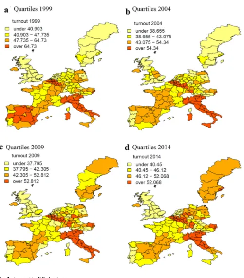
Figure 1 shows the quartiles of turnout in the 1999, 2004, 2009, and 2014 elec-tions across 155 European regions respectively. The figure significantly denotes changes in the countries’ and regions’ level of turnout during the four considered EP elections. It also shows that there are well-defined clusters of regions charac-terized by a high and low turnout respectively, indicating that regions that behave similarly are usually close to each other. Furthermore, large evidence supports the existence of economic interdependence among (cross-border) neighboring Euro-pean regions, as well as the presence of spillover effects across national borders (see Ertur et al. 2006). Recall that socio-economic factors are important contex-tual drivers of voter turnout (defined at regional level). All these arguments sug-gest that a more complete discussion of the determinants of voter turnout in the EP elections requires exploring spillover effects on turnout in bordering regions.
The paper is organized as follows: Sect. 2 describes the spatial features of turn-out. Section 3 introduces the model specification and the data, Sect. 4 presents the results and provides a discussion. Conclusions are drawn in Sect. 5.
2 Spatial properties of turnout
To analyze space dependence, the best-known indicator is Moran’s I (MI) (Moran
1950). MI relates the value of a given variable to the values of the same variable in neighboring areas, namely its spatial lag. The intuition is that socio-economic phenomena might not be isolated in space and what is happening in a certain loca-tion may be correlated to what is happening in neighboring localoca-tions. We based the calculation of this measure of spatial autocorrelation on a row standardized queen spatial weight matrix W, where islands are connected to the closest region. Queen contiguity scheme makes a region to be connected to other regions if they touch for at least one point of the border, avoiding dropping neighboring relationships for regions even from two different countries. This allows for spatial spillovers across
regions belonging to the same and/or different countries. When the spatial matrix standardized by row, the MI varies between − 1 and 1. A positive coefficient points to positive spatial autocorrelation, i.e. clusters of similar values can be identified. The reverse represents regimes with negative associations, i.e. dissimilar values clustered together in a map. A value close to zero indicates a random spatial pattern.
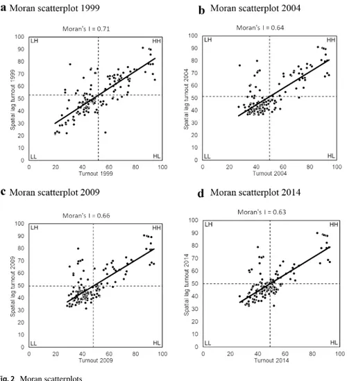
One advantage of this statistic is that it can be visualized in a so-called Moran scatterplot, with the spatial lag of the (standardized) variable on the vertical axis and the original (standardized) variable on the horizontal axis. Thus, each point in the scatterplot represents a combination of a location’s value and its correspond-ing values in the surroundcorrespond-ing regions, i.e. the spatial lag. The x- and y-axes divide the scatterplot into 4 quadrants (anticlockwise from top right): in the first and third (high–high, HH, and low–low, LL, respectively) a location that exhibits a high (low) value of the variable is surrounded by locations also with a high (low) value for the variable. In the second and fourth (low–high, LH, and high-low, HL, respectively) a location with a low (high) value of the variable is surrounded by locations with a high (low) value for the variable. A concentration of points in the first and third quadrants means positive spatial dependence (nearby locations have similar val-ues), while the concentration of points in the second and fourth quadrants reveals the presence of negative spatial dependence (i.e. nearby locations have dissimilar values).
The Moran scatterplots (Fig. 2) based on a queen row standardized spatial weight matrix show positive slopes and the concentration of points representing the regions in the first and third quadrant suggests that areas with high (low) turnout are clus-tered in space. In our case, at the top of the Moran scatterplot, MI is shown and is quite stable above 0.60. This means that there is spatial persistence over time, with well-defined clusters of regions characterized by high and low turnout, respectively.
Nevertheless, a closer look at the points in the Moran scatterplots reveals that their distribution is much more widespread in 1999 than in 2014, with a group of Belgian regions steadily located in the upper part of the first quadrant.1 Despite the fairly stable value of MI, this indicates a changing pattern in EU turnout. Such a pat-tern, without altering the ranking of EU regions in terms of turnout, signals greater similarity over time.
3 Model specification, variables and methodology
The analysis includes 12 EU countries (Portugal, Spain, France, Belgium, Luxem-bourg, the Netherlands, UK, Germany, Italy, Greece, Austria, and Sweden) for 155 regions.2 The data for turnout is from the European Election Database and national sources regarding four elections: 1999, 2004, 2009, and 2014.
1 We have to bear in mind in Belgium voting is compulsory.
2 For the method used, balanced panel data are essential. Greece is analyzed as a single region because
of the lack of data for 2014. In the other cases, we refer to NUTS-2 regions with the exception of the UK, Spain and Germany where NUTS-1 regions are used. Despite differences in size and administrative importance, it is common practice to consider these regions together. Finland has been excluded because regional data are only available for 1999 and 2004.
The time dimension of the data is used via a panel structure. In addition, we assume that the turnout in EP elections is affected by several regional and national factors, including the average level of turnout in the neighboring regions, and we estimate the following regression:
where Turnout is a n × 1 vector of the dependent variable, that is the number of votes on registered citizens in each region at election year t. t is the election year (1999, 2004, 2009, 2014) and ut the i.i.d. residuals. W is the n × n Queen spatial matrix, and
Wt is a space–time spatial weight matrix defined as It⊗ W where ⊗ represents the
Kronecker product and It the identity matrix of size t. The n × 1 vector WtTurnout
(1)
Turnoutt= a0+ 𝜌𝐖tTurnoutt+ a2𝐒𝐎𝐂𝐄𝐂t+ a3𝐏𝐎𝐋𝐈𝐍𝐒𝐓t+ At+ ut
defines the spatially weighted linear combination of the turnout in neighboring regions, and the coefficient ρ measures the strength of the relation between turn-out in a region (the dependent variable) and the neighbors.3 Following Gimpel et al. (2004), we estimate pooled data from the four election years, including dummy vari-ables At for each year (using 1999 as the baseline). Equation (1) is estimated with a standard maximum likelihood approach (ML) (Anselin 1988) and with a heter-oskedastic-consistent ML (Cribari-Neto 2004). Furthermore, we perform robustness using alternative methods that account for the endogeneity of the spatial autoregres-sive coefficient, namely two-stage least squares (S2SLS) and spatial two-stage least squares with a heteroskedasticity and autocorrelation-consistent (HAC) estimator of the variance–covariance matrix (S2SLSHAC), as well as through generalized spatial two-stage least squares (GS2SLS) (Kelejian and Prucha 1999). Finally, we estimate the model with generalized spatial two-stage least squares accounting for heteroske-dasticity in the error term (GS2SLSHET), using spatial lags of exogenous variables as instruments (Kelejian and Prucha 2010). Following Anselin and Rey (1991), the choice of the spatial lag model is performed through a Lagrange Multiplier (LM) test on OLS estimates to choose the spatial model (Anselin and Rey 1991).4
The vector SOCEC includes several regional economic as well as socio-eco-nomic variables at the aggregate level.5 GDP per capita (the logarithm for GDP per capita in PPS, source of data Eurostat Regional Database)6 is the usual indicator of economic development (Shachar and Nalebuff 1999), Unemployment measures the percentage of long-term unemployed in total unemployment (source: Eurostat Regional Database) to control for labor market conditions (Verba et al. 1995; Rosen-stone 1982). The vector also includes Density (the log of the number of inhabitants per km2, source Eurostat Regional Database for population and Cambridge Econo-metrics for regional areas) (Oliver 2000) and the Dependency ratio (the percentage of people aged over 65 years and youngsters between 20 and 24, source Eurostat Regio Database) (Franklin and Holbot 2011). Participation in EP elections, and more generally attitudes towards the EU, may be based on the experiences of voters with the EU, for example, through funds that they receive from Bruxelles.
Objec-tive 1 regions is a dummy variable equal to 1 if regions are below 75% of EU GDP
per capita and thus receive the majority of EU Structural Funds, and 0 otherwise
4 According to the decision rule (Anselin et al. 1996), if the LM lag is more significant than the LM
error, and the robust LM lag is significant but the robust LM error is not, then the appropriate model is the spatial lag model. Conversely, if the LM error is more significant than the LM lag, and the robust LM error is significant but the robust LM lag is not, then the appropriate model is the spatial error model.
5 When using aggregate-level data inference may suffer from aggregation bias. However, this problem is
far less severe with regional-level data (see Kim et al. 2003).
6 Due to lack of data, the following years are used: 2000, 2004, 2009 and 2013.
3 As for the estimation of the Moran’s, the matrix W is a queen row standardized spatial weight matrix,
where islands are connected to the closest region. Results are robust to different neighbor definitions. As
(Mattila 2003, Flickinger and Studlar 2007; Fiorino et al. 2019).7 Finally, the vari-able Education measures the share of people aged 15–64 with upper secondary and post-secondary non-tertiary education (source: Eurostat Regio Database, lev-els 3 and 4). Multiple explanations have been proposed to explain the link between education and turnout. Among other effects, education impacts the vote because it enhances political interest and political knowledge, encourages the sense of civic responsibility and increases political efficacy (among others, Nie et al. 1996; Gal-lego 2010).
The vector POLINST includes a set of politico-institutional variables.
Institu-tional quality captures at the regional level good governance, that is high
impartial-ity and qualimpartial-ity of public service delivery, along with low corruption (source of data for 2014 is Teorell et al. 2020 and for 1999, 2004 and 2009 is Crescenzi et al. 2016). A perception of bad quality of political and institutional systems may compromise citizens’ satisfaction, lower generalized trust and lead many individuals to abstain from elections (Rothstein and Teorell 2008; Sundstrom and Stockemer 2015).
Her-findahl gov and HerHer-findahl opp measure respectively the sum of the squared seat
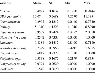
shares of all government or opposition parties. These variables are meant to cap-ture the fractionalization of the government and the opposition, respectively. They are defined at the national level (source: Beck et al. 2001). Compulsory voting and Week vote are linked to the national electoral systems and have largely been explored in the literature (among others, Franklin 2002). While compulsory voting leads to higher turnout rates, elections on weekdays decrease electoral participation since people follow their daily routines. The sources of both these variables are the national electoral agencies. Table 1 reports the descriptive statistics.
Table 1 Descriptive statistics Variable Mean SD Min. Max.
Turnout 0.4997 0.1637 0.1960 0.9444 GDP per capita 10.084 0.2688 9.2670 11.135 Unemployment 0.3902 0.1312 0.0410 0.7540 Density 5.1310 1.1328 1.1940 8.8990 Dependency ratio 0.9537 0.2424 0.3952 2.0510 Objective 1 regions 0.2542 0.4305 0.0000 1.0000 Education 0.4384 0.1412 0.8400 0.7180 Institutional quality 0.7379 0.3956 − 2.4210 1.6365 Herfindahl gov. 0.6817 0.2328 0.1810 1.0000 Herfindahl opp. 0.5838 0.1672 0.2199 0.8554 Compulsory voting 0.0774 0.2620 0.0000 1.0000 Week vote 0.1548 0.3620 0.0000 1.0000
7 This dummy variable is based on information available online (see http://ec.europ a.eu/regio nal_polic y/
Table
2
Linear spatial lag model r
esults OL S (1) ML (2) Robus t ML (3) S2SL S (4) S2SL SHA C (5) GS2SL S (6) GS2SL SHET (7) Int er cep t − 0.2559 − 0.3213 − 0.3213 − 0.3213 − 0.3213 − 0.3212 − 0.3212 (0.2048) (0.2026) (0.2077) (0.2025) (0.2136) (0.2025) (0.2152) GDP per capit a 0.0586*** 0.0602*** 0.0602*** 0.0600*** 0.0600*** 0.0605*** 0.0605*** (0.0207) (0.0203) (0.0205) (0.0206) (0.0207) (0.0207) (0.0208) U nem plo yment 0.1196*** 0.1160*** 0.1160** 0.1163*** 0.1163** 0.1150*** 0.1150** (0.0424) (0.0415) (0.0459) (0.0421) (0.0460) (0.0422) (0.0461) Density 0.0032 0.0018 0.0018 0.0019 0.0019 0.0019 0.0019 (0.0049) (0.0048) (0.0049) (0.0049) (0.0049) (0.0049) (0.0049) Dependency r atio 0.1026*** 0.0997*** 0.0997*** 0.0999*** 0.0999*** 0.1002*** 0.1002*** (0.0201) (0.0197) (0.0212) (0.0199) (0.0212) (0.0200) (0.0213) Education − 0.0442 − 0.0334 − 0.0334 − 0.0341 − 0.0341 − 0.0339 − 0.0339 (0.0354) (0.0349) (0.0381) (0.0354) (0.0385) (0.0357) (0.0387) Ins titutional q uality 0.0243** 0.0258** 0.0258*** 0.0257** 0.0257*** 0.0260** 0.0260*** (0.0121) (0.0119) (0.0094) (0.0120) (0.0094) (0.0120) (0.0093) Objectiv e 1 r egions − 0.0221** − 0.0215** − 0.0215** − 0.0216** − 0.0216** − 0.0213** − 0.0213** (0.0093) (0.0091) (0.0091) (0.0092) (0.0091) (0.0093) (0.0091) Herfindahl go v. − 0.0541** − 0.0496** − 0.0496* − 0.0499** − 0.0499* − 0.0486* − 0.0486* (0.0254) (0.0239) (0.0277) (0.0253) (0.0279) (0.0254) (0.0281) Herfindahl opp. 0.3660*** 0.3652*** 0.3652*** 0.3652*** 0.3652*** 0.3647*** 0.3647*** (0.0339) (0.0332) (0.0361) (0.0337) (0.0361) (0.0337) (0.0362) Com pulsor y v oting 0.4668*** 0.4569*** 0.4569*** 0.4575*** 0.4575*** 0.4595*** 0.4595*** (0.0199) (0.0199) (0.0167) (0.0202) (0.0172) (0.0203) (0.0173) W eek v ot e − 0.0898*** − 0.0806*** − 0.0806*** − 0.0812*** − 0.0812*** − 0.0812*** − 0.0812*** (0.0121) (0.0121) (0.0121) (0.0126) (0.0123) (0.0128) (0.0124) Tur nout in t he neighbor s 0.0851*** 0.0851*** 0.0888** 0.0888** 0.0868** 0.0868**
Table 2 (continued) OL S (1) ML (2) Robus t ML (3) S2SL S (4) S2SL SHA C (5) GS2SL S (6) GS2SL SHET (7) (0.0321) (0.0321) (0.0395) (0.0350) (0.0397) (0.0350) Time dummies Ye s Ye s Ye s Ye s Ye s Ye s Ye s Lambda − 0.0323 R^2 0.7085 0.7126 AIC − 1217.8 − 1224.6 Br eush P ag an tes t 95.205 *** 93.865*** LM er ror 5.6709** LM lag 9.0170 *** Robus t LM er ror 0.5573 Robus t LM lag 3.9034**
Significant at 1%, **significant at 5%, ***significant at 10%. In br
ac ke ts p v alues. R obus t LM s td. er rors es timated f ollo wing Cr ibar i-N eto ( 2004 ). LR tes t is com puted t o es timate t he significance of t he Tur nout in t he neighbor s f or ML and R obus t ML es timates
4 Results and discussion
Our results are displayed in Table 2, with the OLS regression. The LM tests for autocorrelation applied to the OLS residuals clearly show that spatial dependence in the form of spatial lag is present in the residuals. The Akaike Information Criterion (AIC) performed on the spatial lag ML model and OLS confirms the choice of the former, whose AIC is equal to − 643.59 against the − 582.24 of OLS.
When the spatial structure is included in the model, the value of the depend-ent variable in one spatial unit is affected by the independdepend-ent variables in nearby units. In this case, the assumption of uncorrelated error terms as well as inde-pendent observations is violated. As a result, parameter estimates are biased and inefficient. Furthermore, as shown by the Breush Pagan test, the presence of het-eroscedasticity in the OLS and spatial lag models is a source of additional ineffi-ciency in the standard error estimation. This calls for the estimation of heteroske-dastic robust models, in columns 3, 5, and 7.
However, the spatial lag models estimated using different estimators show con-sistent results, highlighting the robustness of our specification even when heter-oskedasticity is accounted for. Although the standard errors increase, overall, the statistical significance of the parameters does not change.
The presence of a positive significant spatial autoregressive parameter ρ signals the existence of global externalities due to how the spatial multiplier is defined, i.e. as (I − Wρ)−1 = I + Wρ + W2ρ2+ ··· + WNρN, where I is an N × N the identity matrix.
Thus, turnout is determined by each region’s own factors as well as those of imme-diate neighbors (ρW), second-order neighbors (W2ρ2) and so forth.
Indeed, a shock in region i is transmitted to its neighbors by parameter ρ related to turnout in neighbors and, in turn, this is transmitted back to region i through 𝐖 , reinitiating the process until the effect becomes negligible for N tend-ing towards infinity (LeSage and Fischer 2008).
The spatial autoregressive parameter is comprised between 0.0851 and 0.0888 corresponding, in scalar terms, to a spatial multiplier around 1.09. This implies that around 90% of turnout is explained by direct effects, i.e. the impact of a change in a variable in the same region i, while the remainder, the so-called indirect or spillo-ver effect, is given by the effect arising from changes in a variable in the neighbors. Note that in an OLS ρ = 0 thus, if there is spatial dependence in the dependent vari-able, the regression coefficients are upward biased. We argue that one of the possible sources of spillover effects might be commuting (LeSage and Dominguez 2012).
We discuss the results for regional variables when we comment direct, indirect and total effects. Here we comment on the national variables. Compulsory voting has the expected positive effect on turnout, whereas Week vote has the expected negative effect since voting becomes more costly. In both cases, the coefficients are very consistent and significant at the highest level. The fractionalization of the government and opposition have opposite effects on turnout. The significance of the former is smaller than for the latter.
Direct, indirect and total effects for the regional variables are shown in Table 3
to offer a richer interpretation of our results in terms of spillover effects. Indeed, change in a single observation (region) associated with each explanatory variable may affect the region itself (direct effect) and potentially all the other regions indirectly (an indirect effect) (LeSage and Pace 2009). The positive and sig-nificant GDP per capita suggests that an improvement in economic conditions promotes the political engagement of citizens (Radcliff 1992). This is valid for a change in the region of study, but also if a shock occurs in the neighborhood because of social and economic interconnections between regions.8 Dissatisfac-tion in labor market condiDissatisfac-tions is a salient issue to be relevant for the decision of whether to vote or not. The results show that Unemployment is positively related to voting in EP elections, which provides evidence in favor of the mobilization approach (Rosenstone 1982).
The Dependency ratio is also positively correlated with the turnout: the oldest segment of the population is more likely to vote than the youngest. This confirms that the age structure of the population helps to explain variations in the electoral behavior of voters.
Objective 1 regions have significantly negative coefficients. Although
margin-alized areas receive funds from the EU, they appear less interested in European
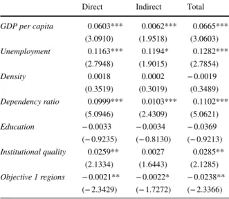
Table 3 Estimates of direct, indirect and total effects based on the estimates of ML models in Table 2
Significant at 1%, **significant at 5%, ***significant at 10%. In brackets, direct, indirect, and total effects and related t-statistics computed using 1000 draws from the estimated variance–covariance matrix of parameters (the spatial multiplier (I− ρW)−1 is calculated
every draw
Direct Indirect Total
GDP per capita 0.0603*** 0.0062*** 0.0665*** (3.0910) (1.9518) (3.0603) Unemployment 0.1163*** 0.1194* 0.1282*** (2.7948) (1.9015) (2.7854) Density 0.0018 0.0002 − 0.0019 (0.3519) (0.3019) (0.3489) Dependency ratio 0.0999*** 0.0103*** 0.1102*** (5.0946) (2.4309) (5.0621) Education − 0.0033 − 0.0034 − 0.0369 (− 0.9235) (− 0.8130) (− 0.9213) Institutional quality 0.0259** 0.0027 0.0285** (2.1334) (1.6443) (2.1285) Objective 1 regions − 0.0021** − 0.0022* − 0.0238** (− 2.3429) (− 1.7272) (− 2.3366)
8 Note that the estimated coefficients and the direct effects do not match perfectly. The difference is due
to the positive feedback effect arising from impacts passing through neighboring regions and back to the region itself, given by the W matrix.
politics than in other areas. The responsiveness and effectiveness of institutions at the regional level enhances the willingness of people to engage in voting.
There is no significant relationship between population density and turnout. The often-found results that in relatively low-density areas relationships are closer and lead to ‘social pressure’ to vote (Overbye 1995) are possibly undone by the per-ceived distance of the EP. Also Education does not impact voter turnout, a result that is not new among previous studies on European democracies (among others, Lijphart 1997; Norris 2002; Teorell, et al. 2007), but that is at odds with several works on political behavior (e.g., Burden 2009; Gallego 2010).
5 Conclusions
This paper analyzes the geographical features of voter turnout in the four EP elec-tions held from 1999 to 2014 in 155 European regions. We find some spillover effects that are presumably due to commuting, cultural traits, and values that neigh-boring communities share. Our results point out how changes in some determinants in a region influence voter turnout in the same region (direct effects) as well as turn-out in the neighboring ones (indirect effects), indicating that there may be additional benefits to turnout that spill-over the border of a region. Indirect effects are smaller than direct effects, but failing to account for them results in a partial understanding of the interrelation between dependent variables and turnout.
Funding Open Access funding provided by Università degli Studi di Verona.
Open Access This article is licensed under a Creative Commons Attribution 4.0 International License, which permits use, sharing, adaptation, distribution and reproduction in any medium or format, as long as you give appropriate credit to the original author(s) and the source, provide a link to the Creative Com-mons licence, and indicate if changes were made. The images or other third party material in this article are included in the article’s Creative Commons licence, unless indicated otherwise in a credit line to the material. If material is not included in the article’s Creative Commons licence and your intended use is not permitted by statutory regulation or exceeds the permitted use, you will need to obtain permission directly from the copyright holder. To view a copy of this licence, visit http://creat iveco mmons .org/licen ses/by/4.0/.
References
Agnew, J.: Place and Politics: The Geographical Mediation of State and Society. Allen and Unwin, Bos-ton (1987)
Anselin, L.: Spatial Econometrics: Methods and Models. Kluwer Academic Publishers, Dordrecht (1988) Anselin, L., Rey, S.: Properties of tests for spatial dependence in linear regression models. Geogr. Anal.
23, 112–131 (1991)
Anselin, L., Bera, A., Florax, R., Yoon, M.: Simple diagnostic tests for spatial dependence. Reg. Sci. Urban Econ. 26, 77–104 (1996)
Beck, T., Clarke, G., Groff, A., Keefer, P., Walsh, P.: New tools in comparative political economy: the Database of Political Institutions. World Bank Econ. Rev. 15, 165–176 (2001)
Books, J.W., Prysby, C.L.: Political Behavior and the Local Context. Praeger, New York (1991) Burden, B.C.: The dynamic effects of education on voter turnout. Electoral. Stud. 28, 540–549 (2009) Cancela, J., Geys, B.: Explaining voter turnout: a meta-analysis of national and subnational elections.
Electoral. Stud. 42, 264–275 (2016)
Crescenzi, R., Rodriguez-, Pose A., Di Cataldo, M.: Government quality and the economic returns of transport infrastructure investment in European regions. J. Reg. Sci. 56, 555–582 (2016)
Cribari-Neto, F.: Asymptotic inference under heteroskedasticity of unknown form. Comput. Stat. Data Anal. 45, 215–233 (2004)
Ertur, C., Le Gallo, J., Baumont, C.: The European regional convergence process, 1980–1995: do spatial regimes and spatial dependence matter? Int. Reg. Sci. Rev. 29, 3–34 (2006)
Fiorino, N., Pontarollo, N., Ricciuti, R.: Supra national, national and regional dimensions of voter turnout in European parliament elections. J. Common Mark. Stud. 57, 877–893 (2019)
Flickinger, R.S., Studlar, D.T.: One Europe, many electorates? models of turnout in European parliament elections after 2004. Comp. Polit. Stud. 40, 383–404 (2007)
Foley, P., Demšar, U.: Using geo-visual analytics to compare the performance of Geographically Weighted Discriminant Analysis versus its global counterpart, Linear Discriminant Analysis. Int. J. Geogr. Inf. Sci. 27, 633–661 (2013)
Franklin, M.: Electoral participation. In: Leduc, L., et al. (eds.) Comparing Democracies: New Chal-lenges in the Study of Elections and Voting, pp. 148–168. Sage, London (2002)
Franklin, M., Holbot, S.: The legacy of lethargy: how elections to the european parliament depress turn-out. Electoral. Stud. 30, 67–76 (2011)
Gallego, A.: Understanding unequal turnout: education and voting in comparative perspective. Electoral. Stud. 29, 239–248 (2010)
Gimpel, G.J., Morris, I.L., Armstrong, D.R.: Turnout and the local age distribution: examining political participation across space and time. Polit. Geogr. 23, 71–95 (2004)
Holbot, S.B.: Citizen satisfaction with democracy in the European union. J. Common Mark. Stud. 50, 88–105 (2012)
Huckfeldt, R., Sprague, J.: Citizens, Politics and Social Communication: Information and Influence in an Election Campaign. Cambridge University Press, Cambridge (1995)
Kelejian, H., Prucha, I.: A generalized moments estimator for the autoregressive parameter in a spatial model. Int. Econ. Rev. 40, 509–533 (1999)
Kelejian, H., Prucha, I.: Specification and estimation of spatial autoregressive models with autoregressive and heteroscedastic disturbances. J. Econom. 157, 53–67 (2010)
Kim, J., Elliot, E., Wang, D.M.: A spatial analysis of country-level outcomes in U.S. Presidential Elec-tions. Elect. Stud. 22, 741–761 (2003)
Lacombe, D.J., Holloway, G.J., Shaughnessy, T.M.: Bayesian estimation of the spatial durbin error model with an application to voter turnout in the 2004 presidential election. Int. Reg. Sci. Rev. 37, 298–327 (2014)
LeSage, J.P., Dominguez, M.: The importance of modeling spatial spillovers in public choice analysis. Public Choice 150, 525–545 (2012)
LeSage, J.P., Fischer, M.M.: Spatial growth regressions: model specification, estimation and interpreta-tion. Spat. Econ. Anal 3, 275–304 (2008)
LeSage, J.P., Pace, R.K.: Introduction to Spatial Econometrics. Taylor & Francis CRC Press, Boca Raton (2009)
Lijphart, A.: Unequal participation: democracy’s unresolved dilemma. Am. Polit. Sci. Rev. 91, 1–14 (1997)
Mansley, E., Demšar, U.: Space matters: geographic variability of electoral turnout determinants in the 2012 London mayoral election. Elect. Stud. 40, 322–334 (2015)
Mattila, M.: Why bother? determinants of turnout in the European elections. Elect. Stud. 22, 449–468 (2003)
Moran, P.A.P.: Notes on continuous stochastic phenomena. Biometrika 37, 17–23 (1950)
Nie, N.H., Junn, J., Stehlik-Barry, K.: Education and Democratic Citizenship in America. University of Chicago Press, Chicago (1996)
Norris, P.: Democratic Phoenix: Reinventing Political Activism. Cambridge University Press, Cambridge (2002)
Oliver, J.E.: City size and civic involvement in Metropolitan America. Am. Polit. Sci. Rev. 94, 361–373 (2000)
Overbye, E.: Making a case for the rational, self-regarding ‘ethical’ voter and solving the ‘paradox of not voting’ in the process. Eur. J. Polit. Res. 27, 269–296 (1995)
Pattie, C.J., Johnston, R.J.: ‘People who talk together vote together’: an exploration of contextual effects in Great Britain. Ann. Assoc. Am. Geogr. 90, 41–66 (2000)
Pattie, C.J., Johnston, R.J.: It’s not like that round here: region, economic evaluations and voting at the 1992 British General Election. Eur. J. Polit. Res. 28, 1–32 (1995)
Radcliff, B.: The welfare state, turnout, and the economy: a comparative analysis. Am. Polit. Sci. Rev. 86, 444–454 (1992)
Rothstein, B., Teorell, J.: What is quality of government? A theory of impartial political institutions. Int. J. Policy Adm. 21, 165–190 (2008)
Rosenstone, S.: Economic adversity and voter turnout. Am. J. Polit. Sci. 26(1), 25–46 (1982)
Shachar, R., Nalebuff, B.: Follow the leader: theory and evidence on political participation. Am. Econ. Rev. 89, 525–547 (1999)
Shin, M., Agnew, J.A.: Spatial regression for electoral studies: the case of the Italian Lega Nord. In: Warf, B., Lieb, J. (eds.) Revitalizing Electoral Geography, pp. 59–74. Ashgate, Farnham (2011) Smets, K., van Ham, C.: The embarrassment of riches? a meta-analysis of individual-level research on
voter turnout. Elect. Stud. 32, 344–359 (2013)
Sundstrom, A., Stockemer, D.: Regional variation in voter turnout in Europe: the impact of corruption perceptions. Elect. Stud. 40, 158–169 (2015)
Tam Cho, W.K., Rudolph, T.J.: Emanating political participation: untangling the spatial structure behind participation. Br. J. Polit. Sci. 38, 273–289 (2008)
Teorell, J., Dahlberg, S., Holmberg, S., Rothstein, B., Alvarado Pachon, N., Axelsson, S.: The Quality of Government Standard Dataset, version Jan20. University of Gothenburg, The Quality of Govern-ment Institute (2020)
Teorell, J., Sum, P., Tobiasen, M.: Participation and political equality: an assessment of large-scale democracy. In: van Deth, J., Montero, J.R., Westholm, A. (eds.) Citizenship and Involvement in European Democracies: A Comparative Perspective, pp. 384–414. Routledge, London (2007) Verba, S., Schlozman, K.L., Henry, E., Brady, H.E.: Voice and Equality: Civic Voluntarism in American
Politics. Harvard University Press, Cambridge (1995)
Wing, S.I., Walker, J.L.: The geographic dimensions of electoral polarization in the 2004 U.S. Presiden-tial vote. In: Paez, A., Le Gallo, J., Buliung, R., Dall’Erba, S. (eds.) Progress in SpaPresiden-tial Analysis: Theory and Computation, and Thematic Applications, pp. 253–285. Springer, Berlin (2010)
Publisher’s Note Springer Nature remains neutral with regard to jurisdictional claims in published maps and institutional affiliations.