Fault delineation and stress orientations from the analysis of background, low magnitude seismicity in Southern Apennines (Italy)

(1)

UNIVERSITÀ DI BOLOGNA ―ALMA MATER STUDIORUM‖

D

OTTORATO DI

R

ICERCA IN

G

EOFISICA

XXIV

CICLO

Settore concorsuale 04/04

Settore scientifico disciplinare GEO/10

Fault delineation and stress orientations

from the analysis of background, low

magnitude seismicity in Southern

Apennines (Italy)

Tesi di dottorato

Emanuela Matrullo

Tutore Coordinatore

Prof. R. De Matteis Prof. M. Dragoni

Supervisore

Dott. A. Emolo

(2)

(3)

3

Fault delineation and stress orientations from the analysis of background, low magnitude seismicity in Southern Apennines (Italy)

“You've got to find what you love. And that is as true for your work as it is for your lovers. Your work is going to fill a large part of your life, and the only way

to be truly satisfied is to do what you believe is great work. And the only way to do great work is to love what you do. If you haven't found it yet, keep looking. Don't settle. As with all matters of the heart, you'll know when you find it. And, like any great relationship, it just gets better and better as the years roll on. So keep looking until you find it.

Don't settle.…Stay Hungry. Stay Foolish....” Steve Jobs

(4)

(5)

5

Table of Contents

Introduction

In active seismic regions knowing the precise location, geometry and character of fault structures is of great interest for studies of tectonic processes, ongoing Earth‘s deformation, and hazard assessment. One important issue is whether the background, low magnitude seismicity allows to identify the faults causative of moderate to large earthquakes and to infer information about the present stress field acting in the area. The main limitations of using micro-seismicity to study active faults generally derive from the relatively large hypocentral errors due to network geometry, number and accuracy of arrival time readings, the inaccuracy of the crustal velocity model but also from the possible uncorrelation of microearthquake occurrence with faults and regional stress regime responsible of large earthquakes. Thanks to the development of regional dense seismic networks, it is possible nowadays to have high quality recordings of small earthquakes that can be used to highly improve the accuracy in location, focal mechanism and stress field estimation, so that their relationship with major faults can be quantitatively assessed. Several studies worldwide have shown that high precision earthquake locations produce sharpening of seismicity patterns allowing to determine the fine-scale fault geometry and extent (Rubin et al., 1999; Waldhauser and Ellsworth, 2000; Hauksson and Shearer, 2005; Lin et al., 2007). Most of these studies concern the seismicity of California, a region characterized by a dominant strike-slip tectonics, suitable for the identification of streaks of microearthquakes along active fault surfaces. Only few microseismicity studies performed in normal/thrust tectonic stress environments show a robust correlation between the background low magnitude seismicity and location and geometry of active faults causative of large earthquakes (Evans et al., 1985; Suarez et al., 1990; Rigo et al., 1996). This is specifically the case of the Apenninic chain in Italy, where the background microseismicity, recorded by the permanent National Seismic Network of the Istituto Nazionale di Geofisica e Vulcanologia (INGV), shows a quite diffused

(8)

pattern of locations, spread across the axis chain, with a poor correlation with existing and known fault structures. On the other hand, several examples exist, showing that the locations of aftershocks recorded immediately after a moderate to large event accurately delineate the geometry of the fault planes and can be used to estimate the stress field thanks to the high quality of data and the improved techniques of analysis (e.g. Chiaraluce et al., 2003).

The goal of this thesis is to show that refined analyses of background, low magnitude seismicity in the dominant normal-faulting tectonic region of Southern Apennines allow to delineate the main active faults and to accurately estimate the directions of the regional tectonic stress. This region is among the areas of Italy with the highest seismic potential and it has been the target of a project of a prototype system for Earthquake Early Warning (Zollo et al., 2009). Moreover this area is characterized by complex geological-structural architecture. This complexity is related to the deformation of three main paleogeographic domains: the Lagonegro Basin located between the Western Carbonate and Apulia Carbonate Platforms. The tectonics of this area is accommodated by the collision between the Adriatic micro-plate and the Apenninic belt, derived by the convergence between the Euro-Asian and African plates. The eastward migration of the thrust-belt–foredeep–foreland system caused by the west-dipping subduction process of the Adriatic microplate is related to the opening of the Tyrrhenian basin (Patacca et al., 1990). The background seismicity is mainly distributed along the axis of the Apenninic chain and it is characterized by low to moderate magnitude earthquakes (M < 3). The most recent destructive earthquake occurred in the Irpinia region on November 23, 1980, M 6.9 and has been studied in detail by many authors using different geophysical data sets (Westaway and Jackson, 1987; Bernard and Zollo, 1989; Pantosti and Valensise, 1990). The 1980 earthquake was a pure normal faulting event; it occurred on approximately 60 Km long, NW-SE striking, fault segments with three main rupture episodes at 10, 18 and 39 s from the first shock. Since 1980, the largest event that occurred within the epicentral area of the

(9)

9

Introduction

1980 earthquake was the April 3, 1996 earthquake (ML=4.9), also characterized

by a normal faulting mechanism (Cocco et al., 1999). Two moderate magnitude seismic sequences occurred between 1990 and 1991 in the Potenza region located about 40 Km SE of the 1980 Irpinia aftershock area (Ekstrom, et al., 1994). The two mainshocks (ML=5.2 and ML=4.7) and the larger events of the sequences

were characterized by strike-slip faulting mechanisms with preferred fault planes having an E-W orientation (Di Luccio et al., 2005).

The low magnitude earthquake data (0.1 <ML< 3.2) analyzed in this work have

been acquired by the National Seismic Network and the Irpinia Seismic Network (ISNet), a dense and wide dynamic network deployed around and over the active fault system affecting the region and managed by the permanent research enterprise AMRA - Analysis and Monitoring of Environmental Risk.

The availability of high quality data-set has allowed us to perform several analyses to characterize the area from a seismological point of view and to increase the details of the knowledge about this complex crustal structure. We want to underline here the innovation of the contribution obtained from the analysis of background micro-seismicity in studies of active tectonics. This gives a new perspective to the application of the high quality records of background seismicity for the identification and characterization of active fault systems, which can integrate the information provided by low magnitude seismicity about the active stress regime.

Taking into account the peculiarities of the investigated area and of the tectonic environment, different methods must be adopted in order to better define the fault structures.

The definition of the fault structures requires accurate localization and it cannot be exempt from the correct understanding of the propagation medium. This is important to reduce uncertainties and distortion in the position of hypocenters that may result in artifacts such as apparent lineations (Michelini and Lomax, 2004). Three-dimensional (3D) features of the propagation medium are generally

(10)

unknown, and so simplified one dimensional (1D) velocity models are generally used in the earthquakes location.

The known strong lateral variation of the elastic properties of the medium in the investigated area called into question the representativeness of the 1D velocity model and the role of the static station corrections for the earthquakes location. In this kind of studies it‘s important a detailed study for the velocity model determination and an accurate analysis on the effects that the use of 1D velocity models to represent the true three dimensional velocity distribution induces on earthquake locations. The effects of an unsuitable velocity model on hypocenter locations can be minimized by using relative earthquake location methods (Frèchet, 1985; Got et al., 1994). An additional improvement in the location precision can be also obtained by improving the accuracy of the relative arrival-time readings using waveform cross-correlation methods (Waldhauser, 2002). These features make it possible to obtain sharp streaks of microearthquakes especially for strike slip vertical faults as is the case examined in the region of Potenza. But an additional complexity in tectonic settings characterized by extensional regime is due to the presence of normal faults with a dip from 50° to 70°. And so the epicentral characteristics of the seismicity could not display linear trends as for near vertical faults. The study of the focal solutions can in these cases provide information on the presence of random or highly organized structures and can help to understand the orientation and the geometry of the fault planes.

In order to better understanding the geodynamic processes and interpret the seismicity and the fault systems from a seismtectonic point of view, it‘s important to define the stress field acting in the area. Several inversion techniques are used to determine the stress field and its possible spatial variations using earthquakes data. In particular the background seismicity and the aftershocks of a strong earthquake represent the only tools to study the state of stress acting in a region in depth. It‘s important to underline that the ability of the inversion to find an acceptable ―best‖ stress tensor is equally as important as

(11)

11

Introduction

to define meaningful errors on the stress directions. This is especially important if we are to look for spatial variations in the stress field, even in relatively small regions of space as the case examined.

The work carried out in the present research thesis is organized as follows.

The first chapter starts with a brief recall of the fundamental concepts of stress. We describe the different methodologies used to estimate the state of stress, including the use of fault data, information on borehole breakouts and focal mechanisms of earthquakes. In particular, we focus on the algorithm developed by Rivera L. and Cisternas A. (1990) that allows for the simultaneous estimation of the orientation and shape of the stress tensor and the individual fault plane solution given a population of earthquakes.

In the second chapter we describe the investigated area from a geological point of view. This is an important tool to understand the structural complexity of the analysed area, where the geological and geophysical knowledge reveal a significant lateral variation of the elastic properties of the medium along a direction perpendicular to Apenninic belt and characterized by a complex systems of faults with dominant normal-faulting tectonic.

In the third chapter we discuss about the creation and validation of seismological dataset recorded by ISNET and INGV networks. The presence in the studied area of an a hoc regional dense seismic network, allowed us to build a high quality recordings of small earthquakes and to obtain a dataset of very accurate arrival time readings and polarity of the P-wave first motion. This is important to improve the accuracy in location, velocity model, focal mechanism and stress field estimation.

In the fourth chapter we estimate a ―minimum‖ P-wave velocity model together with station corrections. We analyze the role of the station corrections and the effects on the earthquakes location in an area characterized by important lateral velocity variation. This study is supported by several synthetic tests and by the comparison with the location in a three dimensional model availed for the area.

(12)

The application of a methodology called Double Difference (DD; Waldhauser and Ellsworth, 2000) technique is used in order to improve the earthquake locations and permit to better delineate the fault systems.

In the first part of fifth chapter we illustrate the methodology behind the construction of the focal mechanism and compute the fault plane solutions for the selected earthquakes. In the second part we analyze the problem of the stress field determination using earthquakes data. A new method to compute the error on the stress field orientations will be implemented. We study the velocity models influence on the estimated parameters. The spatial variations of the stress field it will be investigated. The results of this analysis allow us to define the geometry of fault systems and to understand the geodynamic acting in the area. Finally, in the sixth chapter we propose our interpretation of the results presented in the previous chapters. An accurate discussion from a seismotectonic and geodynamic point of view concludes this work.

(13)

13

Chapter 1 Stress field determination

1.Introduction

The state of stress in the lithosphere is the result of the forces acting upon and within it. Knowledge of the magnitude and distribution of these forces can be combined with mechanical, thermal and rheological constraints to provide a better understanding of geodynamic and deformational processes (Bott, 1959; McKenzie, 1969). Stress makes geologic processes happen, and geologic processes make stress. Plate tectonics, glacial rebound, landslides, tidal deformation, phase changes, fluid flow, rock folding, and crystallization are example of processes that generate, modify, and consume stress within the Earth. Gravitational forces acting on and within the Earth are intimately connected to the stress state, and earthquakes occur when the shear stress exceeds the failure level for the fault.

In this section we want to analyze the state of stress in the brittle crust resulting from relatively large scale lithospheric process so that knowledge of crustal stress can be used to constrain the forces involved in these processes. Any quantitative description of seismic wave propagation or of earthquake physics requires the ability to characterize the internal forces between different parts of the medium, called stress. To better understand the nature and distribution of forces within the crust is essential to recall the fundamental concepts of the theory of stress, with particular reference to the determination of the principal axes of stress.

We briefly describe the different methodologies that allow us to obtain an estimate of the state of stress, including the use of fault data, information on borehole breakout and focal mechanisms of earthquakes. In particular we describe the algorithm developed by Rivera L. and Cisternas A. (1990) that

(14)

allows for the simultaneous estimation of orientation and shape of the stress tensor and the individual fault plane solution given a population of earthquakes from first P-motion polarities.

2. Aspects of stress tensor

Stress is a well-defined physical quantity throughout the interior of any fluid or solid material. Basic rules of force balance on a small material element lead to the construction of the stress tensor, which can be viewed as three mutually perpendicular force dipoles acting on the faces of the material element (Aki and Richards, 1980). These three dipoles are commonly referred to as principal stresses, and the units stress are force per unit area (1Pa = 1Nm-2_).

Figure 1.1 Stress tensor for a single vertical force dipole (zz) represented by isotropic and deviatoric components (a) or by Mohr‘s circle (b) (modified from Ruff, 2002).

The most important mathematically subdivision of the stress tensor is into the isotropic and deviatoric parts. As shown in Figure 1.1, isotropic part is formally defined as one-third the trace of the stress tensor; in other words pressure is the average value of the principal stresses.

Figure 1.1 also illustrates how a stress tensor for a single force dipole is decomposed into the isotropic part and deviatoric part.

A common description of the stress state is to quote the ―normal‖ and ―shear‖ stresses with respect to a particular plane slicing through the material. In this context normal stress refers to the force component acting perpendicular to the plane, whereas shear stress refers to the force component acting parallel to the plane. In the matrix representation of stress, normal and shear stresses are the

(15)

15

2.1 Stress tensor

diagonal and off-diagonal components of the stress tensor after it has been rotated to a new coordinate system that coincides with the plane orientation. Mohr‗s circles provide a clever geometric visualization of this view of the stress state (Figure 1.1) .

As a plane is rotated from an initial orientation that is normal to the maximum principal stress, then shear stress along the plane increases from its initial value of zero.

2.1 Stress tensor

In this paragraph, the theoretical treatment is from Shearer, (2009). Consider an infinitesimal plane of arbitrary orientation

within a homogeneous elastic medium in static equilibrium. The orientation of the plane may be specified by its unit normal vector, ̂. The force per unit

area exerted by the side in the direction of ̂ across this plane is termed the traction and is represented by the vector t( ̂) = (tx, ty, tz).

If t acts in the direction shown here, then the traction force is pulling the opposite side toward the interface. This definition is the usual convention in seismology and results in extensional forces being positive and compressional forces being negative. In some other fields, such as rock mechanics, the definition is reversed and compressional forces are positive. There is an equal and opposite force exerted by the side opposing ̂, such that t(− ̂) = −t( ̂). The part of t which is normal to the plane is known as normal stress, the one which is parallel is called shear stress. In case of a fluid, there are no shear stresses and t = −P ̂, where P is the pressure.

Figure 1.2 The traction vectors t( ̂ ),t( ̂ ), and t( ̂ ) describe the forces on the faces of an infinitesimal cube in a Cartesian coordinate system (from Shearer, 2009)

(16)

In general, the magnitude and direction of the traction vector will vary as a function of the orientation of the infinitesimal plane. Thus, to fully describe the internal forces in the medium, we need a general method for determining t as a function of ̂. This is accomplished with the stress tensor, which provides a linear mapping between ̂ and t.

The stress tensor, σ, in a Cartesian coordinate system (Figure 1.2) may be defined1_{by the tractions across the yz, xz, and xy planes:}

[ ( ̂) ( ̂) ( ̂) ( ̂) ( ̂) ( ̂) ( ̂) ( ̂) ( ̂) ] [ ] (1.1)

Since the solid is in static equilibrium, the equilibrium conditions reduces the number of independent parameters in the stress tensor to six, respect to nine that are present in the most general form of a second-order tensor.

[

] (1.2)

The traction across any arbitrary plane of orientation defined by ̂ may be obtained by multiplying the stress tensor by ̂, that is,

( ̂) ̂ [ ( ̂) ( ̂) ( ̂) ] [ ] [ ̂ ̂ ̂ ] (1.3) This can be shown by summing the forces on the surfaces of a tetrahedron (the

Cauchy tetrahedron) bounded by the plane normal to ̂ and the xy, xz, and yz

planes. The stress tensor is simply the linear operator that produces the traction vector t from the normal vector ̂, and, in this sense, the stress tensor exists independently of any particular coordinate system. For a practical purpose, we

(17)

17

2.1 Stress tensor

select a specific reference frame writing the stress tensor as a 3 × 3 matrix in a Cartesian geometry.

The stress tensor will normally vary with position in a material; it is a measure of the forces acting on infinitesimal planes at each point in the solid. Stress provides a measure only of the forces exerted across these planes. However, other forces may be present (e.g., gravity); these are denoted as body forces.

2.1.1Principal axes of stress

For a given state of stress, the traction vector acting on each surface within a material has components both normal and tangential to it. Since the stress tensor is real and symmetric, it is always possible to find a reference frame which makes it diagonal. The three axis defining this reference frame are called the principal stress axis. We can consider some surfaces specially oriented such that the shear tractions on them vanish. These surfaces can be characterized by their normal vectors, called principal stress axis; the normal stresses on this surface are called principal stresses. This concept is fundamental for the earthquake source mechanisms.

Thus, for any stress tensor, it is always possible to find a direction ̂ such that there are no shear stresses across the plane normal to ̂, that is, t( ̂) points in the ̂ direction. In this case

( ̂)= ̂ ̂

̂  ̂ (1.4) (  ) ̂

where I is the identity matrix and λ is a scalar multiplicative constant. This is an eigenvalue problem that has a non-trivial solution only when the determinant vanishes2_:

[  ] = 0 (1.5)

2_{A nontrivial solution exists only for values of}__{such that the matrix is singular (has no inverse),} which occurs when its determinant is zero

(18)

This is a cubic equation with always three solutions, the eigenvalues λ1, λ2, and λ3. Furthermore, since σ is symmetric and real, the eigenvalues are real. Corresponding to the eigenvalues are the eigenvectors ̂(1), ̂(2), and ̂(3). The eigenvectors are orthogonal and define the principal axes of stress. The planes perpendicular to these axes are termed the principal planes. We can rotate σ into the ̂(1), ̂(2), ̂(3) coordinate system by applying a similarity transformation

[ ] (1.6) Where σR _{is the rotated stress tensor and σ}₁_{, σ}₂_{, and σ}₃_{are the principal stresses}

(identical to the eigenvalues λ1, λ2, and λ3). Here N is the matrix of eigenvectors

[

( ) ( ) ( ) ( ) ( ) ( ) ( ) ( ) ( )

] (1.7)

By convention, the three principal stresses are sorted by size, such that |σ1| >|σ2| >|σ3|. The maximum shear stress occurs on planes at 45° to the maximum

and minimum principle stress axes. In the principal axes coordinate system, one of these planes has normal vector ̂= (1/√ , 0, 1/√ ). The traction vector for the stress across this plane is

( ) [ ] [ √ √

] [ √ √

] (1.8)

This can be decomposed into normal and shear stresses on the plane:

( )= ( ) ( √ √ ) ( ) (1.9) ( )= ( ) ( √ √ ) ( ) (1.10)

(19)

19

2.1 Stress tensor

and we see that the maximum shear stress is (σ1 − σ3)/2.

Figure 1.3 (modified from (Zoback et al., 2002) Definition of stress tensor in an arbitrary Cartesian coordinate system, rotation of stress coordinate system through a tensor transformation, and principal stresses as defined in a coordinate system in which shear stresses vanish.

If σ1= σ2= σ3, then the stress field is called hydrostatic and there are no planes of

any orientation in which shear stress exists. In a fluid the stress tensor can be written (where P is the pressure)

[

] (1.11)

2.1.2Deviatoric stress

Stresses in the deep Earth are dominated by the large compressive stress from the hydrostatic pressure. Often it is convenient to consider only the much smaller deviatoric stresses, which are computed by subtracting the mean normal stress (given by the average of the principle stresses, that is σm= (σ1+σ2+σ3)/3)

from the diagonal components of the stress tensor, thus defining the deviatoric stress tensor

(20)

[

] (1.12)

It should be noted that the trace of the stress tensor is invariant with respect to rotation, so the mean stress σm can be computed by averaging the diagonal

elements of σ without computing the eigenvalues (i.e., σm= (σ11+σ22+σ33)/3). In

addition, the deviatoric stress tensor has the same principal stress axes as the original stress tensor. The stress tensor can then be written as the sum of two parts, the hydrostatic stress tensor σmI and the deviatoric stress tensor σD

[ ] [ ] (1.13)

Where p = −σm is the mean pressure. For isotropic materials, hydrostatic stress

produces volume change without any change in the shape; it is the deviatoric stress that causes shape changes.

2.2 Rock Failure and Faulting

At low temperatures and pressures rock is a brittle material that will fail by fracture if the stresses become sufficiently large. Fractures are widely observed in surface rocks of all types. When a lateral displacement takes place on a fracture, the break is referred to as a fault. When the stress on the fault reaches a critical value, the fault slips and an earthquake occurs. The elastic energy stored in the adjacent rock is partially dissipated as heat by friction on the fault and is partially radiated away as seismic energy. This is known as elastic rebound. Fault displacements associated with the largest earthquakes are of the order of 30 m (Turcotte et al., 2002).

Here we provide quantitative definitions of the different types of faults in terms of the relative magnitudes of the principal stresses.

(21)

21

2.2 Rock Failure and Faulting

Since voids cannot open up deep in the Earth, displacements on faults occur parallel to the fault surface. For simplicity we assume that the fault surface is planar; in fact, faulting often occurs on curved surfaces or on a series of surfaces that are offset from one another.

A number of studies or reviews of rock failure, faulting and reology currently exists (Lockner D.A. et al., 2002). For a theoretical development or a numerical modeling, it is common to assume that earthquakes occurr on preexisting fault zones. The Earth‘s crust is generally permeated with preexisting fractures and it is known that earthquakes occur on these.

2.2.1 Faulting

Generally, an earthquake may be idealized as movement across a planar fault of arbitrary orientation (Shearer, 2009; Figure 1.4). The fault plane is defined by its strike (, the azimuth of the fault from north where it intersects a horizontal surface) and dip (δ, the angle from the horizontal). For non-vertical faults, the lower block is termed the foot wall; the upper block is the hanging wall. The slip vector is defined by the movement of the hanging wall relative to the foot wall; the rake, λ, is the angle between the slip vector and the strike. Upward movement of the hanging wall is termed reverse faulting, whereas downward movement is called normal faulting. Reverse faulting on faults with dip angles less than 45° is also called thrust faulting; nearly horizontal thrust faults are called overthrust faults. In general, reverse faults involve horizontal compression in the direction perpendicular to the fault strike whereas normal faults involve horizontal extension. Horizontal motion between the fault surfaces is termed strike–slip. If an observer, standing on one side of a fault, sees the adjacent block move to the right, this is termed right-lateral strike–slip motion (with the reverse indicating left-lateral motion). To define the rake for vertical faults, the hanging wall is assumed to be on the right for an observer looking in the strike direction. In this case, λ = 0° for a left-lateral fault and λ = 180◦ for a right-lateral fault. The

(22)

strike is defined between 0° and 360°, the dip is defined between 0° and 90°), the rake is defined between 0° and 360°.

Figure 1.4 A planar fault is defined by the strike and dip of the fault surface and the direction of the slip vector (from Shearer, 2009)

We can choose to generally describe the state of stress in terms of the principal coordinate system. We remember that the principal coordinate system is the one in which shear stresses vanish and only three principal stresses |σ1| >|σ2| >|σ3|

fully describe the stress field. The reason why this concept is so important is that as the Earth‘s surface is in contact with a fluids (either air or water) and cannot support shear tractions, it is a principal plane (Zoback et al., 2002). Thus, one principal axis is generally expected to be normal to the Earth‘s surface with either two principal stresses in an approximately horizontal plane. Although it is clear that this must be true very close to the Earth‘s surface, compilation of earthquake focal mechanism data and other stress indicators (describe below) suggest that it is also generally true at the depth of the brittle-ductile transition in the upper crust (Zoback, 1992 ; Brudy et al., 1997). Assuming this case, we must define only four parameters to describe the state of stress at depth; one stress orientation (usually taken to be the azimuth of the maximum horizontal compression SHmax) and three principal stress magnitudes: SV, the vertical

stress corresponding the weight of the overburden; SHmax, the maximum

(23)

23

This obviously helps to make stress determination in the crust a tractable problem.

Considering the magnitude of the greatest, intermediate, and minimum principal stress at depth (σ1, σ2 andσ3) in terms of SV, SHmax and Shmin in the

manner proposed by Anderson (Anderson 1951; Figure 1.5).

Figure 1.5 E.M. Anderson‘s classification scheme for relative stress magnitudes in normal, strikeslip and reverse faulting regions. Corresponding focal mecanisms are shown to the right.

The two horizontal principal stresses in the Earth, SHmax and Shmin can be

described relative to the vertical principal stress, SV, whose magnitude

corresponds to the overburden. Mathematically, this is equivalent to the integration of density from the surface to the depth of interest, z. In other words;

∫ ( ) ̅ (1.14)

Where (z) is the density as a function of depth, g is gravitational acceleration (is supposed constant, at shallow depth) and ̅ is mean overburden density.

For this section we assume that the stresses in the x, y, and z directions are the principal stresses (x and z in horizontal plan, and y is vertical). The theoretical treatment is from Turcotte et al., 2002.

(b) (a)

(24)

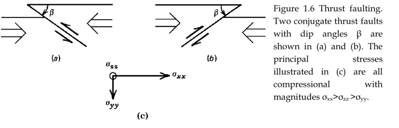
We will first consider thrust faulting (Figure 1.5 c), which occurs for example when the oceanic lithosphere is thrust under the adjacent continental (or oceanic) lithosphere at an ocean trench. Thrust faulting also plays an important role in the compression of the lithosphere during continental collisions. Idealized thrust faults are illustrated in Figure 1.6. Compressional stresses cause displacement along a fault plane dipping at an angle β to the horizontal. As a result of the faulting, horizontal compressional strain occurs. Thrust faults can form in each of the two conjugate geometries shown in Figure 1.6a and b.

The vertical component of stress σyy is the overburden or lithostatic pressure

(σyy= ρgy). The vertical deviatoric stress σyy is zero. To produce the thrust faults

in Figure 1.6, a compressional deviatoric stress applied in the x direction σxx is

required, σxx> 0. The horizontal compressional stress σxx= ρgy + σxx therefore

exceeds the vertical lithostatic stress σxx>σyy.

Figure 1.6 Thrust faulting. Two conjugate thrust faults with dip angles β are shown in (a) and (b). The principal stresses illustrated in (c) are all compressional with magnitudes σxx>σzz >σyy.

For the fault geometry shown in Figure 1.6 it is appropriate to assume that there is no strain in the z direction. In this situation of plane strain we can use to relate the deviatoric stress component σzz to σxx and we can write

σzz= σxx(3) (1.15)

3_{Poisson‘s ratio}

(25)

25

The deviatoric stress in the z direction is also compressional, but its magnitude is a factor of ν less than the deviatoric applied stress. Therefore the horizontal compressional stress,

σzz = gy + σzz = gy + σxx (1.16)

exceeds the vertical stress σyy, but it is smaller than the horizontal stress σxx.

Thrust faults satisfy the condition σxx>σzz>σyy. The vertical stress is the least

compressive stress.

Just as thrust faulting accommodates horizontal compressional strain, normal faulting accommodates horizontal extensional strain. Normal faulting (Figure 1.5 a) occur for example on the flanks of ocean ridges where new lithosphere is being created. Normal faulting also occurs in continental rift valleys where the lithosphere is being stretched. Applied tensional stresses can produce normal faults in each of the two conjugate geometries shown in Figure 1.7.

The displacements on the fault planes dipping at an angle β to the horizontal lead to horizontal extensional strain. Normal faulting is associated with a state of stress in which the vertical component of stress is the lithostatic pressure σyy=

ρgy and the applied deviatoric horizontal stress σxx is tensional (σxx<0).

Figure 1.7 Normal faulting. Two conjugate normal faults with angle of dip βare shown in (a) and (b). The principal stresses illustrated in (c) have magnitudes related by σyy >σzz >σxx.

The horizontal stress, σxx= ρgy + σxx (1.17)

is therefore smaller than the vertical stress, σyy>σxx.

The plane strain assumption is again appropriate to the situation in Figure 1.7, and Equation (1.15) is applicable. Consequently, the deviatoric stress in the z direction σzz is also tensional, but its magnitude is a factor of  smaller than the

deviatoric applied stress. The total stress,

(26)

σzz= ρgy + σxx (1.18)

is smaller than σyy but larger than σxx. Normal faults satisfy the condition σyy

>σzz>σxx, where the vertical stress is the maximum compressive stress. Both

thrust faults and normal faults are also known as dip–slip faults since the displacement along the fault takes place on a dipping plane.

A strike–slip fault (Figure 1.5b) is a fault along which the displacement is strictly horizontal. Thus there is no strain in the y direction. The situation is one of plane strain with the nonzero strain components confined to the horizontal plane. Two conjugate strike–slip faults are shown in Figure 1.8. The fault planes make an angle ψ with respect to the direction of the principal stress σxx. The fault

illustrated in Figure 1.8a is right lateral and the one in Figure 1.8b is left lateral.

Figure 1.8 Strike-slip faulting in plant. Two conjugate strike-slip faults inclined at an angle ψ to the direction of the principal stress σxxare shown in (a) and (b). The principal stresses illustrated in (c) are related by σzz>σyy>σxx.

The state of stress in strike–slip faulting consists of a vertical lithostatic stress σyy=ρgy and horizontal deviatoric principal stresses that are compressional in

one direction and tensional in the other. The case shown in Figure 1.8 has

σxx<0 σzz>0 (1.19)

One can also have

σxx>0 σzz<0. (1.20)

One horizontal stress will thus be larger than σyy while the other will be smaller.

(27)

27

3. Indicators of stress

σzz>σyy>σxx, (1.21)

while Equation (1.20) gives

σxx>σyy>σzz. (1.22)

For strike–slip faulting, the vertical stress is always the intermediate stress. A special case of strike–slip faulting occurs when

|σxx| = |σzz| = τ0. (1.23)

This is the situation of pure shear. The stress τ0 is the shear stress applied across

the fault. In pure shear the angle ψ is 45◦. The displacement on an actual fault is almost always a combination of strike–slip and dip–slip motion. However, one type of motion usually dominates.

3. Indicators of stress

The techniques for determining the state of stress within the Earth were developed in engineering, geology and energy. From a geological point of view, it is important to know the state of stress inside the Earth in order to understand how the plates move, why, where and when earthquakes occur, why and how the structures are formed.

Information about the state of stress in the lithosphere can be obtained through several methods: geological data and recent volcanic alignments, in situ stress measurements, fault plane solutions of earthquakes.

3.1 Gelogic stress indicators

From a geological point of view, there are different types of data that can be used to determine the in situ stress state, as the orientations of igneous dykes or volcanic alignments, which are formed in a plane normal to the least principal stress (Nakamura, 1977) and fault slip data, in particular the inversion of a set of kinematic indicators (or slickenside data) on the faults. The relationship between the faults and the directions of the principal axes of stress, according to the

(28)

Coulomb fracture criterion, suggests that the fault data may be used to determine the orientations of principal stress. The reliability of each estimate of the stress depends on the nature of the faults and the retention of features that indicate their movement.

3.2 In situ measurements

Numerous techniques have been developed to measure stress in deep. Amadei and Stephansson (1997) and Engelder (1993) discuss many of these measurement methods.

The methods of determining stress orientation from observations in wells and boreholes and stress-induced borehole breakouts which access the crust at depths greater than 100m, are expecially useful. These techniques are based on the observation that when a well or borehole is drilled, the stresses that were previously supported by the exhumed material are transferred to the region surrounding the hole. The resulting stress concentration is explained by the elastic theory.

The most common methods to determine the stress orientations from observations in wells and boreholes are stress-induced wellbore breakouts. The breakouts represent an important source of information thanks to the global distribution of oil exploration wells and since the breakouts can provide information on the stress field in regions where there are no available data of earthquakes or faults.

3.3.3 Earthquake Focal Mechanisms

The earthquake fault mechanisms represent an important tool to study the state of stress acting in a tectonic province at great depth. Consequently, the focal mechanisms have been frequently used to estimate the nature of the stress tensor in the seismogenic zones.

(29)

29

3. Indicators of stress

The focal mechanism describes the radiation pattern coming from the hypocenter of an earthquake and is related to the distribution of amplitude, polarity and/or polarization of the initial impulse of the phases P and/or S coming to the seismic stations located around the epicenter of an earthquake. The orientation of the fault plane and auxiliary plane (which bound the compressional and extensional quadrants of the focal plane mechanism) define the orientation of the P (compressional), B (intermediate) and T (extensional) axes. These axes are sometimes incorrectly assumed to be the same as the orientation of 1, 2 and 3.

If friction is negligible on the faults in question (but higher in surrounding rocks), there can be considerable difference (15-20°) between the P, B and T axes and principal stress directions (McKenzie, 1969). An earthquake focal plane mechanism always has the P and T axes at 45° to the fault plane and the B axes in the plane of the fault.

It is necessary to underline that only for an homogeneous body axes P and T represent the principal axes of stress. The pressure and tension axes give the directions of maximum compression and tension in the Earth only if the fault surface corresponds to a plane of maximum shear. Since this is usually not true, the fault plane solution does not uniquely define the stress tensor orientation (although it does restrict the maximum compression direction to a range of possible angles). Thus, there is not an exact match between P and T axes and the orientations of the maximum compressive stress (1) and minimum compressive

stress (3).

The same stress field may be responsible for dislocations on planes differently oriented. Given a set of focal mechanisms of earthquakes generated by the same stress field, the principal directions of stress can be determined through the use of inversion techniques, based on the slip kinematics and on the assumption that fault slip will always occur in the direction of maximum shear stress on a fault plane (among other Gephart and Forsyth, 1984; Micheal, 1984; Angelier, 1990).

(30)

4. Stress inversion from earthquakes

The orientations of fault planes and slip directions indicated by a population of earthquake focal mechanisms can be used to determine best fit regional principal stress directions and a measure of relative stress magnitudes under the assumption of uniform stress in the source region. These analyses allow for the possibility that failure occurs on preexisting zones of weakness of any orientation. The idea is to determine a uniform stress field compatible with the different failure mechanisms that characterize several earthquakes.

However, if there are a variety of different focal mechanisms within a region of uniform stress, then both the principal stress directions and a measure of relative stress magnitudes may be determined. This is possible because on each fault plane, slip occurs in the direction of resolved shear stress (Bott, 1959); with this constraint each observation places a strong restriction on the stresses that generated the fault motion. It happens that each focal mechanism is consistent with only a relatively limited family of stress tensors. By inspecting the overlap of families of stresses associated with a number of focal mechanisms, we can define the range of stresses which may have acted over the region.

The principal stress orientations and a scalar which describes the relative magnitudes of the principal stresses can be determined directly from earthquake focal mechanisms through the use of inversion techniques (Armijo and Cisternas, 1978; Ellsworth and Zhonghuai, 1980; Angelier, 1984; Gephart and Forsyth 1984; Michael 1987a,b).

The basic assumptions of these methods are:

- the stress orientation is spatially uniform within the volume containing the event locations;

- the tangential traction on fault plane is parallel to the slip direction; - enough variety on the fault plane orientations.

The accuracy of these inversion techniques depends on the uncertainty of the focal mechanisms and the fault/auxiliary plane ambiguity.

(31)

31

4. Stress inversion from earthquakes

In Ellsworth and Zhonghuai (1980) method the orientation of the fault plane is taken as perfectly known, and the inverse method involves minimizing, in a least squares sense, the component of shear stress perpendicular to the observed slip direction (or, equivalently, minimizing the sine of the angle between the observed and predicted slip directions) by adjusting the orientation and relative magnitude of the (uniform) principal stresses. This is not the appropriate minimization for earthquake focal mechanism data because it implicitly assumes that the only errors are in the measurement of the direction of slip on the plane, whereas there is often substantial uncertainty in the orientation of the fault plane as well.

Angelier et al., (1982) develop a technique which allowed for error in the orientation of the fault plane. Armijo and Cisternas (1978) developed an alternative approach in which they assumed that the data were exact but that the stress tensor varied in the region of study. They then found the orientation of the principal stresses that minimized the variations required in the relative sizes of the stresses needed to fit the data perfectly. But in this approach there clearly are errors in the observations and non-uniformity in the stress tensor may involve variation in principal stress directions as well as variation in stress magnitudes.

All these inversion techniques, when applied to earthquake focal mechanism data suffer from uncertainty as to which nodal plane is the true fault plane. These methods require that the investigator select the preferred nodal plane from each fault plane solution. Of course, normally this is done on the basis of knowledge of the local geology and tectonics. Often, however, there is no objective means to make this selection.

Gephart and Forsyth (1984) method automatically identifies one the preferred nodal plane from each focal mechanism as a more reasonable fault plane than the other for a given stress model following a grid search methodology.

The algorithm developed by Michael (1987a) is based on that formulation. The basic characteristic of this algorithm is the computation of the confidence limits

(32)

of the principal stress axes directions. Confidence limits are computed by a statistical tool known as bootstrap resampling.

The peculiarity of the technique developed by Rivera et al., 1990 is to obtain the stress tensor, not from previously determined focal mechanisms, but rather from the original data of polarities of P arrival and take-off angles for source- station pairs. This method could be useful when the number of the polarities is scarce to compute reliable focal mechanisms.

4.1 Stress tensor from initial polarities of a population of

earthquakes

An algorithm for the simultaneous estimation of the orientation and shape of the stress tensor and the individual fault plane solutions for a population of earthquakes will be now introduced. It corresponds to a synthesis of the methods used by Brillinger et al., (1980) to obtain focal mechanisms and by Armijo and Cisternas (1978) for stress tensor analysis in microtectonics. The input data are the polarities of the P arrival and take-off angles for the set of source-station pairs. The method distinguishes, in general, which one of the nodal planes corresponds to the fault and gives the direction of the slip (Rivera L. and Cisternas A., 1990).

3.2.1 The Method

We used the method of Rivera L. and Cisternas A., (1990) in which the first-motion data, instead of the mechanic solutions, are directly used for inversion. The data are the raw first-motion polarities for a set of events.

The basic assumptions of the method are the same of other methods that found the principal stress orientations directly from earthquake focal mechanisms(e.g., Gephart and Forsyth 1984; Angelier 1984; Michael 1987;).

(33)

33

4.1 Stress tensor from initial polarities of a population of earthquakes

 [ ] (1.29)

We can obtain this form from geographic coordinates x‘, y‘, z‘ after a rotation using appropriate Eulerian angles (, , ).

The coordinate change after the rotation is represented by the matrix (Goldestein, 1959):

[

         

] (1.30)

To describe the relative magnitudes between three principal axis we define the parameter R = (z- x)/ (y- x) with y>x (Armijo and Cisternas, 1978; Armijo

1982). The R-value is a scalar quantity describing the relative stress magnitudes (the shape of stress ellipsoid).

And under specific conditions (when z-axis is near the vertical, <15°), we can interpret R directly with the tectonic regime (for example with R=0 we have uniaxial compression or with R=1 uniaxial extension (Armijo 1968)).

If for example R > 1 we have z>y>x and so z= 1 ;y= 2 ; x= 3 .

If 0< R < 1 we have y>z>x and so y= 1 ;z= 2 ; x= 3.

(34)

It is convenient to express this quantity through an angle r (-/2, /2) , the

new variable is defined by:

( √ ( )) (1.31) And so under specific conditions, we have compression with r (-/2, -/6),

slip with r (-/6, /6) and extension with r (/6, /2).

Thus, we can describe the state of stress with these three angular parameter , ,

, r .

The method is based on two fundamental hypotesis. The first one is the ―Bott’s hypothesis”:

we assume that the slip vector (t) on the fault plane is parallel to the tangential stress ( St).

The fault plane is described by the unit normal vector n = (l, m, n) T_{where l,m,n}

are the components in the system of the principal axes of stress.

We define the stress acting on this fault S = ._{n and we decompose S in a normal}

and tangential component :

Sn = (ntS) n = (ntn ) n (projection of S on n) (1.32a) St = S – Sn= .n - (ntn ) n (1.32b) and so [ ] [ ( ) ( ) ( ) ] (1.33)

and for the three direction

(St)x = (x(1 - l2) - ym2 - zn2) l = ... = (y - x) (- (m2+n2 R)) l

(St)y = (y - x) (1- (m2+n2R)) m

(St)z = (y - x) (R- (m2+n2 R)) n

We defined K = m2_+n2_{R and so S}_t_{= (}_y_-_x_{) ( -Kl , (l-K) m , (R-K)n)}t

(35)

35

[

( )

( ) ] (1.34) with R = (z- x)/ (y - x) and K = m2 +n2 R

The normal unitary vector in geographic coordinates is

n‘ = (sin  sin s, -sin  cos s, cos )t (1.35)

The relation n = Mn‘ allows us to move on to the coordinates system of principal axis (l,m, n) using the rotation matrix M in (1.34) to found t.

It must be given to geographical coordinates across the relation t‘ = M t .

To resume the Bott‘s hypotesis, we have slip vector as a function of the parameters ,  , , R , s , .

The second hypotesis is ―double couple point source‖.

The theoretical amplitude of the P-wave radiation pattern for a double couple point source is (Aki and Richards, 1980):

AP= 2 (rtn) (rtt) (1.36)

Where r is the unit vector in the source-observer direction. This amplitude is a function of the orientation of the fault plane (n), and of the orientation and shape of the stress tensor (,  , ; R).

Forward problem

Then the forward problem can be defines in the following manner: suppose we know the stress parameters and we assume a fault plane corresponding to the i-th eari-thquake (ni). Then we compute the unit slip vector ti and hence the polarity

Yij of P arrival at the j-th station in this way : Yij = sign (Aij)

Where Yij = + we have compression and where Yij = – dilatation

Yij = Yij ( , , ; s(i),  (i) ; (j), i(j) )

where , ,  describe the orientation of stress tensor; s(i),  (i) describe the fault

plane for each earthquake; and (j), i(j) describe the position of the station on

(36)

Inverse problem

For our problem, given a set of polarities Yij of the initial motion of waves from

N earthquakes recorded at M stations, our aim is to obtain the orientation and the shape of the stress tensor that is compatible with it and the fault plane of each individual earthquake.

Rivera formalized this problem with a probabilistic approach using a maximum likelihood algorithm (Brillinger et al., 1980).

The model parameters are the 3 orientation parameters, , , , for the stress tensor, 1 parameter for the stress ratio R and 2N parameters, si and i with

i=1,2,...N, for the fault planes where si and i are strike and dip of the fault plane

of event i, and N is the number of events used for the inversion.

Then if we want to represent these parameters by a vector we can write m= (,  ,

, R,si, i =1,2,...N).

The algorithm described by Rivera L. and Cisternas A. (1990), the likelihood function L(m) is defined to measure the agreement between the first-motion data and the predicted polarities. In the definition of L, the contribution of each polarity is weighted as a function of the amplitude of the predicted P-wave radiation pattern.

The sample space is the set of all the possible outcomes of measuring polarities at the given source-station pairs. The probability of having a compression at a given station from a given earthquake is

P =  + (1 - 2 )  ( A) (1.37) Where  is a parameter that allows for

errors in reading polarities (  [0, 0.5] ); 

is the normal cumulative function and  is a factor dependent on the amplitude of the signal (distance, magnitude, quality factor) and can be interpreted as an indicator of the accuracy of the take-off angle of the ray.

(37)

37

The probability to obtain a coherent lecture (A positive) is larger than 0.5. It increases with the size of the radiation pattern and tends to (1-ε). Instead for the negative lecture the probability is smaller than 0.5 (it tends to ε) [0, 0.5]. For a seismogram with a good signal/noise ratio  is equal to 0.

The parameter  governs the slope of this probability. With a large  the function is like a step.

The probability of reading a dilatation is 1-P (Y = +) . The logarithm of the probability that a set of observed polarities Yij correspond to a model producing

a theoretical amplitudes Aij is given by the expression (Buforn, 1985):

L = - log ½  (1+Yij (1-2) 2(Aij) -1  (1.38)

Where L is a function of the parameters of the model through the theoretical amplitudes Aij.

The parameters of the stress tensor and the orientation of the fault planes are chosen so that they maximize the likelihood function L. An initial model (, , ,

R, ni) is modified in an iterative process up to the point where a given

convergence criterion is satisfied. Since the dimension of the parameter space involved in the inversion is large, the calculations were carried out by using a quasi-Newton method (Harwell Scientific software Library).

The algorithm takes a given starting model m0, uses the gradient of L to sweep the model space, improves the fit, and iterates until a small enough gradient is found (Rivera and Kanamori 2002). Because of the binary nature of the data and the non-linearity of the problem, the procedure just described does not necessarily converge to the best solution, and can settle at a local minimum.

Error estimation

Rivera et al., 1990 followed the maximum likelihood procedure described by Brillinger et al., (1980) in the estimation of uncertainties of the model parameters. We compute the information matrix I()

 : estimated value of the parameters of the model (R, Euler‘s angles, and position of each poles of the fault planes on the sphere).

(38)

() *∑ (



 )

{ ( )}+ (1.41)

Where the average is performed over all the possible configurations in the sample space, and the sum is made over all the pairs station-source.

The covariance matrix is then obtained as the inverse of the information matrix C = I() -1 _{and then we can estimate the confidence ellipses of the poles of the fault}

planes on the focal sphere, and of the main axes of the stress tensor, together with the variance of the shape factor.

Analysis of the discrimination between fault and auxiliary planes

We have seen in the equation (1.34) that the stress tensor determines the slip vector on a given fault plane, and hence the second nodal plane of the focal mechanism. The action of the same stress tensor on this second plane will not general, a slip vector orthogonal to the first plane.

The discrimination is not possible in some cases:

o If the stress tensor has a cylindrical symmetry (R= ; R=0 ; R=1)

o if the normal to the fault plane happens to be orthogonal to one of the main axis of the tensor (in other words, if the fault plane passes through one of the principal axes of stress (l=0, m=0, n=0))

(39)

Chapter 2 Geological and geophysical setting

of the investigated area

1. Introduction

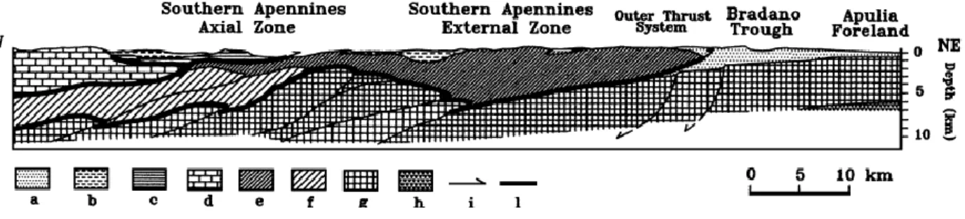
The Campania-Lucania region is located in the axial portion Southern Apennines, an Adriatic-verging fold-and-thrust belt, tectonically stacked over the flexured southwestern margin of the Apulia foreland.

The chain is located between the Tyrrhenian back-arc basin to the west and the Bradano foredeep to the east. During the Middle Miocene - Late Pliocene, several compressive tectonic phases, associated with the collision between the African and European margins, caused thrusting and stacking of different units toward stable domains of the Apulia foreland (whose sedimentary cover is formed by the Apulia Carbonate Platform, ACP). From Late Tortonian to Early Pleistocene, the system rapidly migrated to east as a consequence to ―eastward‖ retreat of the sinking foreland lithosphere (Malinverno and Ryan, 1986; Patacca and Scandone, 1989, Patacca et al., 1990).

The current structural complexity of the chain is also due to the different paleogeographic domains involved in the Southern Apennines tectonic units. The basinal facies successions allowed ductile deformation, while the carbonate platform successions mainly show a brittle behavior (D‘Argenio et al., 1974; Improta et al., 2003). In addition, the deformation did not proceed cylindrically, but it was characterized by out-of-sequence thrust-propagation processes (Roure

et al., 1991). During the Late Pliocene - Early Pleistocene time span, the

fold-and-thrust belt evolved tectonically by forming different arcs: the NNW-SSE-trending Molise-Sannio arc, to the north, and the WNW-ESE-NNW-SSE-trending Campania-Lucania arc, to the south.

(40)

Since the Middle Pleistocene, the fold-and thrust-belt started to uplift and to be affected by a NE-SW extensional tectonic regime, which caused the development of extensional fault systems along the core of the chain, which cut the preexisting compressional stack further complicating the internal geometry of the thrust belt. The extensional stress regime is still active along the chain axis, as indicated by the analysis of surface geological indicators, as well as of breakout, seismic and GPS data (Pantosti and Valensise, 1990; Frepoli and Amato, 2000; Montone et al., 2004; DISS Working Group, 2010; Devoti et al., 2008; Pasquale et al., 2009; De Matteis et al., 2012 under revision) and is responsible for the present-day seismicity in the Apennines chain. The background seismicity is mainly distributed along the axis of the chain and it is characterized by low to moderate magnitude earthquakes. It has to be noted, however, that the seismicity that occur between the Apennines chain and the Adriatic foreland may nucleate at depth between 10 and 25 km (Valensise et al., 2004).

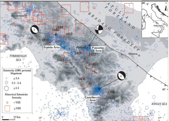
In particular, the Campania-Lucanian region is one of the most active seismic zones of the Apennines chain. Large destructive earthquakes occurred both in historical and recent times in this region, which was struck on 23 November 1980 by one of the strongest events (M6.9) in the past century. Detailed seismological studies on this earthquake have demonstrated the complexity of its source mechanism, which consists of at least three normal-faulting ruptures nucleated in a time range of 40 s on approximately 60 km long, NW-SE striking, three individual fault segments (Westaway and Jackson, 1987; Bernard and Zollo, 1989; Pantosti and Valensise, 1990; Amato and Selvaggi, 1993 ).

More than 30 years after this event, the seismotectonic environment that encompasses the fault system on which the 1980 earthquake occurred, shows a continuous background seismic activity including moderate-sized events. Since 1980, a normal faulting mechanism earthquake (ML=4.9) happened within the

epicentral area of the 1980 earthquake on 3 April 1996. Moreover, two moderate magnitude seismic sequences occurred between 1990 and 1991 (ML=5.2 and

(41)

47

1. Introduction

the SE of the 1980 Irpinia aftershock area (Ekstrom, 1994). These latter sequences were characterized by dextral strike-slip faulting mechanisms and E-W strike (Di Luccio et al., 2005, Boncio et al., 2007).

The crustal tectonic setting of the Campania-Lucanian region has been defined by several geological and geophysical studies like tomographic studies (Amato and Selvaggi 1993, Chiarabba and Amato 1994, De Matteis et al., 2010), analysis and joint interpretation of gravity data, seismic reflection lines and subsurface information from many deep wells (Improta et al., 2003), in many cases carried out for hydrocarbon exploration purposes (Mostardini and Merlini, 1986; Patacca and Scandone, 1989, 2001; Casero et al., 1991; Roure et al., 1991; Menardi Noguera and Rea, 2000; Scrocca et al., 2005).

The inferred crustal models show considerable lateral variations of the medium properties moving perpendicularly to Apennines belt. This variability is consistent with the presence of the Apulia Carbonate Platform, Western Carbonate Platform and basinal deposits successions, which form different tectonic units piled in the thrust stack. In addition, major lithological variations are evident along the strike of the mountain range, the most relevant being an abrupt deepening of the Apulia Carbonate Platform to the southeastern part of the investigated region (Improta et al., 2003).

In the epicentral region of the 1980 event, the structural setting of the buried Apulia Carbonate Platform and underlying Permo-Triassic basement appears to be correlated with the P-wave velocity variations in the upper crust and with the aftershocks distribution. The structural highs of the Apulia Platform correspond to high-velocity regions, where aftershocks and coseismic slip of the mainshock are concentrated. This correlation suggests that the lithological heterogeneities in the upper crust, and in particular the Apulia Carbonate Platform units play a primary role in the rupture propagation and aftershocks distribution (Amato and Selvaggi, 1993; Improta et al., 2003).

(42)

2. The Southern Apennines

Moving from north-east to south-west, i.e. from the foreland to the chain, the Southern Apennines are characterized by four main structural domains: the Apulian foreland, the Bradanica foredeep, the Apennines chain and the Tyrrhenian basin (Patacca and Scandone, 1987; Figure 2.1).

Figure 2.1 Simplified geologic map of Southern Apennines (from Scrocca et al., 2005). Letters refer to deep wells (A, Puglia 1; B, Gaudiano 1; C, Bellaveduta 1;D, Lavello 5; E, Lavello 1; F, S. Fele 1; G, M. Foi 1; H, Vallauria 1; I, S. Gregorio Magno 1; J, Contursi 1; K, Gargano 1).

The Apulian foreland, with its Meso-Cenozoic sedimentary cover (ACP - Apulia Carbonate Platform), is considered a stable area with respect to the Apennines, being only marginally involved in the tectonic movements that affect the Apennines chain. The few not negligible active faults that characterize this foreland are mainly E-W trending, subvertical right-lateral shear zones (e.g., the Mattinata fault in the Gargano promontory). The stratigraphic succession consists of continental and shallow marine Permo-Triassic deposits (Verrucano).