Parental Divorce and Students' Performance:
Evidence form Longitudinal Data
Anna Sanz de Galdeano, Daniela Vuri
CEIS Tor Vergata - Research Paper Series, Vol.
27, No. 81, March 2006
This paper can be downloaded without charge from the Social Science Research Network Electronic Paper Collection:
http://ssrn.com/abstract=897504
CEIS Tor Vergata
RESEARCH PAPER SERIES
Parental Divorce and Students’ Performance:
Evidence from Longitudinal Data
∗†Anna Sanz de Galdeano
csef, university of salerno
Daniela Vuri
university of florence, child and iza
4863 words
Abstract
In this paper we analyse data from the National Education Longitudinal Study to investigate whether experiencing parental divorce during adolescence has an adverse impact on students’ performance on standardized tests. To ac-count for the potential endogeneity of parental divorce we employ double and triple differences models that rely on observing teenagers from intact and di-vorced backgrounds before and after the divorce occurs. We find that parental divorce does not negatively affect teenagers’ cognitive skills. Our results also suggest that cross-section estimates overstate the detrimental effect of parental divorce.
Keywords: Divorce; Difference in differences; Cognitive Development. JEL Classification: J12; C23.
∗We thank the U.S. Department of Education’s National Center for Education Statistics for access
to the public use NELS data and Jennifer Thompson for kindly answering our questions about the data files. Seminar participants at the EUI, UNICEF and CSEF gave very helpful comments on earlier drafts.
†Address correspondence to: Anna Sanz de Galdeano, CSEF, University of Salerno, Via Ponte
don Melillo, 84084, Fisciano (SA), Italy, E-mail: [email protected], Tel.: 39-089-962831, Fax: 00-39-089-963169. Daniela Vuri, Economics Department, University of Florence, Via delle Pandette 9, Edificio D6, Florence, Italy, E-mail: [email protected], Tel.: 4374567, Fax: 00-39-055-4374905. Anna Sanz de Galdeano acknowledges financial support from a European Community Marie Curie Fellowship (http://www.cordis.lu/improving). The authors are responsible for information communicated and the European Commission is not responsible for any view or results expressed.
1
Introduction
Establishing whether parental divorce has a causal negative effect on children’s out-comes is a crucial issue for the evaluation of divorce and family laws. Several states in the U.S. have recently started tightening divorce requirements, reversing the liber-alizing trend in divorce laws that began around 1970. 1 The proponents of tightening the divorce regime often argue that making divorce easier has negative consequences for children. However, as pointed out by Gruber (2004), this argument relies on three implicit suppositions. First, that easier divorce regulations cause an increase of di-vorce rates. Empirical work on this supposition has reached mixed conclusions: while Friedberger (1998) finds that there is an impact of unilateral divorce on divorce rates in the U.S., the evidence presented by Wolfers (2003) indicates that the increase in divorce rates is only transitional, disappearing after a decade. Second, that changes in divorce regulation only have an impact on families and children through their effect on the propensity to divorce. The third supposition that drives criticism of easier divorce regulations, on which this paper focuses, is that divorce has an adverse impact on children.
There is an enormous literature that finds that experiencing parental divorce is negatively related to a wide variety of children’s outcomes such as educational at-tainment, fertility choices (specially non-marital birth during teenage years), future earnings, employment status and welfare recipiency among others (many of these
stud-1Unilateral divorce, which requires the willingness of only one spouse to divorce, rather than
the consent of both spouses, was rare before the late 1960s but was in place in most states by the mid-1970s.
ies are reviewed in Amato and Keith 1991, and Haveman and Wolfe 1995). However, this large literature can hardly be interpreted causally because divorce is associated with socioeconomic characteristics that also determine children’s attainments. For instance, there is a negative relationship between divorce and men’s earning ability (Sander 1986). Moreover, even if socioeconomic information is available, the ques-tion of causality is further complicated because it is unlikely that these observable variables can fully capture the unobservable differences that may exist between fam-ilies that choose to divorce and intact famfam-ilies; for example, it may be the conflict associated with divorce, rather than divorce per se, what leads to children’s inferior outcomes. Therefore, it is easy to overstate the detrimental impact of divorce.
Several studies have stressed the difficulties associated with the endogeneity of parental divorce. Manski et al. (1992) present and interpret alternative estimates of the effect of family structure on high school graduation, obtained under differing assumptions about the process generating family structure and high school outcomes. Sandefur and Wells (1997) and Bjorklund et al. (2004) use sibling data to control for unmeasured characteristics of families that are common to siblings. Corak (2001) assumes that parental loss by death is exogenous and argues that children with a bereaved background offer a benchmark to assess the endogeneity of parental loss through divorce, considering that any difference between the outcomes of individuals from bereaved and divorced backgrounds represents the consequences of an endogene-ity bias. In a related paper, Lang and Zagorsky (2001) also consider parental death as an exogenous source of parental absence. Gruber (2004) states that “what is re-quired to appropriately identify the impact of divorce is an exogenous instrument that
causes some families to divorce and others not, based on a factor independent of the determinants of their children’s outcomes” (p. 806). However, a valid instrument is hard to find in this context and not even changes in divorce laws could be considered as such if, as suggested by Stevenson and Wolfers (2003), changes in divorce regimes may directly affect the nature of intrafamily bargaining, with potential implications for children’s outcomes.
In this paper we revisit the question of whether parental divorce leads to children’s worse outcomes using a nationally representative sample of youths from the National Education Longitudinal Study of 1998 (NELS: 1988). We expand the existing em-pirical literature in two important ways. First, we examine the relationship between parental divorce and student’s performance on standardized tests. Test scores are often used to evaluate the performance of students, teachers and schools (Kane and Staiger 2002) and many studies have shown that scores on cognitive tests taken during adolescent years are important determinants of future wages and employment proba-bilities (Murname et al. 1995; Neal and Johnson 1996; Cawley et al. 1997; Currie and Thomas 2001; Zax and Rees 2002). There is also evidence that the greater dispersion of cognitive test scores in the United States plays a role in explaining the fact that wage inequality is higher in the U.S. than in Europe (Blau and Kahn 2004). Moreover, psychologists (e.g. Harris, 1983) have shown that children’s scores in cognitive and de-velopmental tests are strong predictors of later outcomes. This voluminous literature suggests that test scores are important variables to examine.
Second, our empirical approach, which is different from methods used in the lit-erature, allows for the possibility that parental divorce is correlated with unobserved
family characteristics that may influence children’s outcomes. The longitudinal nature of the NELS allows us to account for the potential endogeneity of parental divorce by using double and triple differences models that rely on observing the outcomes of chil-dren from intact and divorced backgrounds before and after the divorce takes place.
Our main finding is that parental divorce does not adversely affect teenagers’ cog-nitive skills. Teenagers from divorced families appear to perform worse than their counterparts from intact families before the divorce actually takes place. Our results also suggest that cross-section estimates actually overstate the detrimental effect of parental divorce.
The paper proceeds as follows. Section 2 lays out our empirical strategy for iden-tifying the impact of parental divorce on adolescents’ cognitive ability. The data set used is described in Section 3. Section 4 discusses the results and Section 5 offers some concluding comments.
2
Empirical Model
Let Y (i, t) be the outcome of interest for teenager i at time t. As a starting point, let us assume that we observe the population of youths in two periods, t = 1 and t = 2. Between these two periods, some fraction of the population experiences parental divorce. We denote D(i, t) = 1 if teenager i has experienced parental divorce between period 1 and period 2 and D(i, t) = 0 if teenager i’s parents are still married in period 2. Since teenagers are only exposed to parental divorce after period 1, D(i, 1) = 0 for all i by definition and youth with D(i, 2) = 1 are called treated while those
with D(i, 2) = 0 are called controls. The following formulation of the difference-in-differences (DID) framework is based on that in Ashenfelter and Card (1985) and Abadie (2005). Suppose that Y (i, t) follows a components-of-variance scheme:
Y (i, t) = δ(t) + α·D(i, t) + η(i) + υ(i, t) (1)
where δ(t) is a time-specific component, α is the impact of parental divorce and υ(i, t) is a serially uncorrelated transitory component. Finally, η(i) is an individual-specific component that represents unobserved pre-disruption characteristics such as the con-flict between the parents or the stress and friction associated with an unhappy family life. If D(i, t) is independent of η(i) and υ(i, t), then the difference in test scores between treated and controls in t = 2 will estimate the effect of parental divorce α. However, D(i, t) is very likely to be correlated with η(i).
Given the longitudinal nature of the NELS:1988, which we describe in detail in the next section, both pre-divorce and post-divorce data are actually available. Hence, one could control for η(i) by comparing the scores of teenagers from divorced families with the scores of these same teenagers before the divorce occurs. However, this comparison might be contaminated by temporal variation in test scores that is not due to parental divorce. Since not all the teenagers in the population experience parental divorce, teenagers from intact families can be used to identify temporal variation in the outcome that is not due to divorce. This is the main idea behind the DID estimator.
Differencing (1) with respect to t we obtain:
Y (i, 2)− Y (i, 1) = δ + α·D(i, 2) + (υ(i, 2) − υ(i, 1)) (2)
P (D(i, 2) = 1|υ(i, t)) = P (D(i, 2) = 1) for t = 1, 2. Under this restriction, the least square estimator of α is the sample counterpart of the following equation:
α = {E[Y (i, 2)|D(i, 2) = 1] − E[Y (i, 2)|D(i, 2) = 0]} − {E[Y (i, 1)|D(i, 2) = 1] − E[Y (i, 1)|D(i, 2) = 0]}
Note that P (D(i, 2) = 1|υ(i, t)) = P (D(i, 2) = 1) for t = 1, 2 implies that (υ(i, 2) − υ(i, 1)) is mean independent of D(i, 2) and therefore that, in absence of parental di-vorce, the average test scores for the treated would have experienced the same varia-tion as the average test scores for the controls. This assumpvaria-tion may be implausible if treated and controls are unbalanced in covariates that are thought to be associated with the dynamics of the outcome variable. Hence, we introduce covariates linearly in equation (2):2
Y (i, 2)− Y (i, 1) = δ + α·D(i, 2) + X0(i)π + (υ(i, 2)− υ(i, 1)) (3)
where π = π(2) − π(1) and X(i) is a vector of observed characteristics that are as-sumed uncorrelated with υ(i, t). Note that the model is now identified under the conditional restriction P (D(i, 2) = 1|X(i), υ(i, t)) = P (D(i, 2) = 1|X(i)) for t = 1, 2. In other words, if non-parallel test score dynamics for the treated and the controls can be explained by including covariates, then model 3 is identified. Accordingly, the plausibility of this condition relies on the inclusion of a rich set of covariates. How-ever, if the dynamics of test scores depend on unobservables, or, in other words, if the unobserved variation associated with divorce is not fixed over time, identification
2Heckman et. al. (1997) and Abadie (2005) propose DID estimators based on conditional
breaks down.3 One way to assess the plausibility of the identifying condition is to use data on more than one pre-divorce period (that is, use data for t = 0 as well) to apply the DID estimator to at least two pre-divorce periods and test that α is equal to zero:
Y (i, 1)− Y (i, 0) = γ + α·D(i, 2) + X0(i)τ + (υ(i, 1)− υ(i, 0)) (4)
where γ = γ(1)−γ(0) and τ = τ(1)−τ(0). Alternatively to the DID model and in order to relax its identifying condition, we also apply a difference-in-difference-in-differences (DIDID) estimator to the three data periods. The DIDID model, which is obtained by substracting equation 4 from equation 3, is identified under the more general condition that unobserved factors jointly influencing cognitive development and the probability of divorce grow at a constant rate.4
3
Data
The individual data used in this paper are from the National Educational Longitudi-nal Study of 1988 (NELS:88), a continuing study sponsored by the U.S. Department of Education’s National Center for Education Statistics. A nationally representative sample of 24,599 8-th graders were first surveyed in 1988. Many of these same stu-dents were re-surveyed through four follow-ups in 1990, 1992, 1994 and 2000.5 The first follow-up includes responses from approximately 17,500 of the students from the
3Or, more generally if it does not grow at the same rate on average for the treated and the control
groups.
4Note that this growth rate can differ between the treated and the control groups.
5The last two follow-ups are not used in this analysis because the outcome of interest is collected
first wave while the second follow-up includes approximately 16,500 students from the original cohort.
On the questionnaires, students reported on a range of topics including school, work and home experiences. Depending on the year, data were also collected from parents, schools and teachers. In addition, for the three in-school waves of data collection (1988, 1990 and 1992), cognitive tests were administered. The administration of cognitive tests in multiple waves allows us to analyse the impact of changes in teenagers’ lives on their performance on standardized tests.
The NELS:88 cognitive test battery consists of multiple choice tests in four subject areas: reading comprehension, mathematics, science and history/citizenship/geography. In the base year, all students received the same set of tests. In order to avoid “ceiling” and “floor” effects, that is, many students getting either all items correct or incorrect, the reading and mathematics tests in the first and second follow-ups were tailored to students’ ability levels in the previous wave. Item Response Theory was used to develop scores that are on the same scale and thus can be compared to measure gains in achievement over time. The maximum possible scores that a teenager could achieve are 81 in mathematics, 38 in science, 47 in history and 54 in reading.
Our identification strategy, described in the previous section, requires observing teenagers’ outcomes before and after parental divorce.6 Therefore, we depart from a sample of approximately 16,500 teenagers who participated in the first three waves of the data. Furthermore, our estimation strategy requires having information on test
6Note that our double and triple differences models do not allow us to examine adult labour market
scores in at least two points in time and being able to code family transitions during high school. A unique feature of the NELS:88 data is that youth who leave high school prior to graduation continue to be interviewed throughout the longitudinal study. It is therefore possible to include in our analyses dropouts who are not represented in other national school-based surveys. Moreover, students who had transferred out of the school from which they had initially been selected were subsampled and reinterviewed. It is also worth noting that all statistics presented in this paper are weighted using NELS:88 weights, which attempt to compensate for unequal probabilities of selection and to adjust for the effects of nonresponse.7
In order to code family transitions, we have used information from the parent questionnaires and we have contrasted it with the information provided by students. We have classified families into two broad categories in 1988: intact families (with both biological parents) and non-intact families (stepfamilies and single parent families). For the majority of our analyses, which require observing teenagers before and after parental divorce, we have departed from the sample of students from intact families in 1988 and then identified those who experience parental divorce during high school and those whose families remain intact.8 In order to focus on the impact of parental divorce,
7Weights are calculated in two main steps. In the first step, unadjusted weights are calculated
as the inverse of the probabilities of selection, taking into account all stages of the sample selection process. In the second step, these initial weights are adjusted to compensate for nonresponse; such nonresponse adjustments are typically carried out separately within multiple weighting cells. The nonresponse adjustment factor was intended to adjust for the fact that some of the sampled students did not participate, that is, did not return a completed questionnaire.
we exclude teenagers who experience parental death during high school. Regarding multiple transitions, we have counted families that undergo divorce and subsequently remarry while their child is in high school as divorced families, but our results are unchanged when eliminating these families.
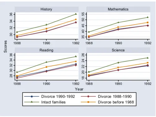
Figure 1 displays mean test scores for teenagers from persistently intact families and for teenagers whose parents divorce before 1988, between 1988 and 1990 and between 1990 and 1992. A number of features are worth noting. First, cognitive test scores rise with age and schooling. This is consistent with the findings of Cawley et al. (1997). Second, teenagers with a divorced background perform worse than their counterparts from intact families. Finally, at least part of this gap is visible before the divorce actually takes place. Accordingly, it is possible that the endogeneity of parental divorce is generating this difference. For example, conflict between parents may lead to both divorce and teenagers’ worse outcomes. Another possibility is that parents who are less committed to their families may be more likely to divorce and may also invest less time in their children.
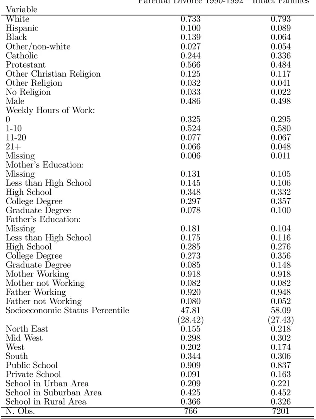
Alternatively, it is possible that the difference in test scores is due to background differences between teenagers from divorced and intact families. The NELS:88 ques-tionnaires also provide additional information on family and school characteristics. Table 1 presents the means and standard deviations of the main variables employed in the statistical analyses for the sample of teenagers from intact two-parent families and for those who experienced parental divorce between 1990 and 1992.9 Note that
separation and divorce. Hence, in what follows we make no distinction between teenagers from divorced and separated family backgrounds.
30 32 34 36 35 40 45 50 55 28 30 32 34 36 18 20 22 24 26 1988 1990 1992 1988 1990 1992 1988 1990 1992 1988 1990 1992 History Mathematics Reading Science Divorce 1990-1992 Divorce 1988-1990 Intact families Divorce before 1988
Sc
or
es
Year
Figure 1: Mean Test Scores by Year
sample sizes correspond to the analysis of mathematics test scores but they do slightly differ for the other examinations. Some observations are lost due to missing informa-tion on background and/or school characteristics. In our analyses, we have included dummy variables indicating observations for which information was missing on some characteristics such as parental education, age and place of birth. 10
In line with the idea that children of divorce come from more disadvantaged back-grounds than children from intact families, Table 1 indicates that teenagers from intact families have better educated parents. Moreover, teenagers of divorce come from fam-ilies at the 48th centile of the socioeconomic distribution (based on the entire NELS sample), while the average in the intact families sample is at the 58th centile.11 Table
teenagers who experienced parental divorce before 1988 and between 1988 and 1990.
10However, our results are robust to the exclusion of these observations.
house-1 also reveals that teenagers from divorced families are more likely to work more than 11 hours per week, be Black or Hispanic, not being catholic, live in the South or in the West and attend public schools and schools located in rural areas.12
Finally, it is worth remarking that the fact that we analyse teenagers during the high school period may lead to estimate an effect of parental divorce which could be either larger or smaller than the effect of divorce for younger children. On the one hand, parental divorce might have a more detrimental impact for younger children. On the other hand, Painter and Levine (2000) suggest that if the survey is taken during a transitory period after parental divorce, we may overestimate the test scores gap due to this traumatic shock.
4
Does Parental Divorce Reduce Teenagers’
Cog-nitive Skills?
4.1
Estimation and Basic Results
As a benchmark for later comparisons, equation (1) is first estimated using 1992 in-formation on test scores. OLS coefficient estimates, reported in Table 2 (column 1, row 1 of each panel), are negative and statistically significant at the 1% level for all four examinations. It is found, for example, that teenagers who experience parental divorce between 1990 and 1992 perform 6 points worse than their counterparts from
hold income.
12We have also checked that the characteristics of our analytical sample do not substantially differ
intact families on the 1992 mathematics test. To assess the magnitude of these effects, we also use the student’s 12th-grade percentile rank based on her 12th-grade score in all the tests as dependent variables. The results of these analyses, shown in column 2, suggest that experiencing parental divorce reduces test score ranks in mathematics, science, history and reading by 12, 11, 11 and 7 percentile points, respectively.
Part of the estimated difference in test scores between teenagers from divorced and intact families may be due to the observed background differences highlighted in Section 3. Hence, we now explore whether these findings are robust to the inclusion of controls.
First, consider the coefficients on some of the explanatory variables, reported in Table 3. There are statistically significant and negative impacts on the mathematics score from being Black or Hispanic, working more than 21 hours per week and attend-ing a public school. On the other hand, havattend-ing highly educated parents, comattend-ing from families with high socioeconomic status, having a working mother, being male and not living in the South appear to increase the mathematics score.13
Regarding the impact of parental divorce, conditional estimates for all four exami-nations are also reported in Table 2 (columns 3 and 4, row 1 of each panel). It is found that parental divorce is associated with a decrease of approximately 4-5 points in the mathematics, science and history percentile ranks, while the reading rank is only re-duced by approximately 2 percentile points and it is not statistically significantly. The results suggest that conditional coefficient estimates are substantially smaller in
ab-13We obtain qualitatively very similar results for the other three examinations, with the notable
solute value than the unconditional estimates displayed in columns 1 and 2. However, they are still negative and (with the exception of the reading examination) statistically significant at standard levels and the associated percentage effects range between 5% (mathematics score) and 2% (reading score). 14
The estimated negative effects so far obtained are generally in line with previous studies on the implications of parental divorce. However, they may overstate the detri-mental impact of divorce if they measure both the effect of parental divorce and the effect of unobserved family characteristics, η(i), associated with divorce. In fact, when equation (1) is estimated using 1990 (10th-grade grade) test scores information (Table 2, row 2 of each panel), it is found that, prior to parental divorce, teenagers whose parents will divorce between 1990 and 1992 perform worse than their counterparts from intact families. This is consistent with the results of Piketty (2003), which reveal that pre-separation children do as bad at school as single-parent children in France.
As a next step in our analysis we use a DID estimator, which is obtained by comparing the change in test scores for teenagers who are exposed to parental divorce with the change in test scores for teenagers from intact families. DID estimates without and with covariates (equations (2) and (3), respectively) are displayed in row 3 of each
14There are alternative ways of assessing the magnitude of the effects. We have also computed the
percentage variation of test scores due to parental divorce as
SN
i=1[( ˆY1i− ˆY0i)/ ˆY0i]
N ∗ 100, where N is the
total number of observations and ˆY1i and ˆY0i denote the predicted value of test scores for individual
i when experiencing parental divorce and when coming from an intact family, respectively. Another way to compute percentage effects that we have considered is to use the ratio between the estimated OLS coeffcients and the corresponding maximum score values for each examination. These results, not reported, lead to essentially the same conclusions.
panel of Table 2. The evidence suggests that parental divorce is associated with a very modest decrease in the mathematics and history ranks of approximately 2 percentile points, respectively. Moreover, even if these estimates are statistically significant, they translate into negligible percentage effects (not reported).
For the science and reading examinations, parameter estimates are very small in magnitude and statistically insignificant at conventional levels of testing. We have also used the sum of test scores as the outcome of interest, finding that the para-meter estimate for the parental divorce variable is very close to zero and statistically insignificant at standard levels. Additionally, we have replicated the previous analyses using teenagers whose parents were divorced by 1988 as the comparison groups. The results associated with this alternative comparison group are remarkably similar and therefore not reported. In sum, the evidence based on the DID estimates suggests that parental divorce does not adversely affect teenagers’ cognitive development. Thus the earlier cross-section results actually overestimate the detrimental impact of parental divorce.
As discussed in Section 2, the DID model used so far assumes that in the absence of parental divorce, test scores of teenagers from intact and divorced backgrounds would have followed parallel paths over time. We have applied the DID estimator to periods 1988 and 1990 in order to assess whether this assumption is plausible. While the results are not reported the evidence is suggestive that this assumption may not always apply, since the estimates of α are negative and in some cases statistically significant at standard levels of testing. Therefore, we now use a DIDID model that identifies our parameter of interest under the more general condition that unobserved
factors jointly influencing test scores and the divorce decision grow at a constant rate. DIDID estimates with and without covariates are reported in Table 4. Parental divorce appears to have a less detrimental impact on math and history scores than implied by the corresponding DID estimates presented in Table 2. For the science and reading examinations, DIDID coefficient estimates are positive and bigger than the corresponding DID estimates displayed in Table 2. However, all estimates are negligible and most of them are statistically insignificant at the 10% level, supporting the previous conclusion that parental divorce does not negatively affect teenagers’ cognitive development.15. This finding is in line with Corak (2001), who uses Canadian administrative data and concludes that, with respect to labor market outcomes such as earnings and use of social programs, the causal impact of divorce is relatively “mild or insignificant”(p. 712). Along the same lines, Lang and Zagorsky (2001) use data from the NLSY and find little evidence that a parent’s presence during childhood affects educational and labor market outcomes.
15The NELS:88 dataset does not contain information on parental marital status after 12th grade.
Therefore, one may be concerned that we are underestimating the impact of parental divorce by including in our control group teenagers from families that will go through a divorce after the high school period. In order to address this issue, we have performed a simple simulation exercise: we have assumed that teenagers from intact families with low test scores are those more likely to experience parental divorce later in life and we have re-estimated our DIDID models by dropping from our sample those teenagers from intact families with test scores in the lower tail of the distribution. The results of this analyisis suggest that in order to find a statistically significant effect of parental divorce one would need to eliminate at least 30% of the teenagers currently classified as belonging to intact families and even in this case the magnitude of the estimated effect would not be bigger than 2.3 percentile points.
4.2
The Impact of Parental Divorce by Adolescent
Charac-teristics
Although our analyses mainly focus on the average effect of parental divorce, it may be that it has little impact on most teenagers but a very important impact on certain groups. Hence, we also evaluate the impact of parental divorce for teenagers with specified characteristics in Table 5.
The results in Table 5 reveal that the effect of parental divorce is very small for all the categorizations of the data examined. We find that coefficient estimates are never statistically significant at standard levels and we cannot reject the hypothesis that the effects are equal for the mutually exclusive groups considered. For the sake of brevity, Table 5 only displays results for the mathematics score. However, an examination of the corresponding findings for the science, history and reading scores indicated that they were remarkably similar. This suggests that the impact of parental divorce does not significantly differ across groups of adolescents.
4.3
Age at Time of Parental Divorce
We have so far analysed the effect of experiencing parental divorce for the population of teenagers whose parents divorced while they were between the 10-th and 12th-grade. However, the impact of parental divorce may be greater if the divorce occurs when children are younger. Moreover, to the extent that regulations that tighten the divorce regime do not avoid divorce but delay it by a few years, it is also interesting to explore the differences between children whose parents divorced while they were between the
10th-grade and 12th-grade grade with children whose parents divorced at earlier ages. Given that cognitive tests were also administered in the 1988 wave of the NELS:88, some evidence on this issue can be provided by estimating the effect of experiencing parental divorce between 1988 and 1990 on the 1990 (10th-grade grade) test scores. The results of this analysis are reported in Table 6.16
All DID coefficient estimates are now negative, including those corresponding to the reading and science examinations, which are positive in Table 2. However, the estimated effects remain very small and statistically insignificant at standard levels in most cases. Moreover we cannot reject the hypothesis that these effects equal those reported in Table 2. This indicates that parental divorce is not more detrimental if it occurs when children are younger, at least as long as they are between the 8-th and 12th-grade grade. This finding is consistent with Cherlin et al. (1995) and Piketty (2003). Cherlin et al. (1995) use British data and find that the timing of parental divorce (ages 7 to 11 versus ages 11 to 16) in a child’s life does not make a difference for young adult outcomes. Piketty (2003) obtains analogous results by analysing French data on school performance.
4.4
“Less Immediate” Effects of Parental Divorce on
Cogni-tive Ability
Thus far, we have estimated the impact of parental divorce on cognitive development in a relatively short interval after the divorce occurs. However, the effect of parental
16Note that in this case it is not possible to use a DIDID model because the NELS:88 did not
divorce may be attenuated over time. Insight into the "less immediate" impact of parental divorce can be found by examining the impact of divorce between 1988 and 1990 on cognitive test scores in 1992, ensuring at least a two-year lag between the dates of the divorce and the examination.17 Table 7 reports the results of this analysis.
For the math, history and reading examinations, it is found that the estimated effects of parental divorce appear to be more detrimental than the more immediate effects displayed in Table 6. However, both effects are very modest and we cannot reject the hypothesis that they are equal. This suggests that the long run and the short run effects of parental divorce do not significantly differ.
5
Summary and Conclusions
This paper examines whether parental divorce negatively affects students’ performance as measured on standardized tests. The negative association between parental divorce and children’s outcomes has been documented extensively. However, this negative relationship may be reflecting unobserved family differences between teenagers from divorced and intact families. In order to account for the endogeneity of parental divorce we employ double and triple differences models which control for the family specific effects operating through the parental divorce decision.
Our empirical work identifies several important results. First, parental divorce does not have a negative causal effect on teenagers’ cognitive development. Our evidence
17It is not possible to analyse a longer time interval because the NELS:88 did not administer
also suggests that the impact of parental divorce is almost invariant across groups of adolescents.
Second, we report that teenagers from divorced families perform worse than their counterparts from intact families before the divorce actually takes place. Our empirical analysis strengthens the evidence that cross-section estimates actually overstate the adverse impact of parental divorce.
Third, parental divorce does not appear to be significantly reduced over time. Finally, we find that parental divorce is not more adverse for teenagers if it occurs when they are younger, at least as long as they are in grades 8-12.
Overall, our findings suggest that the impact of parental divorce on students perfor-mance is much less adverse than is suggested by earlier studies based on cross-section analyses that do not control for endogeneity. However, due to data limitations our analysis focuses exclusively on teenagers and we cannot exclude the possibility that parental divorce may be more detrimental for younger children.
References
Abadie, A. (2005). "Semiparametric difference-in-differences estimators", Review of Economic Studies, Vol.72 (1), pp. 1-19.
Amato, P. R. and Keith, B. (1991). Parental divorce and adult well being: a meta-analysis, Journal of marriage and the family, Vol. 53(1), pp. 43-58.
Ashenfelter, O. and Card, D. (1985). Using the longitudinal structure of earnings to estimate the effects of training programs, Review of Economics and Statistics SE,
pp. 648-660.
Bjorklund, A., Ginther, D.K. and Sundstrom, M. (2004). Family structure and child outcomes in the United States and Sweden, IZA DP No.1259.
Blau, F. D. and Kahn, L. (2004). Do cognitive test scores explain higher U.S. inequal-ity?, CESifo Working Paper No. 1139.
Cawley, J., Conneely, K., Heckman, J.J. and Vytlacil, E. (1997). Cognitive abil-ity, wages, and meritocracy, in Devlin B., S. E. Fienberg, D. Resnick and K. Roeder, eds., Intelligence genes, and success: scientists respond to The Bell Curve, Springer-Verlag, New York, pp. 179-192.
Cherlin, A. J., Kiernan, K. E. and K. E. Lindsay Chase-Lanslade (1995). Parental divorce in childhood and demographic outcomes in young adulthood, Demography Vol. 32(3), pp. 299-318.
Corak, M. (2001). Death and divorce: the long-term consequences of parental loss on adolescents, Journal of Labor Economics, Vol. 19(3), pp. 682-715.
Currie, J. and Thomas, D. (2001). Early test scores, school quality and SES: longrun effects on wage and employment outcomes, in XXX, eds., Worker wellbeing in a changing labor market, Elsevier, Vol. 20, pp. 103-132.
Friedberg, L. (1998). Did unilateral divorce raise divorce rates? Evidence from panel data, American Economic Review, Vol. 88, pp. 608-627.
Gruber, J. (2004). Is making divorce easier bad for children? The long run implications of unilateral divorce, Journal of Labor Economics, Vol.22 (4), pp. 799-834.
Harris, P.L. (1983). Infant Cognition, Handbook of Child Psychology, Socialization, Personality, and Social Development, edited by P.H. Mussen. New York: Wiley.
Haveman, R. and Wolfe, B. (1995). The determinants of children’s attainments: a review of methods and findings, Journal of Economic Literature, Vol. 33(4), pp. 1829-1878.
Heckman, J.J., Ichimura, H. and Todd, P. (1997). Matching as an econometric evalu-ation estimator: evidence from evaluating a job training programme, Review of Economic Studies, Vol. 64, pp. 605-654.
Kane, T. J. and Staiger, D.O. (2002). The promise and pitfalls of using imprecise school accountability measures, Journal of Economic Perspectives, Vol. 16(4), pp. 91-114.
Manski, C. F., Sandefur, G. D. , McLanahan, S. and Powers, D. (2002). Alterna-tive estimates of the effect of family structure during adolescence on high school graduation, Journal of the American Statistical Association, Vol. 87, pp. 25-37.
Lang, K. and Zagorsky, J.L. (2001). Does growing up with a parent absent really hurt?, Journal of Human Resources, Vol. 36(2), pp. 253-273.
Murname, R. J., Willett, J. B. and Levy, F. (1995). The growing importance of cognitive skills in wage determination, Review of Economics and Statistics, Vol. 77(2), pp. 251-266.
Neal, D. and Johnson, W. (1996). The role of premarket factors in black/white wage differences, Journal of Political Economy, Vol. 104(5), pp. 869-895.
Painter G. and Levine, D.I. (2000). Family structure and youths’ outcomes: which correlations are causal?, Journal of Human Resources, Vol. 23(3), pp. 524-549
Piketty, T. (2003). The impact of divorce on school performance: evidence from France, 1968-2002, CEPR Discussion Paper Series No. 4146.
Sandefur, G. D. and Wells, T. (1997). Using siblings to investigate the effects of family structure on educational attainment, Discussion paper no. 1144-97, Madison, WI: Institute for Research on Poverty.
Sander, W. (1986). On the economics of marital instability in the United Kingdom, Scottish Journal of Political Economy, Vol. 33(4), pp. 370-381.
Stevenson, B. and Wolfers, J. (2003). Bargaining on the shadow of the law: divorce laws and family distress, NBER Technical Working Paper Series No. 10175.
Wolfers, J. (2003). Did unilateral divorce laws raise divorce rates? A reconciliation and new results, NBER Technical Working Paper Series No. 10014.
Zax, J. S. and Rees, D. I. (2002). IQ, academic performance, environment, and earn-ings, Review of Economics and Statistics, Vol. 84(4), pp. 600-616.
Table 1: Means of Student, Family and School Characteristics by Parental Divorce Status
Parental Divorce 1990-1992 Intact Families Variable White 0.733 0.793 Hispanic 0.100 0.089 Black 0.139 0.064 Other/non-white 0.027 0.054 Catholic 0.244 0.336 Protestant 0.566 0.484
Other Christian Religion 0.125 0.117 Other Religion 0.032 0.041 No Religion 0.033 0.022
Male 0.486 0.498
Weekly Hours of Work:
0 0.325 0.295 1-10 0.524 0.580 11-20 0.077 0.067 21+ 0.066 0.048 Missing 0.006 0.011 Mother’s Education: Missing 0.131 0.105
Less than High School 0.145 0.106 High School 0.348 0.332 College Degree 0.297 0.357 Graduate Degree 0.078 0.100 Father’s Education:
Missing 0.181 0.104
Less than High School 0.175 0.116 High School 0.285 0.276 College Degree 0.273 0.356 Graduate Degree 0.085 0.148 Mother Working 0.918 0.918 Mother not Working 0.082 0.082 Father Working 0.920 0.948 Father not Working 0.080 0.052 Socioeconomic Status Percentile 47.81 58.09 (28.42) (27.43) North East 0.155 0.218 Mid West 0.298 0.302 West 0.202 0.174 South 0.344 0.306 Public School 0.909 0.837 Private School 0.091 0.163 School in Urban Area 0.209 0.221 School in Suburban Area 0.425 0.452 School in Rural Area 0.366 0.326
N. Obs. 766 7201
Note: All statistics are weighted. Standard deviations of continuous variables are reported in parentheses. All time-varying variables refer to 1988. Additional explanatory variables used in the analyses are parental age and place of birth dummies, non native English speaker dummy and dummies for the number of siblings in the household.
Table 2: Effect of Parental Divorce between 1990 (10th-grade grade) and 1992 (12th-grade (12th-grade) on 1992 Test Scores
No Covariates With Covariates Examination Score Percentile Rank Score Percentile Rank A. Math (1) 1992 -6.052** -12.292** -2.332** -4.865** (0.856) (1.762) (0.668) (1.342) (2) 1990 -4.810** -10.344** -1.510** -3.476** (0.838) (1.734) (0.578) (1.216) (3) DID: (1)-(2) -1.241** -1.948* -0.822* -1.389* (0.469) (0.877) (0.340) (0.627) B. Science (1) 1992 -2.264** -10.781** -0.772** -3.903** (0.281) (1.304) (0.248) (1.132) (2) 1990 -2.304** -11.335** -1.008** -5.034** (0.316) (-1.578) (0.253) (1.225) (3) DID: (1)-(2) 0.040 0.554 0.236 1.131 (0.283) (1.313) (0.225) (1.019) C. History (1) 1992 -2.074** -11.206** -0.811** -4.327** (0.306) (1.722) (0.267) (1.432) (2) 1990 -1.557** -9.189** -0.445* -2.862* (0.247) (1.525) (0.228) (1.342) (3) DID: (1)-(2) -0.517** -2.017* -0.367∼ -1.464 (0.193) (0.285) (0.194) (0.984) D. Reading (1) 1992 -2.529** -7.411** -0.562 -1.669 (0.576) (1.548) (0.528) (1.409) (2) 1990 -2.834** -8.211** -0.737 -2.129∼ (0.620) (1.771) (0.462) (1.290) (3) DID: (1)-(2) 0.305 0.799 0.176 0.460 (0.814) (2.289) (0.519) (1.444)
Note: Robust standard errors given in parentheses with p<0.1=˜, p<0.05=* and p<0.01=**. N. Obs.=7,967 for maths, 7,898 for science, 7,804 for history and 7,972 for reading. DID stands for difference-in-differences.
Table 3: 1992 (12th-grade grade) Mathematics Test Score. OLS Coefficient Estimates Independent Variable Coeff. Std. Error
Parental Divorce 1990-92 -2.332** (0.668) Hispanic -3.841** (0.731) Black -6.454** (0.833) Other/non-white -1.278 (0.907) Protestant -0.456 (0.438) Other Christian Religion -0.529 (0.621) Other Religion 1.296 (0.935) No Religion 1.019 (1.010) Male 1.623** (0.353) Weekly Hours of Work:
1-10 0.508* (0.521) 11-20 -0.205 (0.462) 21+ -3.996** (0.551) Missing -3.829** (0.908) Mother’s Education: Missing -0.895 (1.114) High School -0.240 (0.716) College Degree 1.512* (0.790) Graduate Degree 1.587∼ (0.945) Father’s Education: Missing 1.630 (1.001) High School 2.073** (0.718) College Degree 3.271** (0.771) Graduate Degree 5.150** (0.926) Mother Working 2.163** (0.620) Father Working 0.661 (0.850) Socioeconomic Status Percentile 0.144** (0.010) North East 2.289** (0.538) Mid West 2.022** (0.567) West 0.903 (0.567) Public School -1.111∼ (0.640) School in Urban Area 0.441 (0.521) School in Suburban Area 0.084 (0.414) Constant 36.747** (1.656) N. Observations 7,967
Note: Robust standard errors given in parentheses with p<0.1=˜, p<0.05=* and p<0.01=**. In addition to the variables shown the regression includes parental age and place of birth dummies, non native English speaker dummy and dummies for the number of siblings in the household.
Table 4: Effect of Parental Divorce between 1990 (10th-grade grade) and 1992 (12th-grade (12th-grade) on 1992 Cognitive Test Scores. DIDID Estimates
No Covariates With Covariates Examination Score Percentile Rank Score Percentile Rank A. Math -0.105 -0.100 -0.243 -0.219 (0.992) (1.913) (0.672) (1.310) B. Science 1.219∼ 5.179 0.954* 4.426∼ (0.608) (3.342) (0.440) (2.445) C. History -0.184 -0.611 -0.230 -0.446 (0.269) (1.623) (0.270) (1.598) D. Reading 1.913 4.850 1.267 3.704 (1.455) (4.311) (0.991) (2.966)
Note: Robust standard errors given in parentheses with p<0.1=˜, p<0.05=* and p<0.01=**. N. Obs.=7,967 for maths, 7,898 for science, 7,804 for history and 7,972 for reading. DIDID stands for difference-in-difference-in-differences.
Table 5: Effect of Parental Divorce between 1990 (10th-grade grade) and 1992 (12th-grade (12th-grade) on 1992 Math Test Scores by Adolescent Characteristics. DIDID Esti-mates with Controls
Math Score Math Percentile Rank N. Obs A. By Gender (1) Females -1.06 -1.54 4076 (1.01) (1.93) (2) Males 0.50 0.78 3891 (0.70) (1.45) B. By Religion (1) Catholic 0.99 2.22 2725 (0.75) (1.51) (2) Non-catholic -0.51 -0.78 5242 (0.82) (1.61) C. By Race (1) White -0.28 -0.21 6073 (0.87) (1.68) (2) Non-white 0.11 0.21 1894 (0.62) (1.44) D. By Type of School (1) Public -0.44 -0.63 6311 (0.72) (1.38) (2) Non-public 1.78 3.75 1656 (1.22) (2.62) E. By Socioeconomic Status (1) 1st Quartile 0.65 1.00 1989 (0.91) (1.82) (2) 4th Quartile 0.80 5.44 1988 (1.17) (4.37) F. By Father’s Education
(1) College or Graduate Degree -0.09 -0.18 4120 (0.64) (1.35)
(2) High School or Less 0.47 1.06 2981 (0.81) (1.58)
G. By Mother’s Education
(1) College or Graduate Degree 0.50 0.90 3736 (0.60) (1.27)
(2) High School or Less -0.08 0.187 3385 (0.72) (1.43)
Note: Robust standard errors given in parentheses with p<0.1=˜, p<0.05=* and p<0.01=**. N. Obs.=7,967 for maths. DIDID stands for difference-in-difference-in-differences. All spec-ifications include the control variables listed in Table 1.
Table 6: Effect of Parental Divorce between 1988 (8-th grade grade) and 1990 (10th-grade (10th-grade) on 1990 Test Scores
No Covariates With Covariates Examination Score Percentile Rank Score Percentile Rank A. Math (1) 1990 -5.01** -10.77** -1.81** -4.09** (0.91) (1.88) (0.57) (1.22) (2) 1988 -3.55** -8.57** -1.11∼ -2.53∼ (0.63) (1.53) (0.64) (1.56) (3) DID: (1)-(2) -1.46* -2.20 -0.70 -1.57 (0.71) (1.43) (0.50) (1.07) B. Science (1) 1990 -2.24** -10.96** -1.06** -5.23** (0.33) (1.69) (0.25) (1.23) (2) 1988 -1.25** -7.44** -0.48∼ -2.93∼ (0.31) (2.04) (0.27) (1.78) (3) DID: (1)-(2) -0.99** -3.51 -0.57* -2.30 (0.38) (2.25) (0.24) (1.55) C. History (1) 1990 -1.71** -10.32** -0.57* -3.97** (0.26) (1.61) (0.24) (1.40) (2) 1988 -1.24** -8.19** -0.31 -2.22∼ (0.23) (1.53) (0.21) (1.30) (3) DID: (1)-(2) -0.48* -2.13 -0.27 -1.75 (0.20) (1.32) (0.20) (1.25) D. Reading (1) 1990 -3.04** -8.99** -0.91∼ -2.79* (0.65) (1.85) (0.49) (1.35) (2) 1988 -1.73** -5.72** -0.09 -0.23 (0.52) (1.81) (0.49) (1.69) (3) DID: (1)-(2) -1.30∼ -3.26 -0.82∼ -2.57∼ (0.75) (2.38) (0.48) (1.50)
Note: Robust standard errors given in parentheses with p<0.1=˜, p<0.05=* and p<0.01=**. N. Obs.=7,869 for maths, 7,802 for science, 7,709 for history and 7,878 for reading. DID stands for difference-in-differences.
Table 7: Effect of Parental Divorce between 1988 (8-th grade grade) and 1990 (10th-grade (10th-grade) on 1992 Test Scores. DID Estimates.
No Covariates With Covariates Examination Score Percentile Rank Score Percentile Rank A. Math -2.66** -4.12** -1.42** -2.85** (0.60) (1.21) (0.45) (0.98) B. Science -1.02** -3.32* -0.39 -1.44 (0.23) (1.45) (0.25) (1.31) C. History -1.05** -3.89∗ -0.71** -2.92∗ (0.27) (1.60) (0.25) (1.44) D. Reading -1.03** -2.47* -0.78∼ -2.43* (0.37) (1.17) (0.41) (1.23)
Note: Robust standard errors given in parentheses with p<0.1=˜, p<0.05=* and p<0.01=**. N. Obs.=7,869 for maths, 7,802 for science, 7,709 for history and 7,878 for reading. DID stands for difference-in-differences.