Development of Grid-Connected and Front-End Converters for Renewable Energy Systems and Electric Mobility

(1)

DOTTORATO

DI

RICERCA

IN

Ingegneria Biomedica, Elettrica e dei Sistemi

Ciclo XXXI

Settore Concorsuale: 09/E2

Settore Scientifico Disciplinare: ING-IND/32

TITOLO TESI

Development of Grid-Connected and Front-End Converters for

Renewable Energy Systems and Electric Mobility

Presentata da:

Albino Amerise

Coordinatore Dottorato

Relatore

Chiar.mo Prof. Daniele Vigo

Chiar.mo Prof. Luca Zarri

(2)

(3)

P

REFACE

The spread of renewable energy sources and electric vehicles is increasing thanks to the greater awareness of the climate problems due to the large and long-lasting use of the non-renewable energy sources. At the Paris climate conference (COP21) in December 2015, 195 countries adopted the first-ever universal, legally binding global climate deal. The action plan defines a long-term goal of keeping the increase in global average temperature below 2°C above pre-industrial levels. Governments agreed to come together every 5 years to set more ambitious targets as required by science. Huge financial investments, hence, have been and will be allocated in order to promote further efforts in this direction.

The power converters are the technology that enables the interconnection of different players (renewable energy generation, energy storage, flexible transmission and controllable loads) to the electric power system. The integration of renewable energy sources to the power grid, however, poses significant technical challenges, since it drastically changes its topology and nature. In fact, while the traditional power generation system is centralized and the power flow unidirectional, the renewable energy is distributed and intermittent. The uncontrollability of the renewable energy source is a cause of fluctuations of the generated power in terms of voltage and frequency, which is problematic to deal with in a power grid where synchronous electrical machines are leaving place to static converters, which cannot guarantee the same robustness to those fluctuations due to their lack of inertia. Great concern is also due to the harmonic distortion that comes from the increase of power electronic devices connected to the grid. For all these reasons, great efforts are devoted in the design and control of grid-connected converters, which can improve efficiency, reliability and flexibility of the new smart grid.

The use of Power Conditioning Systems (PCSs) can be extended to motor drive applications as well. For example, it has been verified that the performance of the induction machine improves if it is fed from stator and rotor sides by two separate inverters. The rotor-side inverter, which operates as PCS, allows compensating the rotor reactive power and introduces an additional degree of freedom in the control scheme. The same principle can be applied to squirrel-cage rotor induction machines with open-end stator windings. Initially, the open-ended configuration was developed for permanent-magnet synchronous machines to reduce the current ripple in high-speed applications. It is then clear how, the same

(8)

technologies, used to improve the flexibility, reliability and power quality of the power grid, can be usefully applied to motor drive applications in order to improve the performance and the quality of the currents.

In this PhD thesis, different control systems for power converters have been developed for grid-connected and motor drive applications.

In Part I, the operation of Active Power Filters (APFs), used working as power factor corrector and harmonic compensator to improve the power quality of the grid has been investigated. Particular attention was paid to the study of the current controller, which represents the core of an APF. On this topic, according to the state of the art, the most performant current controllers are represented by the resonant and repetitive controllers, which have been studied and tested on a laboratory prototype of APF.

A problem that has been investigated in this PhD work is the exploitation of the DC-link voltage of the APF, in the case of voltage overmodulation or current saturation, when the reduction of the high frequency harmonics is performed by an array of resonant controllers. In this regard, three different saturation algorithms have been proposed and tested, with the goal to improve the overall performance of the filter in this critical condition while ensuring an adequate stability margin.

In Chapter 1, the study and development of the control system for an APF has been developed. The main issue related to this application are the synchronization with the grid, the control of the floating capacitor and the current control.

In Chapter 2, the current controller for an APF is investigated. In particular, two different kind of current controllers, the resonant and repetitive controllers, have been compared in terms of performance, stability and implementation issues.

In Chapter 3, the problem of the saturation of a multi-resonant controller has been under study.

Although it is believed that the theory of PCSs can be applied only in grid-connected applications, it can lead to remarkable results also when the voltage source are the electromotive forces of an electric motor.

In Part II of this thesis, the control system developed for an APF has been applied to three kinds of electrical motors in open-end winding configurations. This configuration, in fact, allows the additional power converter to work as power factor corrector and harmonic compensator, making possible to extend the constant power speed range of the motor and to

(9)

work in linear and overmodulation zones, without compromising the quality of the motor currents.

In Chapter 4, a general mathematical model for an open-end winding motor has been developed and, based on this study, the control system for this drive has been tested on three different electrical motors, such as:

• Induction Motor (IM) in Chapter 5 ,

• Surface Permanent Magnet Synchronous Motor (SPMSM) in Chapter 6, • Synchronous Reluctance Motor (Sync-Rel) in Chapter 7.

Finally, the conclusions are drawn and the results discussed.

The main contributions of this PhD work can be summarized as follows:

• development of control systems for repetitive current controllers, where the effects of the delay, introduced by the discretization process, on the performance and stability of the system are highlighted;

• development of saturation algorithms in multi-resonant current controllers for the optimization of the DC-link voltage;

• development of control systems for induction, SPM and Sync-Rel motors in open-end windings configuration, which allows one to improve the drive performance over all the speed range.

(10)

G

RID

-C

ONNECTED

(11)

Chapter 1 A

CTIVE

P

OWER

F

ILTER

The issues of grid connected converters are similar despite the differences of the applications, such as PV power systems and wind power systems [1]. These common problems are related to synchronization with the grid, harmonic control, detection and management of islanding conditions for several applications.

In this PhD work, the focus is mostly on harmonic control.

The circulation of current harmonics in the power grid generates voltage harmonics, due to the voltage drop on the power grid impedance. Such voltage harmonics are a problem especially in weak power grid conditions, i.e., with high impedance. This can be the cause of various damages to the power grid infrastructure of both supplier and users, such as:

• overheating of cables and transformers, which leads to premature aging of the insulation and therefore higher maintenance costs;

• reverse sequences in rotating machines, which causes torque fluctuations;

• saturation of the magnetic cores of the transformers, caused by possible continuous components of the current, generated for example by asymmetries in the operation of the converters;

• malfunction of the control devices.

Concerning power quality, a further problem is represented by the phase displacement between power grid voltage and current, which causes an increase in the currents making therefore necessary the oversizing of cable and electrical devices.

Among the possible solutions there are the passive filters, which can be classified depending on their cutting frequency as:

• sine filter, designed to compensate low frequency harmonics (5, 7, ...,19). It can be of the first order, if it is composed of an inductance, or of the second order if a capacitor is added;

• EMI filter, designed to compensate high frequency emissions; • Choke filter, used to reduce common mode currents.

Those solutions, however, are not very flexible and their design has to change if the set of harmonics that should be compensated changes. These drawbacks can be overcome through

(12)

the use of Active Power Filters (APFs), which dynamically adapt to the power grid condition. They fall into the category of Power Conditioning Systems (PCSs) and are used to improve the power quality of the grid by working as a power factor corrector and harmonic compensator [2].

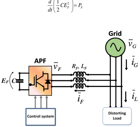
There are mainly two possible configurations, shown in Fig. 1.1. The shunt configuration, Fig. 1.1 (a), is the most used since it can be installed without modifying the plant, as required by the series configuration, Fig. 1.1 (b). It is composed of an inverter connected to the Point of Common Coupling (PCC) through a passive filter.

The inverter can store the electrostatic energy necessary for its operation as electrostatic energy in a capacitor, thus leading to the category of Voltage Source Inverters (VSI) shown in Fig. 1.2(a), or as magnetic energy in an inductor. This solution is referred to as Current Source Inverter (CSI) and it is shown in Fig. 1.2 (b).

(a) (b)

Fig. 1.2. Active Power Filter VSI type (a) and CSI type (b).

(a) (b)

(13)

In this chapter, the operation principles of an APF are discussed and the mathematical model is studied. The control system developed is explained in its part and the reference signal for the current controller, which represents the core of the APF, is derived. The design of the current controller, due to its importance, will be widely studied in Chapter 2.

1.1 M

ATHEMATICAL

M

ODEL OF A

S

HUNT

APF

In this PhD work a VSI type APF, connected through a decoupling inductance, is considered. It is shown in Fig 1.3.

Operation Principles of a Shunt APF

The operation of an APF has to be consistent with the available voltage across the floating capacitor C. The voltage EF of the DC link depends on the electrostatic energy WC stored in

the capacitor 2 1 2 C F W = CE , (1.1)

whose rate of change is related to the instantaneous active power of the converter. If the losses of the APF are neglected, the following expressions can be written:

2 1 2 F F d CE P dt  _{ =}     (1.2)

Grid

APF

G

i

F

i

L Controlsystem

R

_F

, L

_F G

v

F

v

Grid

APF

C

G

i

F

i

L Control system

R

_F

, L

_F G

v

F

v

Distorting Load

E

F

Fig 1.3. Active Power Filter VSI type, connected to the power grid in shunt configuration through a decoupling inductance.

(14)

3 2

F F F

P = v i (1.3)

where PF is the instantaneous active power at the input of the APF, vF and iF are respectively

the space vectors of the output voltage and current of the APF, and "·" is the dot product operator, defined as the sum of the products of the corresponding components of the two vectors.

In order to control the filter current, it is necessary to find the relationship between vF and F

i . In a reference frame aligned with the space vector of the grid voltage v_G, this relationship is given by the equation of the decoupling inductance:

F G F F F F F F di v R i j L i L v dt  = + + + , (1.4)

where ω is the angular frequency of the space vector of the grid voltage vG, RF and LF are

respectively the filter resistance and inductance.

It is straightforward to find the expression of the instantaneous active power PG exchanged

by the grid with the APF through the dot product of (1.4) by 3

2iF: 2 2 3 3 2 4 G F F F F F d P R i L i P dt   = + _ _+   , (1.5) where 3 3 2 2 G G F G Fd P = v  =i v i . (1.6)

In (1.6), iFd is the d-axis component of the filter current i_F, and vG is the magnitude of the

grid voltage vG.

Equation (1.5), combined with (1.2), can be rewritten to emphasize the derivative of the total electromagnetic energy of the system.

2 2 2 1 3 3 2 F 4 F F G 2 F F d CE L i P R i dt  ₊ ₌ ₋     . (1.7)

If the Joule losses of the filter resistance are negligible, (1.7) shows that the rate of change of the energy stored in the reactive elements of the system depends on the instantaneous active power PG, which is proportional to iFd as shown in (1.6). Therefore, the voltage level

(15)

of the DC-link capacitor can be indirectly controlled by adjusting the total energy of the system through iFd, under the assumption that the magnetic energy of the filter inductance is

regarded as a measurable disturbance, which can be properly compensated.

A similar procedure can be used to find the relation between the reactive power exchanged by the power grid and the APF by considering the dot product between (1.4) and 3

2 jiF: 2 3 2 G F F F Q = − L i +Q , (1.8) where 3 2 G G Fq Q = − v i . (1.9)

From (1.8) and (1.9) it can be seen that it is possible to control the reactive power injected into the grid by the APF by acting on the q-component of the filter current iFq and

compensating the reactive power of the decoupling inductance.

With reference to Fig 1.3, if i and _L i_G respectively denote the load and grid current vectors, the balance of the currents at the PCC leads:

F G L

i = − . i i (1.10)

If the high frequency components, identified by the subscript “HF”, are considered, (1.10) allows finding the harmonic content of i_F that nullifies i_{G HF}_, :

, , ,

F HF ref L HF

i = −i . (1.11)

Equation (1.11) states that the shunt APF has to generate the high frequency components of the load current so as to relieve the grid from providing the undesired harmonics.

Since the energy carried by the high-frequency harmonics of the voltages and currents is usually much lower than that of the fundamental components, it results that the low frequency components of the iFd and iFq can be used to control the average energy of the capacitor and

the reactive power at the PCC, according to (1.6) and (1.9), while the high frequency components can be used to reduce the demand of distorted currents of the grid, according to (1.11).

(16)

1.2 C

ONTROL

S

YSTEM

The control system has to:

• provide the inverter with the reference voltages that allow to generate a filter current i_Fnecessary to compensate the power factor and the current harmonics in the power grid;

• maintain control the floating bridge voltage EF at the reference value that

guarantees the correct operation of the APF.

The measurements required by the control system, as shown in Fig 1.4, are: • power grid voltages, used for the synchronization;

• voltage across the floating capacitor;

• filter current iF, which is the one to be controlled, and one current between the

grid and load current. It has been chosen to measure the grid current since it represents the target variable.

Phase Locked Loop (PLL)

The mathematical model has been implemented on a rotating reference frame aligned with the space vector of the power grid voltage, Fig 1.5(a).

Fig 1.5(b) shows the scheme of the PLL. It allows one to estimate the phase angle  that nullifies, instant by instant, the q-component of the fundamental component of the grid voltage. Distorting load PWM d-q α-β F E ref F E , max d i, max d i, − Anti-windup req Fd i , ref Fd i , ref Fq i , Fq i Fd i Ga v Gb v S G v  PLL S ref F v , Notchfilterat the fundamental frequency Notch filter at the fundamental frequency S G i abc ref F v , PI PI abc s -+ Ga i Gb i α-β Ga v Gb v Fa i iFb G i  L i F i abc α-β F E + -+ -Current Controller Distorting load PWM d-q F E ref F E , max d i, max d i, − max d i, max d i, − Anti-windup req Fd i , ref Fd i , ref Fq i , Fq i Fd i Ga v Gb v S G v  PLL S ref F v , Notchfilterat the fundamental frequency Notch filter at the fundamental frequency ref F v , PI PI abc s -+ Ga i Gb i Ga v Gb v Fa i iFb G i  L i F i abc F E + -+ - ΔiF,fond ΔiF,HF S S S F i S L i S G i F F L R , L LL R , α-β α-β α-β abc

(17)

Control of the DC-link

Let us consider the expression of the active power balance (1.7) and develop the derivative: 2 2 3 3 3 2 2 2 F F F F F F G Fd F F C dE E di CE L i v i R i dt R dt   + + = −     . (1.12)

where power loss on the bleeder resistor RC has also been considered.

To find the transfer function of the DC-link voltage loop it is possible to apply small variations to the nominal values as follows:

, , F F nom F Fd Fd nom Fd E E E i i i = +  = +  (1.13)

Substituting (1.13) in (1.12) and under the assumption that iFq =0, following expression

can be written:

(

) (

)

(

)

(

)

(

) (

)

2 , , , 2 , , , , 3 3 2 2 3 2 F nom F F nom F F nom F C G Fd nom Fd F Fd nom Fd Fd nom Fd F Fd nom Fd d E E E E C E E dt R v i i R i i d i i L i i dt  _{+ } _{+ }   _{+ } ₊ ₌     = +  − +  + +  − +  (1.14)

It is possible to neglect the terms of a higher order, such as 2

F E  , 2 Fd i  ,

i

_Fd

d i

Fd

dt



and F F

d E

E

dt



. Equation (1.14) becomes: a) d-q  PLL Gd v abc α-β A v B v α-β Gq v PI 0   ₁ s + + b)

Fig 1.5. Rotating reference frame aligned with the space vector of the grid voltage (a) and control scheme of the PLL (b). O   G v d q G v _ G v _ G Gd v  v t   =

(18)

(

)

₍

₎

(

)

2 , , , , 2 , , , 2 ₃ 2 3 3 2 2 2 F nom F nom F F F nom G Fd nom Fd C Fd

F Fd nom Fd nom Fd F Fd nom

E E E d E CE v i i dt R d i R i i i L i dt +   ₊ ₌ _{+ } ₊  − +  − (1.15)

In addition, by considering the steady state equation 2 2 3 3 2 2 F G Fd F F C E v i R i R = − (1.16)

it is possible to rewrite (1.15) as follows: , , , , 3 3 3 2 2 F nom F Fd F

F nom G Fd F Fd nom Fd F Fd nom

C E E d i d E CE v i R i i L i dt R dt    ₊ ₌ _ ₋ _ ₋ . (1.17)

Expression (1.17) can be written in the Laplace domain as follows

(

)

, , , , 2 3 2 2 F nom

F nom F G F Fd nom F Fd nom Fd

C E sCE E v R i sL i i R   +  = − −        (1.18)

And, finally, the transfer function for the DC-link voltage becomes:

(

)

(

)

(

)

, , 2 1 3 4 1 C G F Fd nom L F DC Fd F nom C R v R i s E G i E s   − ₋  = =  + (1.19) where 2 C C CR  = (1.20) , , 2 F Fd nom L G F Fd nom L i v R i  = − . (1.21)

Equation (1.20) expresses is a time constant related to the floating capacitor, while (1.21) represents a time constant related to the transient of the decoupling inductance to reach the flux value set by the d-component current iFd,nom. It can be noted that (1.19) includes an

unstable real zero, whose sign depends on the sign of iFd,nom, which is related to the condition

of charge or discharge of the floating capacitor voltage. However, the value of τL is much

smaller than τC and describes a fast transient. It is then possible to neglect its contribute for

the DC-link voltage regulation, which can be achieved through a PI controller with an antiwind-up scheme, implemented in the reference frame synchronous with the power grid

(19)

voltage, as shown in Fig 1.4. The reference value of the q-component of the filter current is a degree of freedom that can be used to exchange reactive power with the power grid.

The reference values are then compared with the measurement of the filter current in order to get the input error at the fundamental frequency for the current controller.

High Frequency Current Reference

The input error for the high frequency current is equal to:

, , , ,

F HF F HF ref F HF

i i i

 = − . _(1.22)

By substituting (1.11) in (1.22) and taking into account (1.10) one finds

, ,

F HF G HF

i i

 = − . _(1.23)

The high frequency content of the power grid current is obtained by means of a notch filter at the fundamental frequency. This kind of filter allows one to eliminate a frequency component from a signal. Its transfer function is:

2 2 0 2 2 0 0 2 notch s G s s    + = + + (1.24)

where ω0 is the frequency that should be eliminated and δ is the damping factor. It is possible

to analyze its behavior through the study of the Bode diagram, shown in Fig 1.6, where the magnitude and phase variables are plotted for different values of the damping factor δ.

(20)

A decrease in the value of δ leads to a narrower frequency band around ω0.

The expression for the high frequency input error for the current controller (1.23) can be written as:

( )

, S S F HF notch G

i

G

i



=

−

. (1.25)

where the superscript S means that the variables are written in the stationary reference frame. Equations (1.6), (1.9) and (1.25) define the reference current, in its frequency components, that has to be tracked by the current controller which is studied in the next chapter.

(21)

Chapter 2 C

URRENT

C

ONTROL

Several approaches have been investigated and tested for the current control loop, which, usually, has to track a reference signal composed of several harmonic components. Proportional-integral controllers implemented in a reference frame rotating at the frequency of the disturbing harmonics can be used [3], [4], [5]. Dead-beat and hysteresis controllers [6], [7], [8] require less computational effort than PI controllers implemented in rotating reference frames, but they are not so effective in compensating the harmonic distortion. Recently, repetitive control has been proposed due to its excellent performance in terms of harmonic compensation and low computational burden [9], [10]. Another solution that has become popular in recent years is the use of resonant controllers implemented in the stationary reference frame, or in rotating reference frames, to cancel more harmonic components of the grid current at a time [11], [12]. In [13] several kinds of resonant controllers are compared, such as multiple rotating integrators, stationary frame resonant controllers, proportional-sinusoidal signal integrators and vector PI controllers, in order to determine, for each method, the operating frequency range and the stability limit. A classification of the current control methods is shown in Fig 2.1.

In this PhD work, the methods under investigation are the resonant current control and the repetitive current control.

(22)

2.1 R

ESONANT

C

ONTROLLER

The resonant regulators are able to track sinusoidal references, of direct and inverse sequence simultaneously, with zero steady-state error. They are equivalent to PI regulators implemented in two reference frames having equal and opposite angular frequencies. Their implementation in the stationary reference frame does not require the Park transform, thus allowing a substantial reduction in the computation time. Their use is widespread in power electronics, such as active filters, active rectifiers, wind turbines, hydraulic turbines, inverters for photovoltaic applications, uninterruptible power systems, etc.

Study of the Transfer Function of a Resonant Controller

The transfer function of a Proportional Resonant (PR) controller in the Laplace domain is usually expressed as:

2 2 0 ( ) _p _i s _p _{i R}( ) R s K K K K I s s



= + = + + (2.1)

where Kp e Ki represent the proportional and integral gains respectively, while the function

IR(s) is the resonant term, which has infinite gain at the angular frequency of resonance ±ω0.

The integral gain Ki affects the band width around the resonance peak, and the amplitude of

the resonance peak. The value of Kp defines the gain of R(s) in the remaining part of the

frequency domain. Fig. 2.2 shows the Bode diagram of R(s), with ω0=2π50 rad s-1, Kp

(23)

However, the transfer function in (2.1) is quite sensitive to any mismatch in the resonance frequency and this can be cause of instability, due to the infinite gain. In order to improve the controller robustness, the expression of IR(s) can be modified as follow:

2 2 0 0 ( ) 2 R s I s s



s



= + + (2.2)

where δ is the dumping coefficient, whose increase corresponds to a decrease in the gain at the resonance frequency, as shown in Fig. 2.3.

As the resonance frequency increases the delay introduced by the process of discretization, through the sample and hold, and the delay due to the computation time required by the inverter before generating the output signal, can cause a decrease of the performance or even the instability. It is hence necessary to modify the transfer function (2.2) so as to take into account these delays.

According to [14], it can be rewritten as:

( )

0

( )

2 2 0 0 cos sin ( ) 2 R s I s s s      − = + + (2.3)

where θ represents the delay that affects the regulator. Its value is: 0

C

NT

 =  . (2.4)

The value of N represents the number of sampling periods TS, at the defined resonance

(24)

angular frequency ω0.

For the sake of clarity, it is useful to understand the changes that are brought to (2.3). Let us consider the time domain expression of IR(S) in (2.1) by applying the reverse

Laplace transform

( )

1 0 2 2 0 ( ) cos R s I t L t s   −   = _ _= +   . (2.5)

which represents a sinusoidal signal at the angular frequency of ω0.

Applying the same procedure to the expression of IR(S) one finds:

( )

( ) ( )

(

)

0 1 2 2 0 0 1 1 0 2 2 2 2 0 0 0 0 0 cos sin ( ) 2 cos sin

cos cos sin sin cos

R s I t L s s s L L s s t t t                 − − − −   = _ _= + +       = _ _− _ _= + +     = − = + . (2.6)

which, as expected, gives a sinusoidal signal at the angular frequency of ω0 with initial phase

θ.

It is now possible to write the final form of the proportional-resonant controller as:

( )

0

( )

2 2 0 0 cos sin ( ) 2 p i s R s K K s s      − = + + + . (2.7)

Implemented Multi-Resonant Current Control

The control system developed for the control of the current is composed by an array of proportional-resonant regulators, consisting of a regulator for each harmonic in the set 1,

2, …, N that are intended to be controlled.

As it can be seen in Fig 2.4, the set of resonant controllers can be divided in two parts: • the first part consists in a proportional resonant regulator at the fundamental

frequency, used to control the exchange of active and reactive power,

( )

( )1 ( )1

( )

1 1

( )

1 1 2 2 1 1 1 cos sin 2 p i s R s K K s s       − = + + + ; (2.8)

• the second part is composed of the remaining regulators, whose harmonic order is defined by the letter k, used to compensate the harmonic distortion in the power grid,

(25)

( )

( ) ( )

( )

2 2 2,... 2,... cos sin 2 k k k k k k p i k n k n k k k s R s K K s s       = = −   = _ + _ + +  



. _(2.9)

The reference output voltage collects these two parts multiplied by the respective current input errors as follow:

, 1, ,

2,...,

S S S

F ref F ref Fk ref

k n v v v = = +



_(2.10)

( )

1, 1 , S S S F ref F fond G v = −R s i +v (2.11)

( )

, , 2,..., 2,..., S S Fk ref k F HF k n k n v R s i = = = 



(2.12)

Each resonant controller needs an antiwind-up algorithm. The analysis of the saturation of a multi-frequency regulator is part of this PhD work and it will be widely discussed in the next chapter.

Tuning of the Current Controllers

Let us focus on an example of the tuning of the PR controller of the fundamental component of the current and of the DC-link PI controller, shown in Fig 1.4, that defines the reference iFd. It is necessary to start the analysis from the inner loop, i.e. the current loop,

shown in Fig 2.5. The current open loop transfer function is composed of three terms, which are the PR controller in (2.8), the transfer function of the inverter and the one of the plant

, 1* *

curr ol INV PLANT

G =R G G , _(2.13)

(26)

where 3 2T sS INV G =e− , (2.14) 1 PLANT F F G R L s = + . (2.15)

The value of the sampling time TC is 100 µs, while RF is 26 mΩ and LF is 2,36 mH in the

experimental set-up.

As already mentioned, a PR regulator is equivalent to two PIs implemented in two reference systems rotating at positive and negative speed. It is possible to tune the PR controller by exploiting this equivalence. In particular, it is possible to demonstrate that the gains of the PR regulator can be obtained from those of the PI controllers mentioned above, whose gain values are divided by two.

The integrator of the PI guarantee zero steady-state error, but it also introduces a delay of 90 degrees. This delay is partially compensated by the zero of the PI regulator, which can be placed in cancellation of the pole of the decoupling inductance, i.e. the plant. The only remaining degree of freedom is the integral gain, which can be increased until the phase margin of the open loop transfer function reaches 75 degrees.

This tuning procedure leads to the values for the proportional and integral gains of the equivalent PI controllers, which (divided by two) give the required value for PR regulator

5.2 p K = , _(2.16) 56.5 / i K =  s. (2.17)

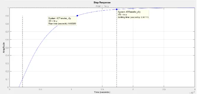
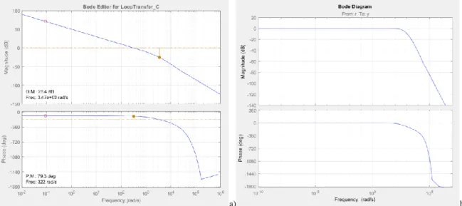
Fig 2.7 (a) and (b) show the Bode diagrams of the transfer function in open loop and in closed loop respectively, with the designed regulator, while in Fig 2.7 the step response of the system is shown.

It is now possible to tune the PI regulator of the DC-link. Let us call ωc the cutting

Fig 2.5Current loop.

R₁ G_INV GPLANT i_Fd,ref i_Fd + -i_Fd

(27)

frequency of the current loop previously tuned, which is equal to 1730 rad/s. The transfer function of the closed current loop can be written as

1 1 curr INV c G G s  = + . (2.18)

With reference to Fig 2.9, the transfer function of the voltage open loop can be expressed as follow: * * F E curr DC G =PI G G , _(2.19) where GDC is given by (1.19).

Fig 2.7Step response of the current closed loop.

a) b)

(28)

With the same procedure used for the tuning of controller R1, the zero of this PI regulator

is placed in cancellation of the pole in (1.19) and the gain increased to a value that guarantees a phase margin higher than 75 degrees. Fig. 2.8 (a) e (b) show the Bode diagrams of the transfer function in open loop and in closed loop respectively, and the step response of the system in Fig. 2.10.

Fig 2.9DC-link voltage loop.

PI GCURR GDC EF,ref EF + -EF a) b)

Fig. 2.8 Bode diagrams of the voltage open loop a) and the voltage closed loop b).

(29)

The study of the stability and tuning of multi-resonant controllers are open topics, given the complexity of these regulators. The choice of the proportional gain Kp is made in such a

way as to have a phase margin that guarantees stability; the optimal number N of delay periods is experimentally found to be equal to 2 [15]; the integral Ki gain and damping δ have

been chosen in such a way as to have a fair compromise between dynamic response and selectivity.

Theoretically the harmonics taken into consideration should be the odd ones until the 19th that are not multiple of three, since the system has three wires. However, due to the presence of single-phase loads connected to the power grid, a third harmonic can be present, making therefore necessary the use of PR regulator for this frequency.

Fig. 2.11 shows the Bode diagrams of the magnitude and phase of the open loop transfer function of Fig 2.5 where the harmonic compensator is also included in this example, the phase margin is 25 degrees.

Discretization of the Control System

In analog systems the input and output signals are continuous functions of time and the mathematical relationships that bind the input to the output are of integral-differential type. The Laplace transform transforms these relations into rational algebraic equations. In order to obtain implementable expressions on a micro-processor, the transform Z is used, which

(30)

allows to pass from the algebraic equations obtained with Laplace transform to numerical iterative equations. The discretization process is fundamental for a resonant regulator, due to the high gain it presents in a narrow band of frequencies. Several discrete-time implementations are possible, but some of these cause discrepancies in resonance peaks compared to what is expected. These inaccuracies can lead to significant performance losses, especially for high-frequency signals. In fact, many of the existing discretization techniques cause a pole shift. This fact translates into a deviation of the resonance frequency and consequently the achievement of a null error is not guaranteed. The error becomes more significant as the sampling period and the resonance frequency increase. Discretization also has an effect on zeros, modifying their distribution with respect to the continuous time transfer function and this has a direct effect on the stability of the system.

The conversion from the Laplace domain to that of the Z-transform can be obtained through the relationships shown in TABLE 1. In [16] an analysis of the performance of

resonant controllers with the different discretization methods has been carried out, highlighting the ones with the best performances in terms of accuracy in the location of the resonant peaks matching of the zeros and poles.

TABLE 1–DISCRETIZATION METHODS

Zero-order Hold 𝑋(𝑧) = (1 − 𝑧−1)𝑍 {𝐿−1₍𝑋(𝑠) 𝑠 )} First-order Hold 𝑋(𝑧) = (𝑧 − 1) 2 2𝑇_𝑐 𝑍 {𝐿 −1₍𝑋(𝑠) 𝑠 )} Forward Euler 𝑠 =𝑧 − 1 𝑇_𝑐 Backward Euler 𝑠 =𝑧 − 1 𝑧𝑇𝑐 Tustin 𝑠 = 𝑧 − 1 (𝑧 + 1) 2 𝑇_𝑐 Tustin con

pre-warping 𝑠 = 𝑧 − 1 (𝑧 + 1) 𝜔₀ tan (𝜔0_{2 )}𝑇𝑐 Zero-Pole matching 𝑧 = 𝑒𝑠𝑇𝑐 Impulse invariant 𝑋(𝑧) = 𝑍 {𝐿−1(𝑋(𝑠) 𝑠 )}

(31)

In this PhD work, among those methods, the one called Tustin with pre-warping has been chosen.

Experimental Results

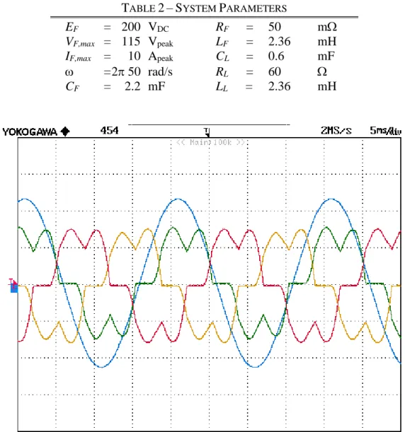
Experimental results have been carried out with a laboratory prototype of a shunt APF, which is used to compensate the highly distorted current produced by a diode bridge feeding a RC impedance, connected to the power grid through a filter inductance. The control system is implemented on a dSpace DS1104 platform and compensates up to the 19th harmonic component of the grid currents. The switching frequency is 10 kHz and the parameters of the experimental system are described in Table 2.

TABLE 2–SYSTEM PARAMETERS

EF = 200 VDC RF = 50 m

VF,max = 115 Vpeak LF = 2.36 mH

IF,max = 10 Apeak CL = 0.6 mF

 =2 50 rad/s RL = 60 

CF = 2.2 mF LL = 2.36 mH

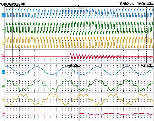
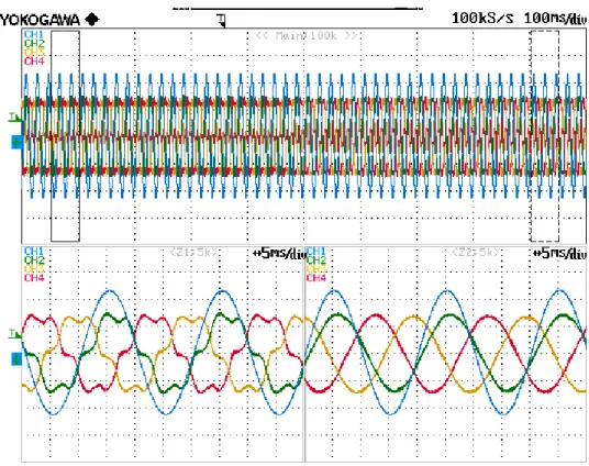
Fig. 2.12 Waveform of the grid currents and fundamental component of the phase voltage when the APF is off. Scale: current (2 A/div), voltage (40 V/div)

(32)

Without any compensation, the currents absorbed by the passive load are the ones shown in Fig. 2.12. The phase delay of the phase current and the phase voltage is due to the decoupling inductance through which the distorting load is connected to the grid. The perfect sinusoidal waveform of the phase voltage is due to a software filter that extracts the fundamental component used for the synchronization of the PLL.

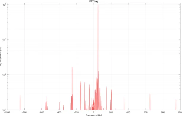
In Fig. 2.14 the spectrum of the grid current of Fig. 2.12 is shown in semi-logarithmic scale and normalized to the fundamental component. This spectrum is evaluated over a 1kHz band, which is wide enough to assess the most prominent current harmonics. The highest current harmonics are the fifth harmonic of the inverse sequence and the seventh harmonic of the direct sequence. Also, it can be noticed that a first inverse harmonic as well as a third direct harmonic are present. They

are caused by the imbalance of the three currents of network. For this harmonic spectrum, the THDI is 21,56%.

As the APF turns on the DC-link control loop brings the voltage of the floating capacitor from the phase-to-phase peak voltage of 150 V to the reference value of 200 V as shown in Fig. 2.13.

Fig. 2.14 Normalized spectrum of the grid currents when the APF is off.

Fig. 2.13 Transient of the floating bridge voltage to the reference value. Scale: voltage (100 V/div)

(33)

Fig. 2.16 Transient of the power grid currents due to the charge of the DC-link. Scale: current (2 A/div), voltage (40 V/div)

Fig. 2.15 Transient due to the charge of the DC-link of the power grid phase voltage and current, load current and filter current. Scale: current (2 A/div), voltage (40 V/div)

(34)

Fig. 2.15 shows the transient of the grid voltage and current, load current and filter current due to the charge of the DC-link. The PI controller that regulates the floating capacitor voltage provides the reference value for the d-component of the filter current. The resonant controller at the fundamental frequency tracks the reference value of the current, which causes an increase in the active power absorbed by the APF in order to increase its DC-link voltage, hence an increase in the current coming from the power grid. In Fig. 2.16 the same transient is shown and the behavior of the power grid current is highlighted.

Fig. 2.17 shows transient of the power grid phase voltage and current, load current and filter current due to the activation of the harmonic compensation.

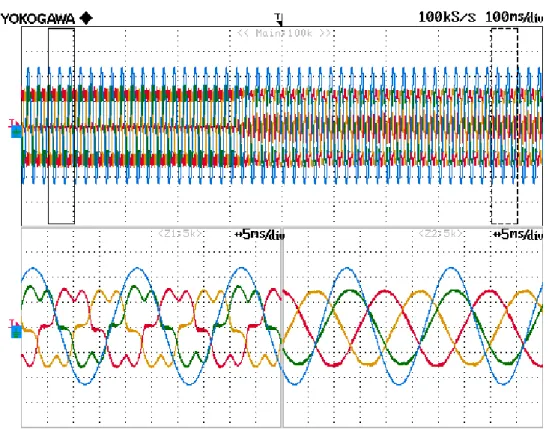
In Fig. 2.18 the steady-state waveform of the power grid currents is shown and their harmonic spectrum is represented in Fig. 2.19. The THD of the power grid currents when the APF is tuned on drops to the value of 2,60%, proving therefore the good performance of the developed control system.

Fig. 2.17 Transient of the power grid phase voltage and current, load current and filter current due to the activation of the harmonic compensation. Scale: current (2 A/div), voltage (40 V/div)

(35)

It is possible to notice in Fig. 2.18 that there is a delay of the power grid current to the power grid phase voltage. It is possible to compensate the reactive power of the grid by acting on the q-component of the filter current at the fundamental frequency. The results of the reactive power compensation are shown in Fig. 2.20.

Fig. 2.19 Normalized spectrum of the grid currents when the APF is on.

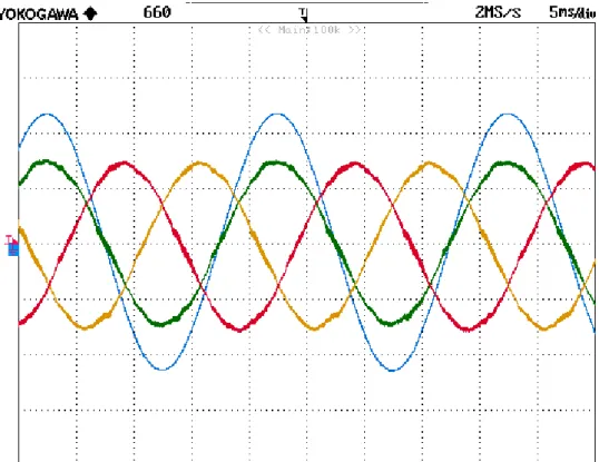
Fig. 2.18 Power grid currents before and after the harmonic compensation of the APF. Scale: current (2 A/div), voltage (40 V/div)

(36)

Fig. 2.20 Reactive power compensation of the power grid through the APF. Scale: current (2 A/div), voltage (40 V/div)

(37)

2.2 R

EPETITIVE

C

ONTROLLER

Relation between Resonant Controller and Repetitive Controller

The relation between resonant and repetitive controllers (RCs) has been object of study in the literature of the last decade [17]- [18]. Both are based on the Internal Model Principle (IPM), which affirms that a sufficient condition for the asymptotic tracking of the reference signal is that the transfer function obtained by merging the controller and the controlled plant contains the generating polynomial of the reference signal in the denominator.

Let us then consider a sinusoidal reference signal with angular frequency equal to kω0,

where ω0 is considered as fundamental component and k represents the harmonic order,

written in the Laplace domain:

(

)

(

)

0 ₂ 2 0 ( ) cos ref s I s L k t s k   = _ _= + (2.20)

which is equal to the transfer function of a resonant controller with frequency kω0. Thanks to

the IPM, the resonant controller at kω0 is able to track a sinusoidal signal at that frequency.

If the reference signal is composed by the sum of N sinusoidal signals at multiple frequency of the fundamental one,

(

0

)

0 ( ) cos N ref k I t kt = =



(2.21)

then the controller able to track it, has to have the sum of N resonant controllers, one for each sinusoidal signal that contributes to the reference signal, as follow:

(

)

2 2 0 ₀ N i k s K s k = +



. _(2.22)

If the number N of resonant controllers summed up in (2.22) tends to infinite, for the properties of the exponential functions, it can be written:

(

)

0 0 0 0 2 2 0 ₀ 0 s s i i s s k s e e K K s k e e            −  − =   +   = _ _ + _ _ −  



(2.23)

which, with few mathematical steps and by neglecting for the moment the gain in front of the transfer function, can be written as follow:

(38)

0 0 1 1 sT RC sT e G e − − + = − . (2.24)

The (2.24) represents the transfer function of a repetitive controller, whose control scheme is shown in Fig 2.21.

It sums to the input reference, the same signal delayed of a period T0. This cause an infinite

number of resonances at multiple frequencies of the fundamental one f0 =1/T0, as can be

found by nullifying the denominator of (2.24):

0 0 0 0 0 0 1 1 1 cos( ) sin( ) 0 2 sT j T res e e T j T T k f kf k  _ _   − − − = − = − + =   =  =  (2.25)

(2.25) confirms hence that the repetitive controller is equivalent to a sum of infinite resonant controllers. These resonances, obtained by buffering the reference input signal, imply a lower computational burden compared with the resonant controllers, but it requires a memory effort in order to store a whole period of the input signal.

The feedforward contribute instead, causes an infinite number of zeroes in (2.24), located in between the resonance frequencies, as shown in (2.26).

(

)

(

)

(

)

0 0 0 0 0 0 1 1 1 cos sin 0 1 2 1 , , 2 sT s j j T zeros e e T j T T k f k f k   _ _   − = − + ⎯⎯⎯→ + = + − =     = +  =_ + _    (2.26)

The Bode diagrams of the magnitude and phase for the transfer function (2.24), are represented in Fig. 2.22.

A simpler version of repetitive control can be obtained if the control scheme shown in Fig 2.21 is modified by cutting away the feedforward path as shown in Fig. 2.23(a).

Fig 2.21. Repetitive control scheme. +

+

𝑒−𝑠𝑇

Δi + v

(39)

As already said during the study of the resonant controller, it is necessary to take into account the delay introduced by the process of discretization and compensate it with a phase lead. If Td represents this phase delay, the scheme Fig. 2.23(a) can be modified as shown in

Fig. 2.23(b), which transfer function can be found with the following mathematical steps:

(

)

( ) (0 ) 0 0 0 0 1 1 d d d d s T T sT s T T sT sT sT sT e e v i ve e i e i e e − − − − − − − − =  + =  =   − − (2.27) 0 0 (1) 1 d sT sT FHRC sT e G e e − −  = − . (2.28)

The transfer function (2.28) still presents the same resonance frequencies of (2.24), ensuring the harmonics tracking, and the delay on the direct path allows one to achieve also a phase lead, which is causal as long as T_d T₀.

This topology will be indicated with the superscript (1) hereafter, while the subscript

Fig. 2.22 Bode diagrams of the repetitive controller base scheme.

a) b)

Fig. 2.23 Base scheme of a repetitive controller a) and base scheme with the phase lead b +

+ 𝑒

−𝑠𝑇

(40)

(FHRC) stands for “Full Harmonic Repetitive Controller” and will be used for those configurations that presents resonance frequencies for all the multiple frequencies of the fundamental one.

The Bode diagrams of magnitude and phase for the transfer function in (2.28) are shown in Fig. 2.24.

Taking into account the delay compensation of Td for the control scheme of Fig 2.21 is

not as easy as for the topology 1, due to the fact that the delayed period T0 is not on the direct

path.

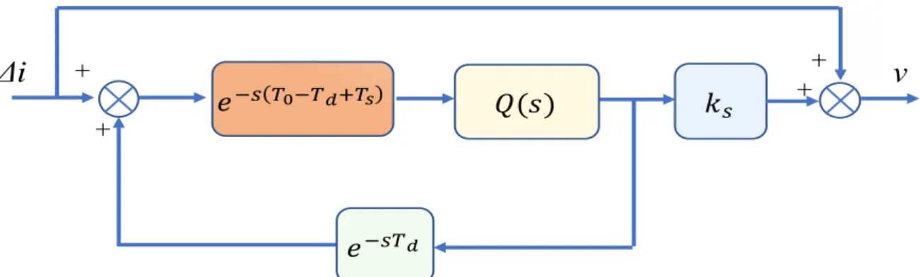
The phase lead has been achieved by adding a further period delay from which the phase lead is obtained. The term is represented by the function 𝑒−𝑠(𝑇−𝑇𝑑)_{in the control scheme of}

Fig. 2.24 Bode diagrams of the base scheme transfer function 𝐺_{𝐹𝐻𝑅𝐶}(1) .

Fig 2.25. Repetitive control scheme – Topology 2, FHRC. + + 𝑒−𝑠𝑇 Δi v 𝑒−𝑠 𝑇−𝑇𝑑 + +

(41)

Fig 2.25. The transfer function modifies as follow: ( ) 0 ( ) 0 0 2 1 1 d sT s T T FHRC s sT e G k e e − − − − + = − . (2.29)

Stabilization of the Repetitive Control

The high gain over a wide frequency band affects the system stability. Several solutions have been investigated in order to stabilize this kind of controllers. An interesting solution has been developed in [19], where a low pass filter with zero-phase shift has been used to reduce the contribution at high frequency of the repetitive controller. The general expression of a zero-phase filter can be written as follow:

lim lim 0 1 1 ( ) n n sn sn n n n n Q s C e−  C C e  = = =



+ +



, (2.30)

Whose first order approximation is:

( )

lim lim 0 1 0 1 1 1 1 1 0 ( ) 2 2 cosh 2 n n sn sn s s n n n n s s Q s C e C C e C e C C e e e C C s C        − − = = − = + + + + = + = = +



(2.31)

The values for the coefficients C1 and C0 can be found by writing (2.31) in the domain of

the angular frequency ω,

(

)

( )

1 0 1 0

( ) 2 cosh 2 cos

Q  = C j +C = C  +C . (2.32)

In order to have 0Q

( )

 1, the constraint of the coefficient becomes:

0 1

0C +2C 1 (2.33)

Equation (2.32) represents a real number, which behaves as a moving average low-pass filter variable with the frequency. Its magnitude has a minimum for

 

= . The frequency of this minimum can be found as:

min 1 2 f  = . (2.34)

Choosing τ = 𝑇s, where 𝑇s represents the sampling period, sets the system Shannon

frequency as the frequency for which the filter has a minimum, obtaining a decreasing trend in the whole system band. In Fig 2.27 the trend of the gain of the filter is shown when its

(42)

coefficients vary; the sampling frequency has been assumed to be 10 kHz, so the trend of the module up to 5 kHz is shown.

The cut-off frequency decreases as C1 increases. It is important to design this filter with a

cut-off frequency above 1 kHz, where the harmonics of interest are, in order to not interfere with the current controller. The filter Q(s) strongly reduces high frequencies disturbances, which may be harmful and cause of instability.

However, this filter topology is not implementable due to the lead phase term C1 esτ in its

transfer function. Nevertheless, once again, it is possible to compensate the phase lead required by the filter by including it in the direct path, where it is multiplied by a delay operator. It is possible to write:

(

)

2 1 0 1 1 0 1 ( ) ( ) sTs sTs sTs sTs s Ts sTs Q s =Q s e− = C e− +C +C e e− =C e− +C e +C , _(2.35) (0 ) 0 ( ) sT ( ) s T Ts Q s e − =Q s e− + . (2.36)

Fig 2.27. Bode diagram of the magnitude of the average moving low pass filter

0.6

frequency

Fig 2.26. Repetitive control scheme implemented – Topology 1, FHRC.

𝑒−𝑠 𝑇 −𝑇𝑑 𝑇

Δi

v

𝑒−𝑠𝑇𝑑 (𝑠) + + 𝑠 + +

(43)

The control scheme of the repetitive controller of Fig. 2.23(b) can be implemented as shown in Fig 2.26. Its transfer function is:

( )

( ) ( ) 0 0 1 1 , 1 1 1 s d s s T T sT FHRC plug in s s T T FHRC Q s e G k e G Q s e − + − = ₋ − + + = + . (2.37)

In addition to the filter Q(s), a series gain ks has also been added. It is used to increase the

controller gain overall the bandwidth.

A “plug-in” path is added to control scheme of Fig 2.26. It sums the input error to the repetitive output and allows one to define a regulation loop that does not include the controller. This feature will helpful in the mathematical steps for the tuning of the series gain ks.

Likewise (2.28), the repetitive controller 𝐺_{𝐹𝐻𝑅𝐶}(1) contains resonance frequencies for all the multiple harmonics of the fundamental one.

The tuning of the series gain ks is accomplished by studying the stability of the

closed-loop (2.38), shown in Fig 2.28.

( )

(

)

( )

(

)

( )

_{( )}

(

)

(

)

( )

_{( )}

(

_{( )}

)

0 0 1 , ₁ 1 1 1 1 1 1 1 d d d d s T T sT s FHRC INV PLANT current cl s T T sT s FHRC INV PLANT e Q s k e G s G G G G e Q s k e G s G G G − − − − − − + = = − − + + . (2.38)

According to [19], the current loop is stable if: • the transfer function (2.39), considering 𝐺_{𝐹𝐻𝑅𝐶}(1)

= 0, is stable, 1 INV PLANT INV PLANT G G G G G = + (2.39)

• the denominator of (2.38) is not zero in the frequency band up to the Shannon

Fig 2.28. Current control loop.

G_RC G_INV G_PLANT + + +

(44)

frequency 2 s f ,

( )

(

1 sTd

( )

)

1 s Q s −k e G s  . (2.40)

By writing (2.40) in the frequency domain and Q and G in polar coordinates, the last condition becomes

( )

(

_{( )}

( ( ) )

)

( )

( ( ) )

(

)

_{( )}

1 1 1 1 Q G d G d j j T s j T s Q e k G e k G e Q             + + −    −  (2.41)

By solving the last inequality, one finds the values of the series gain ks that satisfy the

stability condition,

( )

(

)

( )

2 2 2 1 2 cos 0 _s G d s Q T k G Q k G        − +   + . _(2.42)

The last condition can be approximated since the first term of upper limit tends to zero in the frequency band of the regulator, becoming:

( )

(

)

( )

2 cos 0 k_s G Td G     +   . _(2.43)

It can be noticed that there are admissible values of ks as long as

( )

2

G Td

   +  . It is then possible to choose the phase Td in order to maximize the upper bound of the series gain.

In Fig 2.29 is shown the trend of the series gain ks for different values of the phase lead

Fig 2.29. Trend of the series gain ks for different value of the phase lead Td.

Td=2Ts

frequency

Td=3Ts

(45)

Td, which depends on the number of sample time that have to be compensated.

The Bode diagrams of magnitude and phase of 𝐺_{𝐹𝐻𝑅𝐶}(1) in (2.37) with the low-pass filter and the series gain so tuned become as shown in Fig. 2.30

Similar techniques are used to stabilize the topology of repetitive controller shown in Fig 2.25, which modifies as shown in Fig 2.31.

The transfer function for this control scheme becomes:

Fig. 2.30 Bode diagrams of the transfer function 𝐺_{𝐹𝐻𝑅𝐶}(1) stabilized.

Fig 2.31. Repetitive control scheme implemented – Topology 2, FHRC.

+ +

𝑒

−𝑠 𝑇 𝑇

Δi

v

𝑒

−𝑠 𝑇−𝑇𝑑 + + 𝑠

(𝑠)

+ +

(46)

( )

( ) ( ) ( ) 0 0 0 2 2 , 1 1 1 1 s d s s T T s T T FHRC plug in s s T T FHRC Q s e G k e G Q s e − + − − − − + + = + = + − . (2.44)

The tuning of the gain series gives the following range of admissible values:

( )

(

)

( )

(

( )

)

2 1 2 2 2 * * 1 2 cos 2 cos 0 s s Q k G k G k Q Q k G           −   + + . _(2.45)

where the parameters k*, θ1, θ2 and θ3 stand for:

( )

(

( )

)

( )

(

( )

)

* 3 1 1 1 1 cos _Q 1 1 cos k G    Q  Q            =_ + + _ +  _{ }+ − _ _       , _(2.46) 1 G Td  = + , (2.47) 2 G Td Q  = + − , _(2.48) 3 1 2  = + . (2.49)

The Bode diagrams of magnitude and phase of (2.44) are shown in Fig. 2.32.

(47)

Odds Harmonic Repetitive Controller (ODRC)

It is possible to change the set of resonance frequencies for both topologies shown, by acting on the sign of the feedback signal. The control scheme of Fig 2.26, modified as shown in Fig 2.33, has the following transfer function

( )

( ) 0 0 2 1 1 , 2 1 1 1 s d s T s T sT

ODRC plug in s T OHRC

s T Q s e G k e G Q s e   −_ + _   − ₋ ₊      = − + = + + . _(2.50)

The set of resonance frequencies can be found equating to zero the denominator of 𝐺_{𝑂𝐷𝑅𝐶}(1) ,

(

)

(

)

0 0 0 2 0 0 1 1 cos sin 0 2 2 2 1 2 1 , , 2 T j res T T e j T k f k f k      −     + = + _ _− _ _=       = +  = +  (2.51)

The resonance frequencies are located at the odd harmonics of the fundamental frequency f0.

The Bode diagrams of 𝐺_{𝑂𝐷𝑅𝐶}(1) , without considering the effects of Q(s) and ks, are shown in

Fig 2.33, while in Fig. 2.35 the same diagrams are shown after the stabilization procedure.

Fig 2.33. Repetitive control scheme implemented – Topology 1, ODRC.

𝑒

−𝑠 𝑇2 −𝑇𝑑 𝑇

Δi

v

𝑒

−𝑠𝑇𝑑

(𝑠)

+ + 𝑠

(48)

-Fig. 2.34 Bode diagrams of the transfer function 𝐺_{𝑂𝐻𝑅𝐶}(1) not stabilized

Development of Grid-Connected and Front-End Converters for Renewable Energy Systems and Electric Mobility

DOTTORATO

DI

RICERCA

IN

Ingegneria Biomedica, Elettrica e dei Sistemi

Ciclo XXXI

TITOLO TESI