PSO-Based Real-Time Control of Planar Uniform Circular Arrays

UNIVERSITY

OF TRENTO

DIPARTIMENTO DI INGEGNERIA E SCIENZA DELL’INFORMAZIONE

38123 Povo – Trento (Italy), Via Sommarive 14

http://www.disi.unitn.it

PSO-BASED REAL-TIME CONTROL OF PLANAR UNIFORM

CIRCULAR ARRAYS

M. Benedetti, R. Azaro, D. Franceschini, and A. Massa

January 2011

1

PSO-Based Real-Time Control of Planar

Uniform Circular Arrays

Manuel Benedetti, Renzo Azaro, Davide Franceschini, and Andrea Massa1

Abstract—This paper is aimed at assessing the effectiveness of the phase-only control strategy based on a customized PSO when applied to planar uniform circular arrays (PUCA) and in the presence of interferences both in the near-field and far-field of the antenna. The employed geometry seems to be suitable for a reliable and effective implementation of adaptive arrays in mobile devices thanks to its symmetry and geometric simplicity. For validation purposes, the proposed architecture is evaluated in the presence of a complex time-varying scenario both in terms of synthesized beam patterns and signal-to-interference-plus-noise ratio.

Index Terms—Circular Arrays, Adaptive Control, Particle Swarm Optimizer, Phased Array, Smart Antennas.

I. INTRODUCTION

The adaptive control of array antennas is a topic of growing interest because of the continuous development of communication systems and related services. In fact, the pervasive employment of mobile devices requires suitable control methods able to take into account the changing environment conditions for allowing an efficient exploitation of the communication channel. Within such a framework, smart antennas play a key-role because of their capacity of rejecting undesired signals thus enhancing the quality of the service at the receiver [1].

In the literature, many efforts have been addressed to the development of efficient control techniques for properly tuning the weight coefficients of adaptive arrays starting from a widely used model [2]. Moreover, the possibility of reducing the computational costs has been deeply investigated recurring to phased arrays [3].

However, even though the impact of control methodologies has been carefully analyzed and effective solutions proposed, the choice of array geometries as well as their integration in the whole smart system architecture has been only partially discussed. As a matter of fact, a large set of control strategies have been evaluated especially dealing with linear and rectangular arrays, but the use of different topologies could enhance the well known potentialities of control methods. For instance, uniform circular arrays (UCA) allow the electronic steering of the main lobe towards the direction of the desired signal without penalizing the beam pattern shape in other directions [4]. Moreover, adaptive hybrid structures as the planar UCA (PUCA) profitably exploit the potentialities of rejecting jamming signals with the ability to scan a beam azimuthally through the whole angular range maintaining either the beamwidth or the side lobe level.

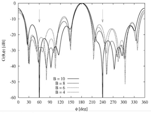
Fig. 1. Samples of synthesized beam patterns by varying B (Scenario #1).

For these reasons, this work is aimed at numerically assessing the implementation of an effective real-time phase-only control

The authors are with ELEDIA Group at the Department of Information and Communication Technology, University of Trento, Via Sommarive 14, 38050 Trento, ITALY (phone: +39 0461 882057; fax: +39 0461 882093; E-mail: andrea.massa@ing.unitn.it and {manuel.benedetti, renzo.azaro, davide.franceschini}@dit.unitn.it; Web-site: http://www.eledia.ing.unitn.it).

This work was in part supported in Italy by "Study and Developement of Innovative Smart Systems for Higly Reconfigurable Mobile Networks", Progetto di Ricerca di Interesse Nazionale - Miur Project COFIN 2005099984_001

when both near-field and far-field interferences with random directions of arrival (DoAs) are present, thus extending the analysis carried out in [4].

II. MATHEMATICAL FORMULATION

Let us consider a PUCA of N elements organized in M concentric circular rings

∑ ∑

= = = M m N n m m m n N 1 1 (1)

where the index m ( ) indicates the m-th concentric ring ( in radius) of the array, identifies the generic element of the m-th ring, and denotes the number of elements of each ring.

M

m=1,..., r_m

n

m

m

N

Accordingly, a generic signal received at the n_m-th element of the array turns out to be

{ }

() ) ( ) ( exp ) ( ) ( nr r r nm t t j m s =α ϕ (2) where and are the envelope and the phase of the received signal, respectively. Under the assumption of far-field conditions [8], is given by ) (r α (r) nm ϕ ) (r nm ϕ

(

m

)

m n r r m r n _λ r θ φ φ π ϕ()= () ()− cos sin 2 ₍₃₎

(

m m nm π n N

)

φ =2 being the angular position of the nm-th element of the array.

Scenario #1 #2 Desired

(

( ) ( )

)

, d d _φ θ (π_,π) 2

(

π

)

π_, 2 DoAs Interferences

(

() ()

)

, i j i j φ θ j = 1;

( )

3 2, π π j = 2;

(

4₃

)

2, π π j = 1;

( )

π₂,π₆ j = 2;

(

2₃

)

2, π π j = 3;

(

5₃

)

2, π π

Tab. 1. Descriptions of the environmental scenarios.

As far as the environment scenario is concerned, the received signal (r) is the result of different contributions due to the desired signal (d), a set of j=1,_K,J interference sources (i), and a background noise η . By considering general conditions where jamming sources are located both in the far-field and near-field of the radiating zone of the array, the DoA of the jth jamming source is no longer defined only in terms of the angular coordinates

(

()_, (i)

)

j i j φ

θ , but also through the distance of the interferer. Consequently, as suggested in [9], the phase term of the j-th jammer is equal to

) (i j d

(

)

_⎥⎦⎤ ⎢⎣ ⎡ _{− + − +} = () ()2 () () () 2 ) ( , 2 sin cos 2 m n i j i j i j m i j i j i j nm λ d d rd θ φ φm r π ϕ (4) J j=1,_K, ; m=1,_K,M; nm=1,K,Nm.

Taking into account these conditions and the PUCA geometry, the control problem is then recast as the maximization of the signal-plus-interference-to-noise ratio (SINR) at the receiver through the optimization of the fitness function [10]

( )

(

)

w w w w _{T r} d d T ) ( ) ( ) ( , Ψ Θ = Γ θ φ (5)

with respect to the phase components of the coefficients vector

( )

{

T m m n n j n N m M w w= _mexp β_m; =1,..., ; =1,...,

}

(6)

3 m n w and m n

β

being the amplitude and phase of the nm-th element, respectively. Moreover,

) (r

Ψ is the covariance matrix of the received signal (r) measurable at the receiver and

(

( ) ( )

)

, d

d φ θ

Θ is a vector whose n_m-th term is given by

(

m m

)

m m n d n m d d n

_λ

u r

φ

v r

φ

π

sin cos 2 ( ) ( ) ) ( = +

Θ being u(d) =sin

θ

(d)cos

φ

(d) and v(d) =sin

θ

(d)sin

φ

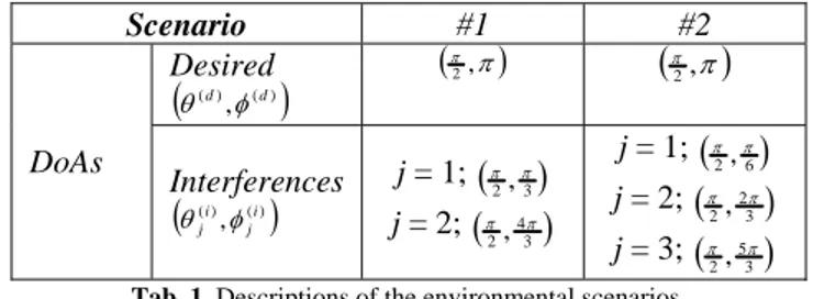
(d).

Fig. 2. Comparative Assessment (Scenario #1) – Beam patterns synthesized with different control techniques.

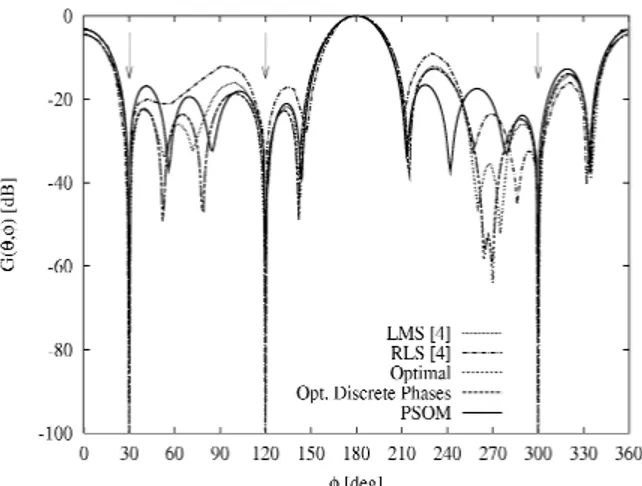
Fig. 3. Comparative Assessment (Scenario #2) – Beam patterns synthesized with different control techniques.

As far as the optimization strategy is concerned, the particle swarm optimizer with memory (PSOM) [7] is adopted. A swarm of S binary-coded trial solutions (B being the number of bits used for coding

m n

β

) is defined

[ ]

(

)

{

b B nm Nm m M

}

k n s b k s l m l ,..., 1 ; ,..., 1 ; ,..., 1 ; 1 , 0 1 , , ∈ = = = Φ = Φ + ₍₇₎

kl ( ) denoting the generic iteration of the optimization process carried out at the time-step , and it evolves by

updating each component of the particles positions with a velocity

max K k_l ≤ t_l

(

)

{

(

)

m l m l m l m l m l m l m n b k n s b k n s b k n s b k n s b k n s b w k n s b A r c r c r c i , 3 3 , , , , 2 2 , , , , 1 1 , , 1 , , + Φ − + + Φ − + Λ = + ς ξ ν ν

}

(8) where:

• i_w is the inertial weight [6];

• c_q and r_q (q=1,K,3) are constant weighting parameters and uniformly-distributed random variables, respectively [5];

•

{

[

( )

l

]

}

l l l h s k h k s =argmax =1,K, ΓΦ

ξ is the s-th particle “personal best” position; • l

{

[

( )

kl

]

}

s s p k s ξ

ς =argmax =1,K, Γ is the swarm “global best” position; • Λ is a threshold function [7];

[

(

)

]

Q H A Q q Q q n q b n b m m

∑

= − − = 1 1 , , , exp ς , (9)

which depends on the sub-set of Q trial solutions

{

q Q

}

q; =1,...,

ς stored in a buffer of size Q, (i.e., the “swarm memory”) and H is a coefficient heuristically chosen [7].

Concerning the “memory” mechanism, an exchange of trial solutions between the swarm and its memory is performed by means of the “Resurrection Operator” and the “Storage Operator” [11] during the sequence of time-steps, , t_l l=1,...,L_max.

I. NUMERICAL ANALYSIS

In this section, a selected set of numerical results are discussed in order to summarize the assessment of the PSOM-based approach when applied to PUCA and in correspondence with a complex scenario.

The first example deals with a PUCA characterized by N =16 isotropic elements arranged as that analyzed in [4] (M =2, -

6

1=

N r₁=3

λ

/2

π

, N₂=10 - r₂=5

λ

/2

π

). The same interference “static” configuration #1 described in Tab. I have been assumed, as well, for comparison purposes.

As far as the array control technique is concerned, uniform array amplitudes =1.0 m

n

w have been assumed and the quiescent pattern (i.e., without jammers) has been computed by setting the phase terms

m

n

β

for steering the main lobe of the array towards the DoA of the desired signal. Moreover, since the scenario is not time-varying, the “memory” mechanism has been disabled by setting . The other PSOM parameters have been heuristically chosen according to the results of a calibration procedure. More in detail, the values of and have been set to 2.0 according to [5], while has been assumed equal to 0.01 in order to favor the reaction and adaptability of the control method to environmental changes thus improving the convergence rate ( ). Furthermore, the size of the swarm (S = 30) and dimension of the memory buffer (Q = 20) has been selected for allowing a good trade-off between convergence rate and effectiveness of the adaptive control.

0 . 0 3= c 1 c c2 iw 100 max = K

As an example of the calibration of the PSOM-based control, Figure 1 shows the samples at _θ=π_{2of the beam pattern}

( )

(

)

[

]

N r j w G M m n m N n n m m m m

∑∑

= ⎪⎭ ⎪ ⎬ ⎫ ⎪⎩ ⎪ ⎨ ⎧ − = 1 cos sin 2 exp , λ φ φ θ π φ θ (10) determined at the end of the optimization process for different quantization values (B) of the phase terms. The optimal value both in terms of interference rejection capacity and computational costs turned out to be B=10 and this value has been adopted in the following.

For a comparative analysis, the result obtained with the PSOM has been compared with that from the reference Applebaum’s method [2], the Applebaum’s method with quantized values of the phase coefficients, the LMS technique, and the RLS method [4]. The optimization processes have been carried out by setting the power of the interferers to 30 dB with respect to the power level of the desired signal and by neglecting the background noise [4]. The results are shown in Fig. 2 in terms of convergence beam patterns. As it can be observed, the PSOM-based control was able to place nulls with depth G

( )

π₂,π₃ =−71 dB and

(

, 3

)

68

4

2 =−

π π

G dB in the direction of interference sources obtaining lower secondary lobes than that of LMS and RLS despite no side-lobe level constrains have been imposed.

The same considerations hold true also for the configuration #2 in Tab. I (the power levels of the configuration #1 are adopted). As a matter of fact, suitable nulls are located in correspondence with the jammers directions [

( )

2,6 =−70

π π G dB,

(

,2₆

)

57 2 =− π π

5

Fig. 4. Complex Interference Scenario – Plot of the number of jammers vs. time-step index.

The second test case is concerned with a more complex and now time-varying scenario. Towards this end, a sequence of time-steps has been considered characterized by a random and different number of impinging jammers as shown in Fig. 4. The arrival time of each interferer has been modeled through a Poisson random process [12] with

100 max = L 1 = λ and a maximum life-time of 5 time-steps.

In order to properly deal with such a scenario, the “memory” mechanism of the PSOM has been enabled setting c3=1.0 and .

10 =

H

Fig. 5. Comparative Study (Complex Interference Scenario) – Running average of the SINR vs. time-step index.

As far as the DoAs of the J jammers are concerned, each angle of incidence was a random variable φ(ji)∈

[

0,2π

]

uniformly distributed, with θ(i) _=π2

j . Moreover, the distance of the jamming sources has been modeled as a random variable

uniformly distributed between 3λ and 100λ.

) (i

j

d

to deal with more realistic conditions, a background noise of -30 dB has been also added.

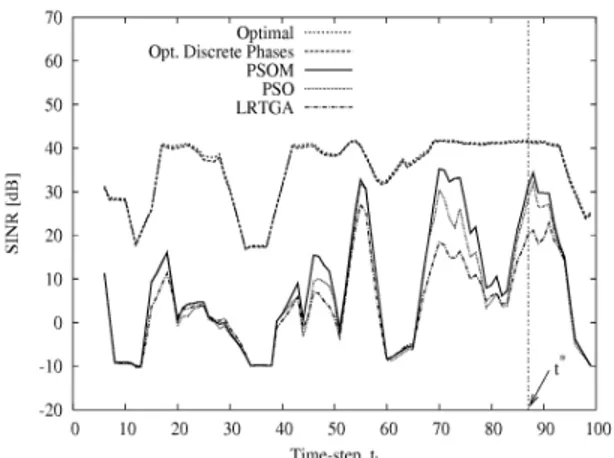
As a representative sample of the obtained results, Figure 5 shows the SINR averaged over a sliding window of Δt_l =5 time-steps for different control techniques. In particular, the PSOM has been compared with the optimal technique [2], the standard

PSO implementation [7], and the Learned Real-Time Genetic Algorithm (LRTGA) [11]. In order to achieve the same time of

response at each time-step, the values of of PSO and LRTGA have been set to 100 and 25, respectively. As a matter of fact, the computational burden of PSO is equal to that of the PSOM, while LRTGA is about 4 times heavier.

max

K

As it can be noticed, the result achieved by the proposed technique overcomes the performances of both the LRTGA and the

PSO, thanks to the “ambient-knowledge” and the exploitation of the “memory” of the system.

Finally, Figure 6 shows the shape of the beam pattern in correspondence with a time-step (l = 87) of the time-varying evolution of the environmental scenario. In such a case, four interferences impinge on the receiver. Three jammers are grouped into a cluster near φ(i) ₌11_6π

j , whereas the other hits the array from a direction close to the main lobe. As expected, the

PSOM-based method effectively rejects the interferers by properly placing the beam pattern nulls in the DoAs of the jammers.

II. CONCLUSIONS

In this letter, the application of an efficient beamforming strategy to planar uniform circular arrays has been considered. After a brief description of the implementation of the PSOM control strategy in circular geometries and some details on the calibration of the approach, the achieved performances both for static and time-varying configurations have been compared with those of state-of-the-art techniques showing its effectiveness in rejecting interferences and pointing out the potentialities of the whole architecture.

REFERENCES

[1] M. Chryssomallis, “Smart Antennas,” IEEE Antennas Propagat. Mag., vol. 42, no. 3, pp. 129-136, Jun. 2000. [2] S. P. Applebaum, “Adaptive Arrays,” IEEE Trans. Antennas Propagat., vol. 24, pp. 585-598, Sep. 1976.

[3] R. L. Haupt, “Phase-only adaptive nulling with a genetic algorithm,” IEEE Trans. Antennas Propagat., vol. 45, pp. 1009-1015, Jun. 1997.

[4] P. Ioannides and C.A. Balanis, “Uniform Circular and Rectangular Arrays for Adaptive Beamforming Applications,” IEEE Antennas and Wireless

Propagation Letters, vol. 4, pp. 351-354, 2005.

[5] J. Robinson and Y. Rahmat-Samii, “Particle swarm optimization in electromagnetics,” IEEE Trans. Antennas Propagat., vol. 52, no. 2, pp. 397-407, Feb. 2004.

[6] R. Eberhart and J. Kennedy, “A new optimizer using particle swarm theory,” Proc. Sixth Int. Symp. Micro-Machine and Human Science (Nagoya, Japan), pp. 39-43, 1995.

[7] M. Donelli, R. Azaro, F. De Natale, and A. Massa, “An Innovative Computational Approach Based on a Particle Swarm Strategy for Adaptive Phased-Arrays Control,” IEEE Trans. Antennas Propagat., vol. 54, no. 3, pp. 888-898, Mar. 2006.

[8] C. A. Balanis, Antenna Theory. New York: Wiley, 1996.

[9] A.J. Fenn, “Evaluation of adaptive phased array antenna far-field nulling performance in the near-field region,” IEEE Trans. Antennas Propagat., vol. 38, no. 2, pp. 173-185, Feb. 1990.

[10] R. T. Compton Jr., Adaptive Antennas, Englewood Cliffs, New Jersey, Prentice Hall, 1988.

[11] S. Caorsi, M. Donelli, A. Lommi, and A. Massa, “A real-time approach to array control based on a learned genetic algorithm,” Microwaves Opt. Technol.

Lett., vol. 36, no. 4, pp. 235-238, Feb. 2003.