University of Naples
“Federico II”
Department of Industrial Engineering
Ph.D. in Industrial Engineering
Tutor:
Prof.ssa Laura Bellia
Ph.D. Student:
Francesca Fragliasso
Ph.D. cycle: XXXI
SMART LIGHTING CONTROLS FOR
ENERGY EFFICIENCY AND VISUAL
Introduction ... 1
I. Daylight-linked control systems (DLCSs): functioning and affecting factors ... 3
I.1. Daylight availability ... 3
I.2. Control strategy definition ... 4
I.3. Photosensors choice ... 5
I.4. Lighting system component characteristics ... 6
I.5. Commissioning ... 7
II. New parameters to evaluate the capability of DLCSs in integrating daylight ... 9
II.1. Today available parameters and their limits ... 9
II.2. The rationale for the definition of the new parameters ... 11
III. DET: a new tool to evaluate DLCSs performances... 17
III.1. Today available software and their limits ... 17
III.2. DET description ... 19
III.2.1 DET simulation module ... 20
III.2.2 DET evaluation module... 22
III.2.3 A worked-out example ... 22
IV. Case study setting... 31
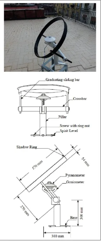
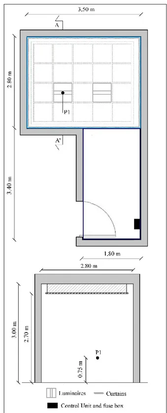
IV.1. Room description ... 31
IV.2. Setting up of the measurement system ... 31
IV.3. Luminaires characteristics ... 35
IV.4. Lighting system design ... 37
IV.5. Definition of the calculation parameters to set in DET ... 37
V. Case study results ... 41
V.1. Daylight measurements results ... 41
V.2. DLCSs performances results ... 56
VI. Discussion ... 73
VII. Merits, limitations and future steps of the research ... 75
Conclusions ... 77
Appendix ... 81
A.1. Open-loop switching ... 81
A.2. Closed-loop switching ... 84
A.3. Open-loop stepped ... 84
A.4. Closed-loop stepped ... 86
A.5. Open-loop dimming ... 88
A.6. Closed-loop integral reset ... 89
Introduction
In the last few decades daylighting has earned again the key role it deserves as a fundamental part of lighting design. As it has been underlined in the recent IES RP-5-13 report [1], the role of electric light is basically to integrate daylight when it is absent or inadequate to guarantee alone visual tasks performing. This means that, despite electric light gives us the possibility to create whatever lighting condition, daylight must be considered the fundamental light source in indoor environments, especially in those spaces where people perform their every-day life activities and remain for most of the day (workplaces, offices, schools, hospitals, etc).
The attention about daylighting themes is driven by two issues, that by now have become crucial in modern building design culture: on one hand the care about themes concerning energy savings and natural energy sources exploitation; on the other hand, the will to improve more and more users’ comfort conditions in indoor spaces. About these topics, modern researches have repeatedly highlighted the strict connection between the use of daylight and the reduction of energy consumptions [2-6]; however, daylighting benefits are even more important, if we consider the direct incidence on people wellness. Researches demonstrated that daylight not only influences visual comfort, but it has non-visual effects as well [7]. It is one of the main regulators of the circadian rhythms [8], influences people’s mood and has a fundamental role in defining people’s alertness state, work performances and productivity [9].
From this perspective, daylighting design becomes again a primary step, not only of lighting design, but also of building design in general, since aspects like building shape or façades configurations obviously affect daylight entering in indoor spaces.
This makes crucial studies about technologies allowing indoor daylighting to be improved, controlling at the same time the correlated risks (glare, overheating): innovative shading systems, smart façades, daylight transportation devices [10].
Moreover, the use of automated systems, able to manage the integration of daylight and electric
light, becomes fundamental: these systems reduce electric light usage, increasing energy savings and, at the same time, they allow light to be tailored to people’s needs [11]. These devices are commonly known as daylight-linked control systems (DLCSs). They are based on the use of photosensors installed inside or outside the building, that detect incident daylight, send a signal to a controller. The controller, in turn, regulates luminaires light output. The regulation actions goal is to integrate daylight and electric light, in order to maintain average work-plane illuminance levels around the limits indicated by regulations.
The development of such systems has certainly been boosted by the spread of new LED light sources and of related electronic management systems. According to [12], sophisticated lighting controls use is supposed to increase so that, considering all buildings typologies together, the related revenue from their installation is expected to grow at 14.3% compound annual growth rate between 2017 and 2026.
However, the functioning mechanism of these systems is not yet completely clear. Factors affecting their performances are too many (photosensors characteristics and location, adopted control strategy, lighting systems components features [13]) and not easy to control during both the design phase and the commissioning one. Thus, once they have been installed, DLCSs operate differently from the expectations: illuminance levels are too low or too high compared to the required ones [14], luminaires are turned on and off not properly [15], electric light fluctuations are too frequent and annoy users [16].
The predictable consequence is that users, verifying the improper functioning of the automated controls, disable them and all the presumed benefits are unavoidably lost. It must not be forgotten that the effectiveness of DLCSs strictly depend on the users’ grade of acceptance. Previous works, indeed, demonstrated how much is important for people to exercise a direct control in the management of the environment they live in [17]. Moreover, studies based on surveys demonstrated that often people prefer manual than automated control [18], and that, when automated systems are installed, they are more satisfied having the possibility to partially override the
automated control [15, 19]. Moreover, the grade of acceptance of automated controls strictly depends on spaces function and it is major when spaces are perceived not belonging to anyone (e.g. atria, corridors or circulating areas) [20, 21].
Thus, it is fundamental to design automated controls guarantying proper lighting conditions, in order to avoid users disable them.
Given these premises, what are the main causes generating difficulties in DLCSs project? How can they be solved?
Currently the pressing problems are the following:
• As it was previously reported, factors affecting DLCSs performances are many, but it is not completely clear what is the specific incidence of each one of them on DLCS global functioning [22];
• It is crucial for designers to be able to simulate DLCSs operating conditions during the different design stages, in order to evaluate benefits connected to their installation. However, despite the development of dynamic daylight simulation methods and the spread of sophisticated calculation software, DLCSs simulation is neither immediate nor reliable. Indeed available calculation tools are not able to account for all the affecting factors [23] and consequently predicted energy savings turned out to be different from those observed in the field [24];
• Even though performing a reliable simulation was possible, the evaluation of the global performance of these systems is not easy. Generally, DLCSs are assessed exclusively depending on energy savings they allow achieving. This is a too simplistic and not reliable assessment method: these systems sometimes, even providing significant savings, operate so that lighting requirements are not fulfilled. So, how is it possible to evaluate this aspect? Currently, common and shared parameters useful to evaluate DLCSs performances do not exist. So, not only it is problematic to evaluate the convenience in installing such systems, but it is also difficult to assess their performance during the operating life [25].
All these problems determine a poor DLCSs design culture: automated lighting controls based
on daylight exploitation are often sold as a ready-made product, sometimes integrated in a wider control network (Building Management Systems -BMS) and designers install them without being really aware of all connected design issues.
Given these premises, the goal of the thesis is to try to suggest a design methodology for DLCSs, accounting for the above-mentioned issues. To do that the work is divided in the following sections:
• Analysis of the state of the art, necessary to collect available information about factors affecting DLCSs performances;
• Definition of new performance metrics useful to evaluate DLCSs capability in integrating daylight;
• Analysis of the current available software to simulate DLCSs and of the related limits; • Development of a calculation tool trying to
overcome these limits, allowing a more reliable simulation of DLCSs;
• Implementation of the proposed performance parameters calculation module in the above-mentioned simulation tool;
• Use of the tool and of the proposed parameters to verify the performance of different typologies of DLCSs in a real space.
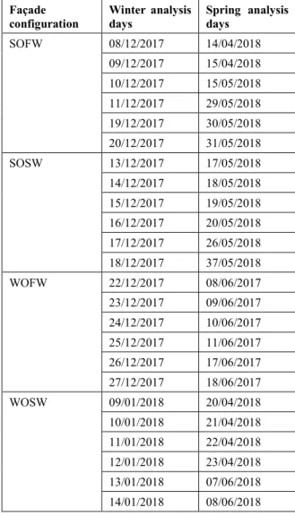
It must be underlined that the developed tool evaluates DLCSs performances starting from indoor daylight availability data. These data can be inferred from both simulations and field measurements. For the thesis application, measured data were used. For this purpose, a specifically developed monitoring system was set up. An office located in one of the buildings of the University of Naples “Federico II” was used as case study. Daylight irradiance and illuminance measurements were performed during winter and spring, in order to obtain real daylight data referred to work-plane illuminances and photosensors detections. These data were then uploaded in the calculation tool to evaluate the performance of different DLCSs typologies, to verify their seasonal functioning and compare them, to observe the factors affecting their performances and to identify the most suitable control strategies.
Analysis methodology presented in the thesis and part of the results, were published during the PhD course in [13, 22, 25-27].
I. Daylight-linked control systems (DLCSs): functioning and affecting factors
DLCSs are automated control systems, able to manage luminaires based on indoor daylight availability. One or more photosensors detect incident light and send a signal to a controller. The controller, according to the received information, switches on and off or continuously regulates luminaires emitted flux, in order to integrate available daylight by means of electric light and to guarantee lighting requirements at the work-plane. Despite the simplicity of the base concept DLCSs are based on, designing such systems is not an easy task, due to the big quantity of factors affecting their performances. Following paragraphs propose an analysis of these factors. According to [22], the order factors are presented recalls DLCSs design process, starting from daylight availability evaluation and going ahead with the control strategy definition and the lighting system components choice, finally concluding with the commissioning.I.1. Daylight availability
Considering that the goal of DLCSs is to reduce the use of electric light maximizing that of the natural one, it is clear that their performances depend first and foremost on the daylight availability characterizing the spaces they are installed in. Previous studies focused on this issue and tried to underline how achievable energy savings can vary depending on all those parameters that influence daylight availability: building orientation and location, weather conditions, shading devices typologies and so on.
For example, Roisin et al. [28] calculated energy savings achievable in an office by using the same DLCS, but varying the orientation and the location of the room. They considered three different cities (Brussels - latitude 50° 51' N, longitude 4° 20' E; Athens - latitude 37° 58' N, longitude 23° 42' E and Stockholm - latitude 59° 19' N, longitude 18° 3' E) and the four main orientations. They found that savings ranged from 46%, considering the worst case (Stockholm – north orientation), to 61%, considering the best one (Athens – south orientation.
The effect both of the seasonal changes and of weather conditions was analyzed by Onaygil and Güler [29]. They observed the case of a north-east oriented office in Istanbul (latitude 41° 0' N, longitude 28° 56' E) equipped with a lighting system managed by a dimming DLCS. The researchers found that energy savings were 27% higher in June and July, if compared with those achieved in December. Moreover, they calculated that savings were equal to 35% in presence of clear skies and to 16% in presence of overcast ones.
Not only the global amount of daylight entering a space affects the way a DLCS functions, but also its spatial distribution. This topic was faced by Galasiu et al. [30], who examined the case of an open-space office, equipped with workstations arranged in different rows. Each workstation was lit by a luminaire equipped with an integrated photosensor. In this way it was possible to properly regulate luminaires flux emission depending on the daylight available at the single desk. Researches underlined how the savings can vary in the same room according to the workstation distance from the window. Specifically, they obtained the following results: depending on the considered season, the savings ranged from 17% to 24% in the perimeter workstations, from 9% to 20% in the second row and from 9% to 16% in the most interior one.
Other studies focused on the interactions between lighting control systems and shading devices. Even if this topic deserves a specific treatise, some studies will be cited to give a general idea of the problem.
Lee et al. [31] observed how the variation of venetian blinds tilt angle can determine a change in the ratio of the work-plane illuminance to the photosensor signal, finally modifying the way DLCSs operate. Galasiu et al [32] calculated energy savings achievable by means of simple switching and dimming systems in a space were different typologies of manual and photocontrolled venetian blinds were installed. Researchers found that, in presence of clear sky, the use of shading devices could reduce achievable energy savings from 5% to 45% in dimming system case and from 5% to 80% in switching system one.
The research of a balance between the maximization of energy savings due to daylight use and the necessity to avoid glare and overheating is an ambitious challenge that some researchers have accepted [33-35]. For example, Shen and Tzempelikos [34] developed an advanced integrated thermal and simulation model to evaluate daylighting and energy performances in private offices with automated interior roller shades. The tool was meant to be used during the design process to identify the most suitable technical choices, accounting for both thermal and lighting issues. Moreover, Shen et al. [35] studied the way to integrate the control both of shading devices and lighting controls with that of HVAC systems as well.
I.2. Control strategy definition
The definition of the control strategy consists in establishing the way the control system operates. Basically, DLCSs can be divided in open-loop and closed-loop ones. The former ones are managed by photosensors detecting exclusively daylight. For this reason, they are installed outside the building (on the roof or on the façade) or inside it, but in this latter case they are located and oriented such to detect exclusively daylight, for example, they look toward a window. In closed-loop systems, photosensors are located in the same room where the control is performed, and they detect both daylight and electric light.
DLCSs can be classified also according to the actions actuated by the controller. In this case we have switching systems, stepped systems and dimming ones. In the first case luminaires are simply switched on and off according to the photosensor detections. Stepped systems are similar to the switching ones, but luminaires can be turned on and off reaching different light output levels (generally two or three), for example 50% and 100%. Finally, dimming systems continuously regulate luminaires flux emission, proportionally to the variations of light levels detected by the photosensor. Depending on the combination of the photosensor typology and of the action actuated by the controller, the corresponding control algorithm can be identified. Basic control algorithms (open-loop and closed-loop switching, open-closed-loop and closed-closed-loop
stepped and open-loop and closed-loop dimming) are in-depth described in the Appendix.
Control strategy should be properly chosen depending on the specific case. Atif and Galasiu [36] calculated energy savings achieved in two buildings atria: the former equipped with a dimming system and located in Québec City (latitude 46° 48' N, longitude -71° 12' W); the latter equipped with an on-off switching system and situated in Ottawa (latitude 45° 24' N, longitude 75° 41' W). In the former case savings were equal to 46%, in the latter equal to 17%.
Chiogna et al. [37] monitored the functioning of DLCSs installed in two groups of south-exposed lecture rooms, located in Trento (latitude 46° 04' N, longitude 11° 08' E). They found that the use of an on-off switching system, coupled to an occupancy-based one, provides savings equal to about 40%. Integrating occupancy-based control with a dimming DLCS, savings increased till 65%.
However, Li et al. [38] reported that, differently from what would seem obvious, dimming systems are not always more advantageous than switching ones. According to the researchers, indeed, the benefits deriving from a strategy or another depend both on the daylight availability and on the required task illuminance. Switching systems could turn out to be more advantageous if a low task illuminance value is required and daylight levels are generally high [39].
Rubinstein et al. [38] studied experimental results obtained by means of scale models located on the roof of the third floor of Building 90 at Lawrence Berkeley Laboratory (latitude 37° 52′ N, longitude 122° 16′ W). They compared energy savings achievable by adopting different control strategies and they found that the best results were provided by closed-loop dimming systems.
There are two different typologies of closed-loop dimming systems: integral reset and proportional dimming. Some studies compare these two strategies. Mistrick et al. [40] found that integral reset was not suitable for sidelit spaces. This is due to the fact that the system is calibrated exclusively in presence of electric light, neglecting the daylight contribution. On the contrary proportional dimming calibration procedure accounts for the fact that daylight and
electric light determine different ratios of work-plane illuminance to photosensor signal.
Doulos et al. [41] focused on the same issue. They observed that, in a south-oriented office located in Athens (latitude 37° 58' N, longitude 23° 42' E), proportional dimming systems provided savings ranging from 66.91% to 72.82%, whereas integral reset allowed obtaining higher savings, ranging from 70.35% to 76.09%. However, researchers observed that often integral reset operated so to determine illuminance levels at the work-plane lower than those prescribed by regulations, meaning that part of the energy savings were due to an improper system functioning.
Ihm et al. [3] studied the performances of different DLCSs installed in offices located in Chicago (latitude 41° 51' N, longitude -87° 39' W). They found that dimming systems generally provide higher savings compared with stepped ones. However, this difference decreases on windows glazing area increasing.
I.3. Photosensors choice
Characteristics of photosensors affect the functioning of DLCSs. So, it is fundamental to properly choose its characteristics: “spatial
response (the sensitivity in detecting the incident radiation coming from different directions), spectral response (the sensitivity in sensing the incident radiation depending on different wavelengths) and range of response (a limited range of output signal values in which light measurement is accurate”[22].
All these features, indeed, contribute to define the ratio of the daylight work-plane illuminance, 𝐸̅𝑑𝑙, to the daylight photosensor signal, 𝑆𝑑𝑙. This ratio is at the basis of DLCSs calibration procedures and the more it maintains itself steady over time, the more the performances of the system are good.
Doulos et al. [42] studied the relative spectral responses of five typologies of photosensors and verified that they were broader than the V(λ) function. Moreover, they observed that the related sensitivity peak corresponded to about 540.9 nm to 600.7 nm. The fact that photosensors spectral response does not match the V(λ) reduces the reliability of detections and obviously has an
impact on the global functioning of the DLCSs. In another study [43] the researchers quantified this impact in terms of energy savings, analyzing the performance of different photosensors in a room where window glazing was varied in order to modify the spectrum of entering daylight. They observed differences from 0.37% to 5.44% depending on the analyzed case.
The effect of spatial response was studied by Rubinstein et al. [44], who suggested preferring photosensors characterized by high fields of view and to shield them from the direct light of the window. On the contrary Ranasinghe and Mistrick [45] found that the narrower the photosensor field of view is, the better the system functions.
To solve problems connected to the reliability of photosensor detections, manufacturers and researchers proposed different solutions. One of this is the use of luminaires with integrated photosensors. In this way lighting can be managed according to different criteria in different zones of the same room and the lighting conditions sensed by photosensors should be more representative. Management of these systems is not so easy, and several studies have been published in this regard [46-50]. They focused on defining photosensors networks, to integrate DLCS strategy with occupancy-based ones associating occupancy sensors with light ones. Moreover, they propose the idea that in open-space offices, each user occupying a different workstation can auto-calibrate the control of his own lighting. Obviously, this determines other problems. People have different preferences about luminous environment considering both light intensity and color [51]. This could create in open-space offices unpleasant and not uniform global lighting conditions.
Moreover, research suggested installing devices different from the standard photosensors. Some researches proposed to use CCD (Charge-Coupled Device) cameras or CMOS (complementary metal-oxide semiconductor) image sensors [52-54]. These devices are able to measure luminance distribution of the workstations, controlling at the same time lighting and occupancy conditions. However, these systems present limits as well. On one hand it is not easy to identify precise algorithm starting from luminance maps, especially considering that accidental factors, such as the furniture relocation,
could invalidate the calculation model [52]. Moreover, the now available devices are characterized by costs too high to be used in common applications [54].
I.4.
Lighting
system
component
characteristics
When a DLCSs is installed, all the components of the lighting system must be compatible. Different studies underlined how lamps and luminaires characteristics affect DLCSs performances, but, at the same time, the control itself can influences them. For example [55] underlined the necessity to set special time delay, when high intensity discharge lamps are used, in order to account for the restrike time. Moreover, the minimum light output, which the luminaires can be dimmed at, is not the same for all lamp technologies [3]. It must also be considered that continuous on-off switching could reduce lamps life. Tetri [56] underlined that considering fluorescent lamps, switching systems affect lamps life more than the dimming ones and that the use of electronic dimming ballasts helps lamps to maintain their nominal life.
A lighting system fundamental component is the ballast, i.e. the device that controls luminaires light output according to the photosensor detections. Each ballast is characterized by a specific dimming response function, i.e. a curve describing the relationship between photosensor signal and the light output. Before LED luminaires spread, dimming ballasts managing fluorescent lamps were based on an analog 0-10 V control protocol [11]. Some studies, underlined that, since there was not a lighting specific standard to define the correspondence between the received analog signal and the light output, starting from the same signal, using different ballasts, the controller could generate different light outputs. For example, Doulos et al. [41], comparing the way to operate of different ballasts, underlined that the same 5 V signal produced a light output varying from 8.90% to 54.89%, in turn corresponding to a relative absorbed power varying from 20.20% to 60.09%. This obviously influenced energy savings, that varied from 66.91% to 72.82% with a proportional system and from 70.35% to 76.09%, considering reset control. A similar study was performed by Roisin et al. [28], who compared the
characteristics of analog systems and digital ones and underlined that digital controllers and related sensors were characterized by energy consumptions higher than analog one. For this reason, the use of digital systems turned out to be more advantageous if a single controller and a single photosensor were responsible to manage different luminaires together, whereas in stand-alone applications the analog ones was profitable.
The spread of LED sources, managed by means of digital controls, has boosted the interest towards the dynamic lighting [51]. For these sources the regulation of emitted flux is more stable than for the traditional ones, and as it was demonstrated by previous researches [46, 47] the relationship between luminaires power consumption and dimming level can be assumed to be linear.
However, in some cases LED dimming can determine undesired perceivable chromatic shifts. For these reasons some studies have focused on the research of methods to control changes in spectral power distribution due to light output variations [57, 58]. Moreover, some LED sources, when dimmed, determine visible or invisible flicker, that could be dangerous for people health [59]. This issue was investigated in [60]. Light frequencies responsible to induce biological human response were found and methods to mitigate the biological effects were discussed.
When lighting controls are designed, another important issue to consider is the impact of stand-by energy use. Gentile and Dubois [61] reported that it represents about the 30% of the total lighting energy use, reaching in extreme cases 55% value. They argued that when standby energy use cannot be minimized, in individual offices or similar applications the use of very efficient light sources can be sufficient and reduce the necessity to design complex controls.
Another crucial aspect is the control zones setting. A control zone is an area lit by luminaires all managed in the same way. Li et al [38] deepened this issue, experimenting different strategy of grouping luminaires. The experiment was performed in a classroom equipped with three rows of fluorescent luminaires arranged parallel to the window. The researchers calculated energy savings by varying the way the control was operated and found that energy savings varied from 23.4% to 70.4%. In the most
disadvantageous case only the row nearest to the window was automatically switched on and off, whereas the others were manually controlled. On the contrary, in the most advantageous case, the row nearest to the window were independently and automatically switch on and off, whereas the row farthest from the window was continuously dimmed.
Galasiu et al. [30] studied the possibility to differently control lamps belonging to the same luminaire. They analyzed the case of luminaires installed in an open space office, equipped with three 32 W fluorescent lamps, one upward directed and two downward directed. They observed that, if the uplight was fixed and the downlight was dimmed depending on daylight availability, daily average savings were equal to 32% in spring and summer and equal to 16% in winter. If all the lamps were dimmed, savings became 47% in spring and summer and 24% during winter.
Caicedo et al. [48] studied LED luminaires generating two different and independent optical beams: one wider and the other narrower. The former was used to provide ambient lighting, the latter to obtain task lighting. Luminaires were equipped with both photosensors and occupancy sensors. The narrowest light beam was turned on and off according to people presence absence in the controlled area and the widest was regulated according to the daylight availability.
I.5. Commissioning
Commissioning consists in the setting of the control system and in the check of its operative conditions during the system life cycle. The correct installation and commissioning is fundamental to guarantee the good performances of control systems [62].
The setting of the control is defined calibration. The calibration procedure is different from each control strategy (see the Appendix). However, generally, it consists in defining the ratio of the daylight work-plane illuminance to the daylight photosensor signal (𝐸̅𝑑𝑙/𝑆𝑑𝑙), in order to establish luminaires light output necessary to integrate daylight. To do that the critical task location (i.e. the point receiving the smallest quantity of daylight) must be identified; the related
work-plane illuminance must be measured together with the photosensor signal; the necessary light output must be set. From the calibration on, the system will work considering that the ratio of the work-plane illuminance to the photosensor signal, despite daylight availability variations, remains constant and equal to that measured at the calibration phase.
However, researches [40, 63] underlined that this is not true and that this ratio continuously changes depending on indoor daylight distribution.
Choi et al. [64] focused on this issue observing the functioning of different photosensors located in an office in Seoul, Korea (latitude 37° 33' N, longitude 126° 58' E). They underlined that the ratio of work-plane illuminance to the photosensor signal strictly depends on sensor location, its aiming angle and sky conditions.
Chiogna et al. [65] deepened this aspect in an office located in Sesto al Reghena, Pordenone, Italy (latitude 45° 57' N, longitude 12° 39' E). They observed that, when outdoor daylight conditions are similar, similar 𝐸̅𝑑𝑙/𝑆𝑑𝑙 ratio were observed. Consequently, they proposed to implement the control algorithm by means of seasonal correction functions, accounting for the seasonal 𝐸̅𝑑𝑙/𝑆𝑑𝑙 variations.
Recently Beccali et al. [66] proposed a method based on artificial neural networks to identify the best photosensor location during design and commissioning phase.
During calibration other parameters such as time delays, minimum and maximum light output are set as well.
Littlefair [16] focused on continuous electric light oscillations in switching systems disturbing users and due to frequent outdoor daylight fluctuations. To reduce them he suggested to introduce time delays equal to 30-45 minutes.
A similar study was performed by Li et al. [67] who analyzed different switching techniques: “daylight-linked time delay (lights can be switched
off only if daylight illuminances exceed a specific target value), switching-linked time delay (lights cannot be switched off if a specific time is not elapsed from the last switching-on), solar reset switching (a reset time is set and only when reset time occurs, daylight levels are monitored: if they
are higher than target value, lights are switched off)”[22]. They found that the daylight-linked
time delay was the strategy providing the most significant reduction of switching actions.
Bellia et al. [26] compared the effectiveness of different switching techniques in an office located in Naples (Latitude 40° 51' 22 N, Longitude 14° 14' 47 E). They found that the better performance was guaranteed by means of switching-linked time delay and that solar reset systems turned out to be
the worst. Researchers also suggested that “the
problem of the brusque oscillations cannot be avoided unless it is accepted to introduce a time delay for switching on actions as well” [26]. They
underlined that previous researches [19] demonstrated that people sometimes choose illuminances lower than those prescribed by regulations. Consequently, it is possible that users would prefer occasionally low light levels compared to continuous and sudden switching on actions.
II. New parameters to evaluate the capability of DLCSs in integrating daylight
Previous paragraphs demonstrated that the number of factors affecting DLCSs functioning is huge. Consequently, it is fundamental to be able not only to evaluate performance of automated control systems, but also to understand how the different factors influence their operating conditions. As it was mentioned in the Introduction, nowadays DLCSs are exclusively evaluated considering energy savings they produce. The following paragraphs are explaining why this approach is not sufficient and are introducing new parameters useful to evaluate the capability of DLCSs in integrating daylight.II.1. Today available parameters and their
limits
The birth and the spread of dynamic daylight simulations have provided new possibilities in the daylighting research field. Obviously, this has had an impact on the evaluation of the benefits connected to the installation of DLCSs. Indeed, the possibility to accurately know daylight availability variations during time (accounting for weather conditions, daily and seasonal rhythms) should allow the electric light requirement of a specific space to be estimated. Then, starting from the requirement, it should be easy to evaluate what is the electric lighting system most suitable to integrate daylight and fulfill the calculated requirement. Actually, problems connected to lighting systems dynamic modelling are complex and the related evaluations about their performances and the connected benefits are not immediate.
After the introduction of dynamic daylight simulations, the main problem was to find indices able to synthetically describe daylight availability in indoor environments. Software for dynamic calculations upload weather data file and, based on the related information, define sky luminance distribution for each record of the weather data file (generally corresponding to an hour of the year). Finally, accounting for the optical characteristics of architectural surfaces, they evaluate interactions between daylight and space and calculate for each hour of the year illuminance values at specific points belonging to calculation grids set by users [68]. In some cases, thanks to proper interpolation models, results referred to fractions of hour, e.g. half an hour, 5 minutes or 1
minute [69] can be obtained. This provides an enormous amount of data not easy to be managed. Therefore, statistic indices have been introduced to summarize and comment dynamic daylight simulation results such as Daylight Autonomy (DA) [70], Continous Dayligth Autonomy (DAcon) [70], Useful Daylight Illuminance (UDI) [71, 72]. These indices are partially useful also to evaluate DLCSs.
DA represents the time percentage of occupied hours of a year during which daylight illuminance at the work-plane is equal or higher than the task illuminance prescribed by regulations [73]. This means that ideally, during these hours, electric lights could be completely off.
DAcon accounts for the fact that daylight contribution should be considered even if the corresponding illuminance is lower than the task illuminance prescribed by regulations. So, the DAcon is the percentage ratio of the daylight illuminance to the task illuminance. If for example for the 30% of the year, the work-plane is characterized by DAcon value of 80%, it means that, ideally, using a dimming control system, luminaires light output could be equal to 20% for the 30% of the year.
UDI gives us similar information. It is the percentage of the occupied hours of a year during which daylight illuminances are comprised in the range 100 lx – 2000 lx. Based on surveys performed in offices, this range is considered useful by people, since it corresponds to light levels neither too dark nor too bright. The useful range can be divided in two further steps UDIsupplementary (from 100 lx to the task illuminance) and UDIautonomous (from the task illuminance to 2000 lx. It must be underlined that
the lower limit of this range is general considered equal to 100 lx (300 lx in [74]), whereas authors do not agree about the setting of the upper limit: it is equal to 2000 lx in [72], 2500 lx in [75], 3000 lx in [76], 8000 lx in [74]. Based on UDI definition, to have an idea about the operation range of a daylight-linked control system, it is necessary to evaluate when daylight illuminance is lower than 100 lx or it falls in UDIsupplementary.
These parameters allow evaluating the daylighting potential of a space and are useful to have a preliminary idea about the convenience to install or not a DLCS. However, they are based exclusively on the space characteristics without considering the features of a real lighting system. For this reason, simulation software have been implemented by means of tools useful to simulate the dynamic functioning of lighting systems, managed by different typologies of automated controls [77, 78] (a focus on available software to simulate control systems is reported in paragraph III.1). This has allowed obtaining annual scheduling related to lighting system absorbed power and, consequently, to evaluate connected energy consumptions. This has provided the possibility to evaluate the performances of control systems according to energy savings provide. Generally, the savings are estimated considering a reference lighting system switched on at 100% for the entire year.
However, achieved energy savings are not a very reliable indicator of DLCSs performances. For example, if two systems characterized by the same technical features are installed in two spaces with different daylight availability, they would provide different savings. This doesn’t mean that the system characterized by lower savings works improperly, but only that the two spaces are characterized by a different potential in terms of daylighting. On the other hand, high energy savings could be the consequences of an improper functioning of the system. For example, a DLCS, that is wrongly calibrated, could determine illuminance levels at the work-plane often lower than those prescribed by regulations. This would reduce energy consumptions to the detriment of lighting quality.
Thus, specific parameters are necessary to describe the performance of DLCSs. Considering
that their goal is to integrate daylight, DLCSs should be evaluated according to their capability in maintaining proper indoor light levels, complementing daylight and not on the basis of the achieved savings.
In this respect, it is interesting the work by Doulos et al. [79]. They proposed a multi-criteria analysis methodology useful to identify the optimum position and the proper field of view of the photosensors during the design process. To do that, they suggested to consider two additional parameters beyond the achieved energy savings: the correlation between work-plane illuminance and photosensor signal and the lighting adequacy. The former parameter is useful to control the effect of photosensor characteristics on systems performances. On the other hand, the lighting adequacy is defined as: “the percentage for occupied time with total illuminance exceeding design illuminance” [79], where total illuminance is the sum of work-plane daylight and electric light illuminances. This parameter introduces a fundamental concept: an ideal DLCS should be able to perfectly adapt electric light emission to daylight variations, so that the sum of the work-plane daylight illuminance (𝐸̅𝑑𝑙(𝑡)) and work-plane electric light illuminance (𝐸̅𝑒𝑙(𝑡)) should be always equal to the average maintained illuminance prescribed by regulations (𝐸̅𝑡𝑎𝑠𝑘). Obviously, this is impossible owning to the real technical characteristics of DLCSs. So, the total illuminance 𝐸̅𝑡𝑜𝑡(𝑡) determined by the control system can be higher or lower than 𝐸̅𝑡𝑎𝑠𝑘, depending on the way the system reacts to photosensor detections. The specific goal of the lighting adequacy is to evaluate the time percentage of the observation period during which the system is able to guarantee prescriptions, i.e. it is verified that 𝐸̅𝑡𝑜𝑡(𝑡) is equal or higher than 𝐸̅𝑡𝑎𝑠𝑘. The complement to 1 of the light adequacy informs about an improper control system functioning, corresponding to 𝐸̅𝑡𝑜𝑡(𝑡) values lower than 𝐸̅𝑡𝑎𝑠𝑘.
A similar analysis approach was proposed by Bonomolo et al. [14], who introduced two indexes: OAR (Over illuminance Avoidance Ratio) and UAR (Under-illuminance Avoidance Ratio). These indexes describe the capability of
the system in reducing over-illuminance and under-illuminance conditions, i.e. in avoiding that 𝐸̅𝑡𝑜𝑡(𝑡) is higher or lower than 𝐸̅𝑡𝑎𝑠𝑘 respectively. The more the indices are close to 1, the better the system operates.
Based on the proposals of [14, 79], new parameters have been introduced [25, 27] during the PhD. course. They are: Daylight Integration Adequacy (𝐷𝐼𝐴), Percentage Light Deficit (𝐿𝐷%), Percentage Intrinsic Light Excess (𝐼𝐿𝐸%) and Percentage Light Waste (𝐿𝑊%).
The parameters are based on issues proposed by [14, 79], but introduce a new concept: the intrinsic light excess. They will be fully described in the following paragraph.
II.2. The rationale for the definition of the
new parameters
Standards [73] prescribe that electric lighting systems have to guarantee specific values of average maintained illuminances at the work-plane (𝐸̅𝑡𝑎𝑠𝑘), different depending on the performed visual task.
Given a period 𝑇 (for example the number of occupied hours of a space during a month, a season or a year) we can define the Light Requirement, 𝐿𝑅, of the work-plane during 𝑇, in terms of light exposure as:
𝐿𝑅 =𝐸̅𝑡𝑎𝑠𝑘∙ 𝑇 [lx∙h] (II.1)
When a room is daylit, daylight can satisfy part of 𝐿𝑅, since at each time 𝑡, the work-plane receives a certain amount of daylight, corresponding to an average daylight illuminance 𝐸𝑑𝑙,𝑡. Since, daylight availability varies with time, it is possible to define the function 𝐸𝑑𝑙(𝑡). The integral of this function over 𝑇 is defined Daylight Exposure, 𝐷𝐸.
𝐷𝐸 = ∫ 𝐸𝑑𝑙(𝑡)
𝑇
𝑑𝑡 [lx∙h] (II.2)
1 All the figures of this section are referred to data measured
on the 22nd of December 2017, in the test-room used as case
The Light Requirement fulfilled by daylight, 𝐿𝑅𝑑𝑙 can be evaluated as:
𝐿𝑅𝑑𝑙= ∫ 𝐸̅∗𝑑𝑙(𝑡)𝑑𝑡 𝑇 [lx∙h] (II.3) Where: 𝐸̅∗ 𝑑𝑙(𝑡) = { 𝐸𝑡𝑎𝑠𝑘 𝑖𝑓 𝐸̅𝑑𝑙(𝑡) ≥ 𝐸𝑡𝑎𝑠𝑘 𝐸̅𝑑𝑙,𝑡 𝑖𝑓 𝐸̅𝑑𝑙(𝑡) < 𝐸𝑡𝑎𝑠𝑘 [lx] (II.4)
The ratio of 𝐿𝑅𝑑𝑙 to 𝐿𝑅 is a good indicator of the daylight availability characterizing the analysed space.
A DLCS is supposed to operate so that when 𝐸𝑑𝑙(𝑡) assumes values higher than 𝐸̅𝑡𝑎𝑠𝑘 luminaires are off, whereas, when it assumes values lower than 𝐸̅𝑡𝑎𝑠𝑘, luminaires flux is properly regulated to integrate daylight.
Figure II. 1: Daylight illuminance and ideal electric light illuminance at the work-plane
An ideal and perfectly functioning automated control, based on dimming strategy, at each time 𝑡, should determine at the work-plane an electric light illuminance value (let us call it ideal electric light illuminance, 𝐸𝑒𝑙,𝑖𝑑,𝑡 -see Figure II.11-) so that it is possible to define the function:
𝐸̅𝑒𝑙,𝑖𝑑(𝑡) = 𝐸̅𝑡𝑎𝑠𝑘-𝐸̅∗𝑑𝑙(𝑡) [lx] (II.5)
and a task illuminance equal to 750 lx was considered. All the details about the case study are reported in the IV Section.
Obviously, given its technical characteristics, a real control system determines electric light illuminances over time, 𝐸𝑒𝑙(𝑡), different from the ideal ones (see Figure II.2). When 𝐸𝑒𝑙(𝑡) is higher than 𝐸̅𝑒𝑙,𝑖𝑑(𝑡), a light excess occurs. Conversely, when 𝐸𝑒𝑙(𝑡) is lower than 𝐸𝑒𝑙,𝑖𝑑(𝑡), prescribed light requirements are not fulfilled and a light deficit arises.
Figure II. 2: Comparison between the ideal electric light illuminance and that provided by a real system
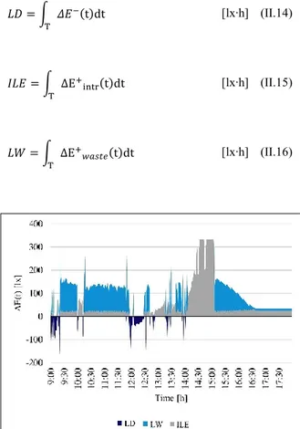
Figure II. 3: ΔE(t) function
The function 𝛥𝐸(𝑡), representing at each time 𝑡 the difference between 𝐸𝑒𝑙(𝑡) and 𝐸𝑒𝑙,𝑖𝑑(𝑡), well describe the performance of a DLCS (see Figure II.3).
Shifts of 𝐸𝑒𝑙(𝑡) from 𝐸𝑒𝑙,𝑖𝑑(𝑡) can be determined by all the factors described in the Section II. We can divide all these factors in two categories, those that are communal for all design strategies (e.g. daylight availability or photosensors characteristics) and those strictly depending on the adopted control strategy (e.g. number of steps in stepped systems or minimum
light output in dimming systems). The two categories of factors determine different effects.
To better understand that, let us consider the case of an open-loop proportional dimming system. It operates so that luminaires light output is continuously regulated according to photosensor detections, varying from a maximum value (𝛿𝑚𝑎𝑥) to a minimum one (𝛿𝑚𝑖𝑛), without ever being switched completely off (see Figure II.4).
Figure II. 4: Open-loop dimming control algorithm
This system can be calibrated by defining two set points: the former one is set during night, when daylight is absent and luminaires must be turned on at the maximum light output (𝛿𝑚𝑎𝑥); the latter is set during day, choosing the daylight photosensor signal, 𝑆𝑑𝑙,𝑡𝑐, corresponding to a work-plane daylight condition such that, to integrate 𝐸𝑑𝑙,𝑡𝑐 (daylight illuminance at the calibration) the required light output (𝛿𝑡𝑐) is higher than the minimum one (𝛿𝑚𝑖𝑛).
As it was reported in previous paragraphs, the choice of the 𝑆𝑑𝑙,𝑡𝑐 is crucial in determining system performance.
Figure II. 5: Relationship between photosensor signal and daylight work-plane illuminance
This is clear looking at Figure II.5. Let us assume that the above mentioned open-loop system is calibrated based on the couple illuminance-signal identified by the Point 1. When the condition represented by the Point 2 happens, a light excess occurs. Indeed, the photosensor signal in 2 is lower than that characterizing 1, so the system sets a light output higher than 𝛿𝑡𝑐. However, the daylight illuminance at the work-plane corresponding to the point 2 is higher than that registered at the calibration. The opposite happens when the daylight condition represented by the point 3 occurs: in this case a light deficit is produced. Problems connected to the variation of 𝐸𝑑𝑙(𝑡)/𝑆𝑑𝑙(𝑡) over time can determine both a deficit and an excess. Their effects can be diminished by calibrating the system as properly as possible and adjusting set-points during system life-cycle.
On the other hand, the factors depending on the control strategy always generated an excess. Effects of these factors cannot be avoided unless the strategy itself is changed. Considering the case of the open-loop dimming system, it remains always on at a 𝛿𝑚𝑖𝑛 value, even when daylight is sufficient alone to fulfil light requirements. Obviously, this generates light excesses. For switching systems excesses are even higher, considering that in this case luminaire luminous flux cannot be regulated, but lights are switched on every time the photosensor signal falls down a limit value.
It must be noticed that another cause of light excess is the fact that lighting systems are designed based on maintenance factors, used to account for luminous flux decay over time. So, during the first phases of the systems life cycle, when luminaires are on at 100% the produced illuminance at the work-plane is necessary higher than the task illuminance.
To distinguish light excess due to adopted control strategy from that due to the oscillations of 𝐸𝑑𝑙(𝑡)/𝑆𝑑𝑙(𝑡) (in turn depending on photosensor characteristics, location, daylight availability and so on), they will be called intrinsic light excess and light waste respectively. The intrinsic light excess also includes the excess due to the use of maintenance factors.
From the 𝛥𝐸(𝑡) function two different functions: 𝛥𝐸−(𝑡) and 𝛥𝐸+(𝑡), can be inferred:
ΔE−(t) = {0 if ΔE(t) > 0
−ΔE(t) if ΔE(t) ≤ 0 [lx] (II.6)
ΔE+(t) = {0 if ΔE(t) < 0
ΔE(t) if ΔE(t) ≥ 0 [lx] (II.7)
𝛥𝐸+(𝑡) in turn, can be seen as the sum of two different functions: 𝛥𝐸𝑖𝑛𝑡𝑟+ (𝑡), describing the excess due to the control strategy, and 𝛥𝐸𝑤𝑎𝑠𝑡𝑒+ (𝑡) describing the excess due to 𝐸𝑑𝑙(𝑡)/𝑆𝑑𝑙(𝑡) variations.
At this point it is necessary a procedure to calculate 𝛥𝐸𝑖𝑛𝑡𝑟+ (𝑡) and 𝛥𝐸
𝑤𝑎𝑠𝑡𝑒+ (𝑡). To evaluate 𝛥𝐸𝑖𝑛𝑡𝑟+ (𝑡) we have to neglect excesses due to 𝐸𝑑𝑙(𝑡)/𝑆𝑑𝑙(𝑡) variations. In order to do that, let us assume that the ratio 𝐸𝑑𝑙(𝑡)/𝑆𝑑𝑙(𝑡) is constant over time and that it is equal to the calibration ratio. EA,dl(t) Sdl(t) = EA,dl,tc Sdl,tc (II.8)
From the (II.8):
Sdl(t) = EA,dl(t) ∙
Sdl,tc
EA,dl,tc
(II.9)
At this point, it is possible to simulate the functioning of a reference system (see Figure II.6), i.e. a system with the same characteristics of the analysed one, but operating based on not-real photosensor detections, calculated according to the (II.9).
The reference system determines at the work-plane an electric light illuminance 𝐸̅𝑒𝑙,𝑟𝑒𝑓(𝑡) equal to:
𝐸̅𝑒𝑙,𝑟𝑒𝑓(𝑡) = δ𝑟𝑒𝑓(t) ∙ E̅el,100% [lx] (II.10)
δ𝑟𝑒𝑓(t) is calculated by means of the same equations used to evaluate 𝛿(𝑡) (they are all reported in the Appendix), but starting from photosensor detections obtained according to the (II.9). E̅el,100% is the electric light illuminance
determined by the system when luminaires are on at 100%.
Figure II. 6: Electric light illuminance provided by the reference system.
As it can be seen in Figure II.6., in dimming controls, the reference system functioning is really similar to the ideal one. The 𝐸̅𝑒𝑙,𝑟𝑒𝑓(𝑡) function is slightly higher that the 𝐸̅𝑒𝑙,𝑖𝑑(𝑡) one. This is due to the fact that the provided electric light illuminance in a real system is not perfectly equal to 𝐸̅𝑡𝑎𝑠𝑘, due to luminaires photometry characteristics. The part were the differences are significant corresponds to the moments of the day when the system could be turned off, but it remains on at minimum light output.
Starting from 𝐸̅𝑒𝑙,𝑟𝑒𝑓(𝑡) , it is possible to define the 𝛥𝐸+(𝑡) function related to the reference system (see Figure II.7):
∆Eref+ (t) = E̅el,ref(t) − E̅A,el,id(t) [lx] (II.11)
Figure II. 7: ΔE(t) function related to the reference system
Based on the (II.11) we can evaluate 𝛥𝐸𝑖𝑛𝑡𝑟+ (𝑡).
𝛥𝐸𝑖𝑛𝑡𝑟+ (𝑡) = {∆𝐸𝑟𝑒𝑓 + (𝑡) 𝑖𝑓 𝛥𝐸+(𝑡) ≥ ∆𝐸 𝑟𝑒𝑓+ (𝑡) 𝛥𝐸+(𝑡) 𝑖𝑓 𝛥𝐸+(𝑡) < ∆𝐸 𝑟𝑒𝑓+ (𝑡) [lx] (II.12)
When 𝛥𝐸+(𝑡) is higher than 𝛥𝐸
𝑖𝑛𝑡𝑟+ (𝑡), the residual excess cannot be due to the control strategy, but it is due to the oscillations of 𝐸𝑑𝑙(𝑡)/𝑆𝑑𝑙(𝑡). So:
𝛥𝐸𝑤𝑎𝑠𝑡𝑒+ (𝑡) = 𝛥𝐸+− ∆𝐸𝑖𝑛𝑡𝑟+ (𝑡) [lx] (II.13)
At this point, it is possible to correctly define the light deficit, 𝐿𝐷, the Intrinsic Light Excess, 𝐼𝐿𝐸, and the Light Waste, 𝐿𝑊 (see Figure II.8).
𝐿𝐷 = ∫ 𝛥𝐸−(t)dt T [lx∙h] (II.14) 𝐼𝐿𝐸 = ∫ ΔE+ intr(t)dt T [lx∙h] (II.15) 𝐿𝑊 = ∫ ΔE+ 𝑤𝑎𝑠𝑡𝑒(t)dt T [lx∙h] (II.16)
Figure II. 8: LD, LW and ILE
Given these premises it can be said that a DLC can function in four different operating conditions: ideal conditions (when the difference between 𝐸𝑒𝑙(𝑡) and 𝐸𝑒𝑙,𝑖𝑑(𝑡) is 0); light deficit, intrinsic light excess and light waste.
Once 𝐿𝐷, 𝐼𝐿𝐸 and 𝐿𝑊 concepts are described it is possible to finally introduce the new parameters.
Given a period 𝑇, 𝐷𝐼𝐴 (Daylight Integration Adequacy) is the percentage of time during which the control system operates in ideal or intrinsic light excess conditions. To better describe the system functioning 𝐷𝐼𝐴− and 𝐷𝐼𝐴+ can be evaluated. 𝐷𝐼𝐴− is the percentage of time during which the control system operates in light deficit conditions. 𝐷𝐼𝐴+ is the percentage of time during which the control system operates in light waste conditions.
Finally, 𝐿𝐷% (Percentage Light Deficit), 𝐼𝐿𝐸% (Percentage Intrinsic Light Excess) e 𝐿𝑊% (Percentage Light Waste) are respectively:
𝐿𝐷%= 𝐿𝐷 𝐿𝑅∙ 100 [%] (II.17) 𝐼𝐿𝐸%= 𝐼𝐿𝐸 𝐿𝑅 ∙ 100 [%] (II.18) 𝐿𝑊%= 𝐿𝑊 𝐿𝑅∙ 100 [%] (II.19)
The first three indices give us information about the occurrence during 𝑇 of the different operating conditions, the others about the quantity of light that is wasted or is lacking. To associate these different data is very important, as a simple example can demonstrate: if two systems have the same 𝐷𝐼𝐴− value, the number of hours during which a deficit occurs is equal. However, if 𝐿𝐷% values are different, as for the system characterized by the higher 𝐿𝐷% value, the differences between 𝐸𝑒𝑙(𝑡) and 𝐸𝑒𝑙,𝑖𝑑(𝑡) are on the average more significative compared with the other case. Obviously, a well-functioning system should not only reduce the time percentage during which the functioning is not ideal, but it should also reduce the more is possible the differences between 𝐸𝑒𝑙(𝑡) and 𝐸𝑒𝑙,𝑖𝑑(𝑡).
It is important to underline that the proposed parameters have a double value. Indeed, they are meant not only to be used as an evaluation tool during design stage, to identify the technical choices most suitable to the specific cases, but also as a commissioning control tool, to verify systems functioning during operating life.
III. DET: a new tool to evaluate DLCSs performances
The calculation of the parameters described in Paragraph II.1 is not immediate, since it is based on a dynamic approach. Moreover, it assumes that daylight illuminances at the work-plane over time -𝐸̅𝑑𝑙(𝑡)- are known, as well as the electric light illuminances determined by the control system -𝐸̅𝑒𝑙(𝑡)-. If the parameters are used to evaluate an already installed system, these data can be measured. On the contrary, if they are used to estimate systems performances during design process, dynamic daylight simulations are necessary.
Radiance-based software are universally recognised by researchers as the most reliable simulation tools to evaluate daylight availability with a dynamic approach [80]. Thus, they can be used to evaluate 𝐸̅𝑑𝑙(𝑡). On the contrary, the simulation of DLCSs is not yet an easy task [22], since, as it was already mentioned in the Introduction, it is pretty difficult to taking into account all the factors affecting DLCSs functioning.
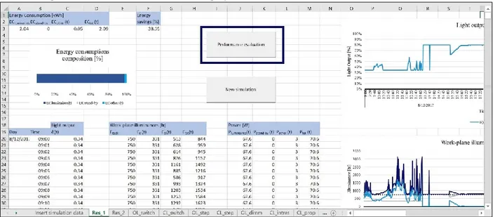
For these reasons, a new tool to evaluate DLCSs performances has been developed (DET- Daylight-linked control systems Evaluation Tool). It accepts as input data daylight availability values obtained by means of dynamic daylight simulation software. Then, based on them, it simulates the functioning of several control system typologies, accounting for different factors neglected by other available software. Specifically, the software is divided in two modules: the simulation module and the evaluation one. The former allows dynamically simulating DLCSs functioning, obtaining 𝐸̅𝑒𝑙(𝑡) values, the latter calculates Daylight Integration Adequacy (𝐷𝐼𝐴), Percentage Light Deficit (𝐿𝐷%), Percentage Intrinsic Light Excess (𝐼𝐿𝐸%) and Percentage Light Waste (𝐿𝑊%).
In the following paragraphs available simulation software and their limits are described, then DET is presented.
III.1. Today available software and their
limits
As it was mentioned in the II.1 Paragraph, the spread of dynamic daylight calculation has deeply changed the way to evaluate daylight.
The most accredited software in this field are those based on Radiance engine [81], specifically Daysim. It is a validated, RADIANCE-based daylighting analysis software, allowing the annual daylight availability in buildings to be modelled [77]. It contains a module to calculate energy savings connected to the use of different DLCSs. Users can divide the work-plane in different zones and define for each zone some control points. For each one of the control zones, users define the control strategy (switching or dimming) and the characteristics of the lighting system: Lighting Power, Standby Power and Ballast Loss Factor [69]. The software calculates daylight illuminances at the control points for each hour or fraction of hour (till 1 minute); evaluates the necessary luminaires light output to reach the required task illuminance at the control point and starting from the light output derives the
corresponding power absorbed by the lighting system. Finally, it infers consumptions and related savings based on power. This software most significant problem is that the control is based on the illuminance at the work-plane and not on photosensor detections. Moreover, the calibration procedure is neglected, so the control is simulated as an ideal one able to always perfectly integrate daylight, without determining excesses nor deficits.
The same simulation module is present in DIVA as well. DIVA is a highly optimized daylighting modelling plug-in for Rhinoceros based on Daysim engine [78]. However, the use of DIVA presents an additional problem: it does not allow performing sub-hourly simulations. As it was mentioned in Section 2 brief-time daylight oscillations can strictly affect dynamic daylight simulations functioning [16, 26, 67].
Mistrick developed at Penn State University a modified JAVA GUI for Daysim [77]. This tool can correctly model photosensors location and control algorithm settings, but it presents problems of compatibility with Windows operating system.
Rogers developed an Excel Macro called SPOT (Sensor Placement + Optimization Tool) [70, 82]. It is meant to help designers in defining control strategies, chose photosensors and establish their correct location. The tool contains a database of commercially available photosensors and can correctly model both spatial and spectral photosensor response and the calibration phase of different control typologies (switching, stepped and dimming ones). However, daylight modelling is simplified, and the software allows exclusively evaluating simple spaces characterized by square geometry.
Given that the mentioned software are all based on different calculation models, the use of a software or another, can provide different results in terms of achieved energy savings.
Doulos et al. [23] compared energy savings calculated by means of SPOT, and Daysim, referred to a dimming DLCS. They found that savings obtained with SPOT are 15% higher than those obtained by means of Daysim.
Williams et al. [83] evaluated that generally simulations overestimate actual savings for a percentage equal at least to 10%.
Given the weak points of the available software researches proposed alternative calculation models. Some studies focused their attention on the proposal of quick and simplified methods alternative to dynamic daylight simulations, useful especially in early design stages.
Krarti et al. [84] proposed a method to define energy savings achievable by means of dimming systems starting from the following parameters: the visible transmittance of the window glazing, the ratio of the window area to the daylit floor area, the ratio of the daylit floor area and the total floor area and two coefficients, a and b, depending on building location and control strategy. The algorithm was then extended by Ihm et al. [3]. They proposed an alternative method to evaluate a and b coefficients, accounting for the required task illuminance and the specific minimum light output of dimming systems.
Lo Verso et al. [85] developed a tool able to evaluate the electric lighting demand in the early design phases. It is based on two mathematical models, referred to a manual on-off switching and to a dimming DLCS respectively. The models were inferred from results of dynamic daylight
simulations studies performed with Daysim and referred to 828 different cases.
A simplified calculation method to evaluate the impact of the use of DLCSs on energy consumptions due to daylight is presented in the European standard EN 15193-1:2017 – Light and Lighting Part I: Energy requirement for lighting [86, 87] as well. It defines the LENI (Lighting Energy Numeric Indicator) representing the annual total energy for electric lighting per square meter in a building and proposes two calculation methods to calculate it: the complete and the rapid one. In the complete one it is proposed a methodology to evaluate the impact of Daylight responsive control systems. It is considered that the time during which the light is on is obtained by multiplying the occupation time of the building by reduction coefficients. One of these coefficients is the FD, accounting for daylight and being dependent on both the typology of the adopted control strategy and on the available daylight.
In this context, another interesting research field is represented by the use of artificial neural networks to predict the impact of daylighting and DLCSs on building energy consumptions [88-90]. Other studies proposed methods trying to overcome limits of dynamic simulation software. One of the most investigated issue is the way to correctly model the photosensor characteristics, i.e. spectral and spatial responses.
Doulos et al. [42] compared the illuminances detected by means of commercially available photosensors with those obtained by a sensor characterized by a spectral response matching the V(λ) function and they found that the shifts in detections varies in a systematic way. Based on these results, researchers proposed a parameter defined Photosensor Spectral Correction Coefficient (PSCC). It is the ratio of the illuminance registered by the specific photosensor and that measured by the ideal photosensor with a spectral response corresponding to V(λ). The use of PSCC could be used in simulations to obtain more reliable data.
Ehrlich et al. [91, 92] proposed a method to simulate the photosensor detections accounting for their spatial sensitivity starting from two different fisheye images obtained by means of Radiance.
Yoon et al. [93] proposed a method to simulate the spectral sensitivity. It consisted in modelling a
sphere with a diameter of 2.54 cm around the photosensor, assigning a “trans” material in Radiance and in defining a transmission function corresponding to the spectral response of the photosensor.
Other studies focused on lighting systems characteristics simulations.
For example [41, 64] proposed a method to simulate ballast dimming response functions. It consisted in measuring the relationship between control voltage and light output and light output and consumed power. Then best-fit functions describing this relationship were inferred with a regression process. These functions were then used to evaluate absorbed power as a function of the time. Specifically, the calculation phases were the following: daylight illuminances at the work-plane were evaluated by means of Daysim, the electric light requirement and the light output were derived starting from daylight illuminances; finally, from the light output the power was calculated by applying the above-mentioned functions.
Issues connected with the necessity to model the non-linear dimming curve of the luminaires, i.e. the curve relating light output and absorbed power are studied also in [94], where two different energy savings prediction models were verified by using real-time power consumption data.
III.2. DET description
DET is an Excel® macro, that, as it was anticipated in Paragraph III, can simulate the functioning of different DLCSs and evaluate their
performances. It is divided in two modules: the simulation tool and the evaluation one. The former module allows dynamically simulating the functioning of several DLCSs typologies, the latter calculates parameters to evaluate DLCSs performances.
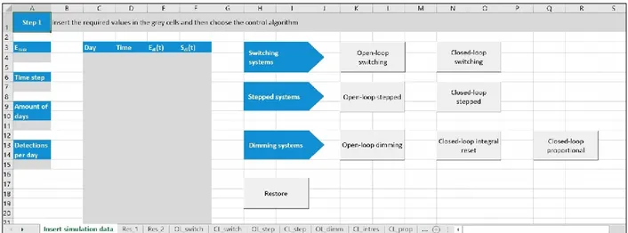
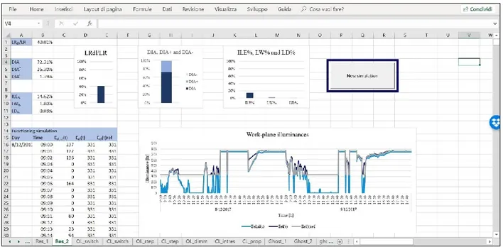
Basically, DET consists in a series of screens that users can easily navigate, moving from a section to another. The first screen (see Figure III.1), allows users inserting input parameters.
In more detail, in the A column the following data must be inserted in the specific cells:
• 𝐸𝑡𝑎𝑠𝑘, i.e. the task illuminance indicated by regulations, depending on the visual task performed in the studied environment;
• the time step of the simulation. It can be chosen thanks to a drop-down menu and it can be equal to one hour or one minute;
• the amount of simulated days;
• the number of data per day that were obtained by means of the simulation (for example considering a typical office scheduling, 8, if the simulation was hourly-based and 480 if it is minute-based).
Then, in the columns from C to F, users have to insert results of dynamic daylight simulations:
• date in C column; • time in D column;
• the values of daylight work-plane illuminances -𝐸𝐴,𝑑𝑙(𝑡)- in E column;