Stima e spazializzazione di attributi forestali tramite il metodo k-NN: distretto di Mocuba Mozambico

(1)

Dipartimento di Scienze dell'Ambiente Forestale e delle sue Risorse

Dottorato di Ricerca in Scienze e Tecnologie per la Gestione Forestale

e Ambientale

XVIII Ciclo

ESTIMATING AND MAPPING FOREST INVENTORY

VARIABLES USING THE K-NN METHOD: MOCUBA

DISTRICT CASE STUDY - MOZAMBIQUE

AGR/05 –Assestamento Forestale e Selvicoltura

Coordinatore: Prof. G. Piovesan

Tutor: Prof. P. Corona

Dottorando: Carla R. Pereira

(2)

Acknowledgements

This study was supported by the National Forest Inventory Unit within the Ministry of Agriculture of Mozambique which kindly provided the data used. To my colleagues from the Forest Inventory Unit I would like to express my special gratitude.

I thank my supervisor Prof. Piermaria Corona for his guidance and I would like to extend my immense gratitude to Dr. Paolo Calvani and Dr. Davide Travaglini for their patience and support with the k-NN and GIS softwares.

(5)

Abstract

Forest inventory covering vast areas provides a high number of variables and information that need to be processed from plot level to the overall inventoried area. The increasing availability of remotely sensed data has made possible to obtain a synoptic view over large areas, although with less accuracy than the field measurements. The introduction of georeferenced sample plots in forest inventories created the possibility of combining field data to satellite images, that is multisource forest inventories, and to expand the information from plot level to the overall image.

In this study, forest variables were estimated by means of Landsat ETM images and existing forest inventory field plots data. The study was carried out for Mocuba district in Zambézia province – Mozambique, characterized by typical african miombo forests with predominance of Julbernardia

globiflora and Brachystegia sp., covering an area of about 500 000 hectares. The non-parameteric

k-nearest neighbour (k-NN) estimator was used for estimating and mapping of three selected forest variables: total volume, commercial volume and forest density. The method has been applied successfully in temperate and boreal forests but only a few studies regarding species richness prediction can be found in the literature for tropical and sub-tropical regions.

To estimate the selected forest variables, k-NN parameters were firstly calibrated to the district data in order to determine the most appropriated distance type and number of neighbours. Results obtained are encouraging and in line with those mentioned in several literature and studies, mostly for Nordic countries. When the k-NN estimator and the central point/pixel value was used to estimate forest variables high relative errors were obtained, from 76 to 99%. When the average values of the pixels within sample plots with 30 meters buffer area was employed to estimate the forest variables the relative error dropped to 47 - 63%. Errors obtained are far higher than those allowed for forest inventory (usually less than 20%) and are not accurate enough for forest management purposes at district and concessions levels. However, the mapping of forest variables with a known error is a powerful instrument for strategic decision making. Forest variables estimates derived by the method can easily produced and used in areas where no other information exists or for non-sampled areas.

(6)

Abstract

Gli inventari forestale su vaste superfici forniscono un elevato numero di variabili ed informazioni che necessitano di essere processate dal livello di aree di saggio a quello della area complessivamente sottoposta all’inventario. La disponibilità crescente di immagini satellitari rende possibile ottenere una visione sinottica su ampie aree, ancorché con minor precisione rispetto alle misurazioni sul campo. L’introduzione di campioni georeferenziati negli inventari forestali ha offerto la possibilità di combinare dati di campo con gli immagini satellitari, ossia inventari forestali multisource, e di espandere le osservazione puntuale al suolo alla immagine complessiva.

Nel presente studio, le variabili forestali sono stimate per mezzo di immagini Landsat ETM e dati a terra del’ inventario forestal. Lo studio è stato condotto per il distretto di Mocuba, nella provincia della Zambesia - Mozambico, caratterizzata da foreste del tipico miombo africano con la predominanza di

Julbernardia globiflora e Brachystegia sp, che ricopre un’area di circa 500 000 ettari. Il algoritmo non

parametrico k-vicino più vicino (k-NN) è stato impiegato per la valutazione e la mappatura di tre variabili forestali selezionate: il volume totale, il volume commerciale e la densità forestale. Il metodo è stato in precedenza e con successo applicato in foreste temperate e boreali ma sono disponibili solo alcuni studi relativi alla previsione di ricchezza di specie nella letteratura sulle regioni tropicali e subtropicali.

Al fine di stimare le variabili forestali selezionate, i parametri k-NN sono stati calcolati per i dati del distretto per determinare il tipo di distanza e il numero di vicini più adeguati. I risultati ottenuti sono incoraggianti e in linea con quelli menzionati in una vasta letteratura ed in innumerevoli studi, soprattutto prodotti da Paesi nordici. Quando le stime è stata elaborata a livello di ciascun pixel, ne sono derivati errori relativi elevati, dal 76 al 99%. Quando i valori medi dei pixel dentro de l’unità de campionamento con 30 metri di “buffer” è stato utilizzato per derivare le variabili forestali, l’errore relativo si è abbassato a 47-63%. Gli errori ottenuti sono piuttosto elevati rispetto a quelli ammessi dagli inventari forestali (di solito inferiori al 20%) e non sono sufficientemente precisi per la realizzazione di piani di gestione forestale del distretto e delle concessioni forestali. Comunque, la spazializzazione di attributi forestali tramite k-NN con l’errore noto è un potente strumento per le determinazione di decisioni strategiche. Le stime delle variabili forestali ottenute con questo metodo possono essere facilmente prodotte e usate in aree dove nessuna altra informazione sia presente o per aree prive di campioni.

(7)

List of acronyms

BA - Basal area (m2_ha-1₎

Dbh - Diameter at breast height (cm) DN - Digital number

ETM - Enhanced thematic mapper FIU - Forest inventory unit Hc - Commercial height Ht - Total height

Mir - Middle infrared band MSS - Multi spectral sensors

NDVI - Normalized difference vegetation indice Nir - Near infrared band

RMSE - Root mean standard error SD - Standard deviation

TM - Thematic mapper Vt - Total volume (m3 _ha-1₎

Vc - Commercial volume (m3 _ha-1₎

List of figures

Figure 1 – The fate of incoming solar radiation Figure 2 – The electromagnetic spectrum

Figure 3 – Typical spectral response characteristics of green vegetation Figure 4 – Reflexive properties of a single leaf and canopies

Figure 5 – Typical spectral reflectances curves for vegetation, soil and clean water Figure 6 – Digital image

Figure 7 – Commercial volume map by species Figure 8 – Euclidean distance

Figure 9 – Study area location Figure 10 – Miombo distribution

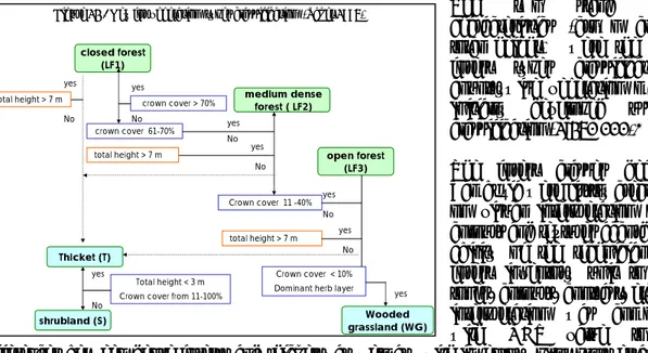
Figure 11 – Distribution of individuals by botanic family –Mocuba district. Figure 12 – Key for vegetation types classification

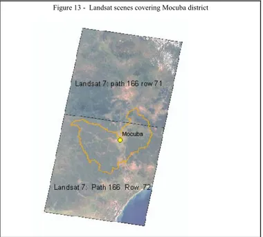
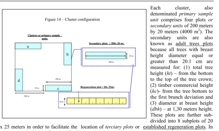
Figure 13 – Landsat scenes covering Mocuba district Figure 14 – Cluster configuration

Figure 15 – Digital earth model Figure 16 – Forest mask

Figure 17 – Training and validation plots for k-NN analysis Figure 18 – Training plots for pixel and plot level k-nn estimations Figure 19 – RMSE total volume versus k value- Euclidean distance

(8)

List of tables

TABLE 1 - LANDSAT BAND AND FEATURES ... 41

TABLE 2 - MAIN IMAGE COMPOSITES TYPES... 42

TABLE 3 - AVERAGE COMMERCIAL VOLUME FOR THE MAIN COMMERCIAL SPECIES –ZAMBÉZIA PROVINCE ... 48

TABLE 4 – AREA INVENTORIED BY FOREST TYPE – MOCUBA DISTRICT... 49

TABLE 5 - ESTIMATED FOREST VARIABLES FOR ALL FOREST AREA –MOCUBA DISTRICT ... 51

TABLE 6 - NUMBER OF CLUSTERS BY VEGETATION TYPE FOR MOCUBA DISTRICT ... 52

TABLE 7 - IMAGE METADATA... 53

TABLE 8 – IMAGE BANDS USED ON THE STUDY... 53

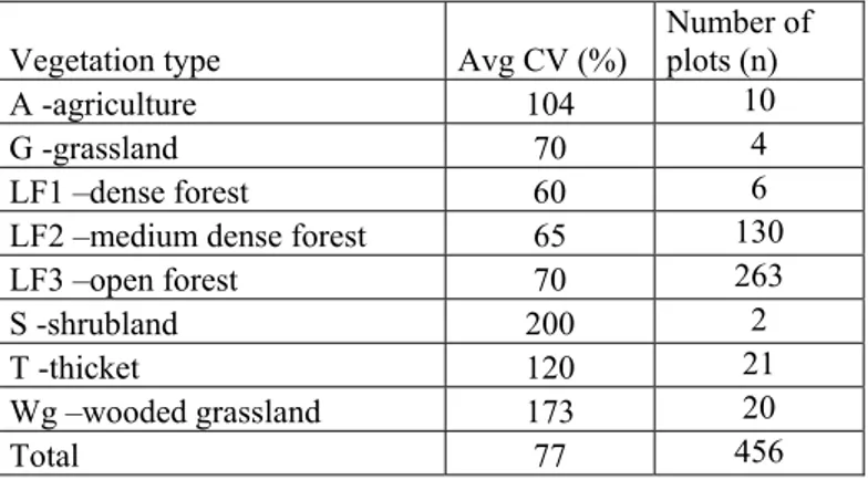
TABLE 9 – VARIATION COEFFICIENT BY PLOT FOR TOTAL VOLUME... 55

TABLE 10 – METHODOLOGICAL STEPS OF THE STUDY ... 57

TABLE 11 - DATA MINING AT PLOT LEVEL ... 57

TABLE 12 - STATISTICS SUMMARY OF TRAINING DATA ... 59

TABLE 13 – PEARSON CORRELATION COEFFICIENT BETWEEN FOREST VARIABLES AND MEAN DIGITAL NUMBER FOR PLOTS WITHOUT BUFFER (N=834) FOR ALL LANDSAT IMAGE 166072... 60

TABLE 14 - PEARSON CORRELATION COEFFICIENT BETWEEN FOREST VARIABLES AND MEAN DIGITAL NUMBER FOR PLOTS WITHOUT BUFFER FOR MOCUBA DISTRICT (N=711) ... 61

TABLE 15 - PEARSON CORRELATION COEFFICIENT BETWEEN FOREST VARIABLES AND MEAN DIGITAL NUMBER FOR PLOTS WITH 30 METERS BUFFER AREA FOR MOCUBA DISTRICT (N=711) ... 61

TABLE 16 - PEARSON CORRELATION COEFFICIENT BETWEEN FOREST VARIABLES AND DIGITAL NUMBER FOR TRAINING SUBPLOTS (25X20M) ... 62

TABLE 17 – REGRESSION ANALYSIS SUMMARY FOR TOTAL VOLUME AS DEPENDENT VARIABLE ... 62

TABLE 18 –REGRESSION ANALYSIS SUMMARY FOR COMMERCIAL VOLUME AS DEPENDENT VARIABLE ... 63

TABLE 19 – REGRESSION ANALYSIS SUMMARY FOR STOCKING AS DEPENDENT VARIABLE ... 64

TABLE 20 - SUMMARY OF BAND SELECTION... 65

TABLE 21 - BAND SELECTION ALTERNATIVES BASED ON K-NN CROSSVALIDATION ... 65

TABLE 22 – SELECTION OF BEST NUMBER OF NEIGHBOURS (K) FOR TOTAL VOLUME ESTIMATION ... 67

TABLE 23 – SELECTION OF BEST NUMBER OF NEIGHBOURS (K) FOR COMMERCIAL VOLUME ESTIMATION... 68

TABLE 24 – SELECTION OF BEST NUMBER OF NEIGHBOURS (K) FOR STOCKING ESTIMATION ... 69

TABLE 25 – SUMMARY STATISTICS BY VEGETATION TYPE AND STRATA... 69

TABLE 26 - PEARSON CORRELATION COEFFICIENT FOR STRATIFICATION BY VEGETATION TYPE : FORESTS AND MIXED FORESTS STRATA ... 70

TABLE 27 – TRAINING DATA AND K-NN PREDICTION FOR TOTAL VOLUME (M3 HA-1) ... 71

TABLE 28 – TRAINING DATA AND K-NN PREDICTION FOR COMMERCIAL VOLUME ( M3 _HA-1_{) ... 71}

(9)

TABLE 30 – ABSOLUTE RMSE OBTAINED WITH CROSS VALIDATION AND VALIDATION ... 72

TABLE 31 – ERRORS OF THE FOREST VARIABLES PREDICTION FOR PIXEL AND PLOT LEVEL ESTIMATES... 73

(10)

Definitions

Albedo: is the fraction of solar energy (shortwave radiation) reflected from the Earth back into space. Bit: is the short term for binary digit, which can take two possible binary values, 0 or 1. It is the smallest unit of storage and information within the computer.

Digital image: a digitally encoded record of spectral reflectance or emittance intensity for a selected object or area. A digital image is usually composed of one or more spectral bands. For each band, an individual pixel will have a digital number value (DN) to represent the intensity of spectral reflectance of the objects represented by the pixel.

Digital number: a positive integer representing the relative reflectance or emittance of an object in a digital image. For a 8 bit image the DN value lies in the range 0-255.

Electromagnetic energy: is a dynamic form of energy (visible light, radio waves, heat, X- rays, ultra-violet rays, microwaves,…) that is caused by the oscillation or acceleration of an electric charge. All natural and synthetic substances above zero degrees continuously produce and emit electromagnetic energy in proportion to their temperature. Electromagnetic energy passes through space at the speed of light in the form of sinusoidal waves. The wavelength is the distance from wavecrest to wavecrest. Electromagnetic spectrum: is a continuum of all electromagnetic waves arranged according to frequency and wavelength.

Forest types: a category of forest stands defined by composition, structure and age for management purposes. Saket (1995) defined the following forest types for Mozambique base on structural characteristics:

LF1 – lowland forests dense forests : vegetation with crown cover of upper stratum over 70 % with trees with more than 7 meters height and a herbaceous layer poorly developed.

LF2 – medium closed lowland forests: Vegetation composed of two to three strata. The crown cover of the dominant strata ranges from 40 to 70 percent. Trees are taller than 7 meters height and a moderate dense shrub layer is present with a sparse ground stratum. Herbaceous strata may or may not be present.

LF3 – Open lowland forests: vegetation with upper stratum crown coverage between 10 to 40 percent. The vegetation is composed of one to two tree strata associated with a moderate to abundant grass layer and a medium to dense shrub layer. A herbaceous stratum is present. T- thicket : vegetation with predominance of a tree layer and shrubs with crown cover percentage less than 10%. Is frequently the result of a degradation process following burning, overexploitation and overgrazing of forests.

S-shrubland: it is characterized by a low shrubby stratum (50cm to 3 meters) with occasional emergent trees with heights superior than 7 meters. Crown coverage percentage is variable (from 10% to high).

WG – wooded grassland: vegetation characterized by the predominance of a grass layer and a tree coverage less than 10% with variable tree height.

G – grassland: vegetation where predominates all types of herbaceous layer with some scattered trees. It is very difficult to distinguish and separate from agriculture.

(11)

A- agriculture: area where agriculture are being carried out within any of the other forest types, including grass covered lands previously used for agriculture and left as fallow.

Multisource forest inventory: uses various sources of geo-referenced data in addition to field inventory plots.

Pixel (combination of Picture & Element): is the smallest element of a display which can be assigned a colour.

Radiation: is the transfer of energy from one body to another in absence of an intervening medium. It is the only method by which solar energy cross space and enter the earth’s atmosphere.

(12)

1. Introduction

1.1 Remote sensing fundamentals

Understanding the basics of remote sensing is the prior step to understand the methodology used in this study, and the fundamentals of remote sensing science are generally described in this thesis chapter.

Remote sensing is initially defined as the collection of data about objects which are not in contact with the collecting device (Howard, 1991). The historical development of remote sensing has been divided into two general phases: (1) prior to 1960 when predominates the use of aerial photography and (2) after 1960 when started the use of satellites as the space platforms (Howard, 1991).

The evolution of remote sensing and its applications in forestry is connected not only to the evolution of data collection devices and platforms (balloons, aircrafts, satellite sensors and space shuttles) as well as to data processing, imagery analysis and presentation technology development. Consequently, remote sensing definition has evolved from “reconnaissance from a distance concept” to a more broad definition of reception, pre-processing, interpreting and latter analysis of data obtained from orbiting satellites (Campbell, 2002; Franklin, 2001).

There are several satellites types orbiting around the earth that provide a myriad of earth images. This study uses Landsat 7 ETM+ images and a general description of this satellite is given in this chapter. In general, satellites can be categorized according to its orbit into two main groups: (a) geostationary

satellites, that circle the Earth in a geo-synchronous orbit over the equator, that is, they orbit the

equatorial plane of the Earth at a speed matching the Earth's rotation allowing the Earth observation from the exact same place all the time and therefore continuously monitor a single position on the earth's surface. They give very coarse data (low spatial resolution > 2500 m/pixel) due to the fact that they usually orbit very far from earth (about 36 000 km above earth). There are more than 300 geostationary satellites mostly for meteorological and communications purposes, such as Meteosat (Europe), GOES (America), GMS (Japan/Australia), IODC (Indian Ocean), Skynet, etc. (b) polar

orbiting satellites, constantly circling the Earth in an almost north-south orbit, passing close to both

poles, sun synchronized, that is, covering each area of the world at a constant local time of the day known as local sun time. Their orbits are near-polar, covering the latitudes 82° north to 82° south of the equator with orbiting altitudes varying between 700 to 1500 km. Landsat and SPOT series of satellites have been the best-known polar-orbiters and have provided the most commonly used data in Mozambique.

100

% Incoming solar radiation

Absorbed by atmosphere and clouds Absorbed by earth’s surface 51% 19% 6% Refle cted by cloud s 20% Refle cted from surfa ce 4% Refle cted by earth ’s atm osph ere Emitted LW radiation from earth ( thermal remote sensing)

Figure 1 - The fate of incoming solar radiation

The underlying basis for most remote sensing methods is the measurement of the electromagnetic energy emanating from distant objects made of various materials, so that we can identify and categorize these objects by class or type, substance and spatial distribution. The electromagnetic energy is then captured by sensors which are classified in two categories: (a) active sensors when they transmit electromagnetic radiation and measure the reflection of this radiation such as the radar systems, and (b) passive

sensors that sense naturally available

energy such as the sun and do not output any form of electromagnetic radiation

(13)

towards the target area. The sun and the earth’s ambient temperature, (such as soil, water and vegetation) also known as the “terrestrial thermal infrared energy “, are the most common sources of radiant energy used in remote sensing (Lillesand and Kiefer, 1979).

Of the total income solar energy, 51% is absorbed at the surface, 19% absorbed by atmosphere and clouds and only 30% is reflected by the atmosphere, clouds and surface, that is, the albedo (Figure1). Therefore, the electromagnetic radiation captured by sensors is affected by two main mechanisms: (1) the atmospheric scattering /diffusion and absorption mechanisms and (2) the reflective characteristics of ground surface. When the radiant energy passes through the atmosphere, the amount of energy available to be detected by the sensor is affected by the atmospheric scattering, that is, the unpredictable diffusion of radiation by the existing particles in the atmosphere (gases, pollen, dust, smoke, water droplets…) that change the spatial distribution of the energy. On the other side, the atmospheric absorption is the process by which incident radiant energy is retained by the atmosphere constituents (water vapour, carbon dioxide and ozone). These gases absorb a portion of the radiant energy that is then re-emitted, usually at longer wavelengths, and some of it remains and heats the atmosphere;

When electromagnetic radiance from the sun, that is not absorbed or scattered in the atmosphere, hits the earth's surface three fundamental energy interactions take place: reflection, absorption and transmission. Reflection reflects light what we know as colour; i.e. chlorophyll in plants reflects green light; absorption takes place when the incident energy that is not reflected or transmitted is transformed into another form, such as heat or absorbed by chlorophyll in the process of photosynthesis; transmission takes place when energy propagates through a medium. The principle of conservation of energy points out that the incident energy is equal to the sum of reflected, absorbed and/or transmitted energy

On the other hand, when the electromagnetic energy hits the ground the reflective characteristics of the ground are different for each earth feature allowing us to distinguish different features on an image. Different materials reflect light of different wavelengths and by different amounts, known as spectral

reflectance curve or spectral signature. When viewing a remote sensing image on a particular band we

see a greyscale image showing the electromagnetic radiance received in that band from each point on the ground. Areas of higher radiance show lighter shades and areas of lower radiance show darker shades.

One advantage of satellite images when compared to aerial photographs is the possibility to capture non visible portions of the electromagnetic spectrum such as the Near Infra-Red wavelength. Wavelengths are measured in micron and the spectrum of waves is divided into sections based on wavelength. The shortest waves are gamma rays, which have wavelengths of 10-6_{microns or less. The longest} waves are radio waves, which

have wavelengths of many kilometres. The light used to "see" an object must have a wavelength about the same size as or smaller than the object (Figure 2). 10-5 ₁₀-2 Gamma X-ray UV Vi sib le R e fl e c ed IR 103₁₀2 T her ma l IR 104 ₁₀6 Mic ro w av e Radio Wavelength (µm)

Short wavelength long wavelength

High frequency low frequency

0.4 0.7

(14)

1.1.1 Spectral properties of vegetation

This property is of most interest for choosing the appropriate wavelength region for a particular application. The spectral reflectance curves for healthy vegetation manifest “peak and valley” configuration (Lillesand and Kiefer, 1979). Vegetation reflects much more energy in the near-infrared (0.8 to 1.4 microns) wavelength than it does in visible light (0.4 to 0.7 microns) as it is simply portrayed in figure 3.

The spectrum of plant leaves can be divided into three distinctive ranges:

1 - the range between 0.4 µm and 0.7 µm (visible band) is characterised by very low reflectance due to intense absorption of the incident radiation by pigments in the plant. On the visible portion of the solar spectrum, chlorophyll controls much of the spectral

response of the living leafs

(Campbell, 2002). Chlorophyll pigments absorb

at 0.43 - 0.45 µm (blue), and have an additional absorption band at about 0.65 µm (red) . There is a slight increase

in reflectivity around 0.55 µm band (visible green) because the pigments are least absorptive there.

Figure 3 - Typical spectral response characteristics of green vegetation.

Source:Crum, Shannon; http://www.rsunt.geo.ucsb.edu/rscc/vol2/lec2/2_2.html#21

Only 5-10% of the incident energy of the visible portion is reflected by a single leaf. This reflection makes leaves to appear green specially in the summer when the content of chlorophyll is at its maximum. During autumn/winter there is less chlorophyll content in the leaves and therefore they absorb less green wavelengths and reflect more red light making them to appear reddish or yellow.

2 – In the near infrared portion of solar spectrum (between 0.7 µm and 1.3 µm ) there is very little absorption and high reflectance. The reflectance of the leaf is controlled by the structure of the spongy mesophyll tissue, which causes multiple reflection of near infrared radiation at cell walls.

3 - The range between 1.3 µm and 2.6 µm (short infrared wavelengths) is characterised by pronounced minima. Leaf water content appears to control the spectral properties of the leaf, that absorbs most energy at these wavelengths as it is illustrated in figure 3. Reflectance of leaves is approximately inversely related to leaf liquid water content. This property can be used for identifying tree types and plant conditions (water stress) using remote sensing images

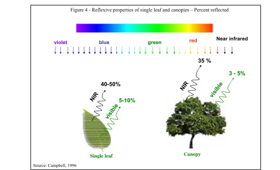
Vegetation canopies are composed of many separated leaves with several sizes, shapes, orientation and coverage of ground surface (Campbell, 2002). In a forest canopy upper leaves form shadows that cover the lower leaves and the overall reflectance is a combination of leaf reflectance and shadow. Campbell (2002) cited a study carried out by Knipling (1970), that illustrates that the canopy reflectance is less than the values observed in the laboratory for individual leaves. The reduction in reflectance for canopies is although much lower on the near infrared region than on visible spectra (figure 4).

(15)

Near infrared

NIR

visi ble

Figure 4 - Reflexive properties of single leaf and canopies – Percent reflected

5-10% 40-50% 35 % NIR visi ble 3 - 5% red green

Single leaf Canopy

blue

violet

Source: Campbell, 1996

The reflection of incident energy depends also on the vegetation cover. If vegetation cover is less than 100%, as it is in most of the cases for African savannas forests, then the reflectance properties of the underlying soil and water will also be also recorded by the remote sensor.

The difference of reflection in red band and NIR band is great for vegetation areas but insignificant for bare soil. Another important feature is that clear water reflects visible light only, so it will appear dark in infrared images (figure 5).

Figure 5- Typical spectral reflectances curves for vegetation, soil and clean water

Source:Crum, Shannon; http://www.rsunt.geo.ucsb.edu/rscc/vol2/lec2/2_2.html#21

Due to different reflectance curves the band ratioing (which underlies the vegetation indices construction) in the visible and infrared spectra can be a useful tool for imagery analysis.

Spectral vegetation indices

Spectral vegetation indices expresses the remotely sensed response observed in two or more wavebands as a single value that is related to the biophysical variable of interest (Foody et al., 2001 quoting Mather, 1999). They have been used since the late 1960’s and are continuously evolving and more than 50 vegetation indices have been developed for different applications and to account for noises in reflectance (Bannary et al., 1995). Healthy vegetation absorbs visible light, mostly red light, and reflects near-infrared. If a pixel has a large difference between NIR and Red band we assume that

(16)

the pixel probably represents an area covered by vegetation. A second assumption is that all bare soils in an image will form a line in spectral space (a red-near-infrared line for bare soils). This line is considered to be the line of zero vegetation.

Vegetation indices are classified accordingly to the orientation of lines of equal vegetation (isovegetation lines) in relation to the bare soils line: (a) slope indices, which consider that the isovegetation lines converge at a single point and the vegetation indexes measure the slope between the point of convergence and the red-NIR point of the pixel (e.g: NDVI, RVI); (b) perpendicular

distance indices, which consider that all isovegetation lines remain parallel to the soil line and measure

the perpendicular distance from the soil line to the red-NIR point of the pixel (eg. PVI). Some most used indices are below described. They can be classified as:

(1) Simple ratio vegetation index, such as the ratio vegetation index (RVI) attributed to Jordan (1969) ranges from zero to infinite and indicates the amount of vegetation by:

RVI = NIR band / Red band [eq.1]

(2) Normalized difference vegetation index, being the most widely used the Normalized Difference Vegetation Indice described by Rouse et al. (1973) though the concept was discussed by Kriegler et al. (1969) as : RED NIR RED NIR NDVI + − = [eq.2]

NDVI values vary from -1 to +1 . When there is no vegetation (zero percent cover) NDVI varies from 0 (snow) to 0.2 (organic black soil). If the NDVI it is between +0.2 to +0.3 correspond to shrubland/grassland area or open forests that are considered intermediate green cover. When green cover is between 30-40% the soil noise becomes at a maximum and decreases up to zero when a 100% green cover is achieved (NDVI between 0.6-0.8 indicates an area of tropical forests). A negative NDVI indicates an area of clouds, water or snow. Despite of the major weaknesses of NDVI (sensitive to variations in the background signal due to soil color, moisture and litter and influenced by atmospheric scattering) the widespread and strength of NDVI lies on its relative stability due to its power to reduce many form of noises such as: cloud shadows, topographic variations, illumination differences.

(3) Distance-based vegetation indices are designed to eliminate the effect of the background soil brightness and only detect the features of the vegetation cover based on Perpendicular Vegetation Indice (PVI) soil line concept which is a linear regression of the near infrared band against the red band for pixels of bare soil. PVI is the Perpendicular Vegetation Indice which was first described by Richardson and Wiegand (1977) as follow:

PVI = sin α (NIR) –cos α (red), [eq.3]

where α is the angle between the soil line and the NIR axis.

The vegetation indexes above described assume that there is soil line and a single slope in red-NIR space. But not all soils are alike and soils have different red-NIR slopes in a single image as well as changes in soils moisture cause noise to the vegetation reflectance. This problem is mostly detected when vegetation cover is low. Hence, other vegetation indexes were refined to account for the spectral reflectance properties of the underlying soil. The Soil Adjusted Vegetation Index (SAVI), designed by Huete (1988), acknowledges that the isovegetation lines are not parallel and that they do not all converge to a single point and that there is a simple radiative transfer from soil to vegetation. The index is based on a correction factor that varies from 0 for very high vegetation densities to 1 for

(17)

very low vegetation densities areas, and the standard value commonly used for intermediate vegetation density areas is 0.5 ) 1 ( L L red NIR red NIR SAVI + + + − = , [eq.4]

where L is a correction factor which ranges from 0 for very high vegetation densities to 1 for low vegetation densities.

This indice is slightly less sensitive to changes in vegetation cover than NDVI (but more sensitive than PVI) at low levels of vegetation cover.

(4) Indices that account for reducing atmospheric noise are also being developed. Kaufman and Tanre (1992) introduced the atmospheric corrections in the Vegetation indice called Atmospherically Resistant Vegetation Indice (ARVI). The red reflectance variable in NDVI was replaced with the term:

rb = red - gamma (blue - red), where the value of gamma is 1.0

rb NIR rb NIR ARVI + −

= , and ranges from -1 to +1. [eq.5]

Spectral relationships and forest inventory variables

Franklin (2001) mention that there has been several studies done to relate forest parameters to satellite data , and the relationships found are similar to those of aerial photographs:

• Increasing crown development is reflected by decreasing visible reflectance (darker tones); • Larger crowns absorb more light and reflect more the infrared;

The same author refers that remote sensors can only detect data that directly influence on the spectral response: illumination geometry (that is, target - sensor solar conditions) and amount of vegetation viewed from above (crown cover and canopy top reflection). In high resolution images (of 1 meter order) sensors detect several measurements for each tree, being each pixel records dependent on the part of the tree crown from which it was acquired. In Thematic Mapper Landsat images each ground resolution cell (nearly the size of a pixel) represent the average spectral response from several trees (Wallerman, 2003).

Remote sensing has proved useful for extracting land cover/use classes (forests versus non forests) and vegetation types/ecosystems defined by attributes detectable by remote sensors (for example based on crown cover percentage) and therefore for stratification and forest inventory planning (Franklin, 2001). Forest inventory variables such as dbh, commercial and total height, volume and so on, are considered second or third order variables, that is, can only be indirectly estimated through the existing correlations between crown size and closure and the indirect variable (Franklin, 2001).

Franklin (2001) cited a study carried out by Ripple et al. (1991) where the spectral response of Landsat TM data in homogeneous Douglas fir stands in USA was analyzed. It was found an inverse curvilinear relationship between the volume (m3 _ha-1_{) and many of the spectral bands (digital}

number), explained by the fact that young coniferous stands have a high reflectance due to a highly reflective presence of shrubs and herb layer while older stands with higher volume and shadows presented low reflectance.

(18)

On more heterogeneous and fragmented landscapes in Greek Mediterranean occurring patches of forested land mixed with agricultural farms and woodlands, stand volume and basal area show limited correlation with image data when compared to similar studies in uniform boreal forests due to many factors affecting the spectral response of vegetation (Mallinis et al., 2004). The following main factors affect the TM data ability to predict volume (Franklin, 2001):

• The homogeneity of forest stand. • The spatial scale.

• The range of volume to be investigated.

Although many studies were made in the past decade to identify the relationship between stand parameters and spectral response, the conclusions are site specific and the influence of different study areas characteristics on the spectral response is poorly understood and therefore conclusions can only be indicative. The following general conclusions can be extracted from the different studies (Lu et al,. 2004):

• visible bands are strongly related to biomass;

• middle infrared band has a strong negative relationship with stand timber volume;

• middle infrared bands are most sensitive to changes in forest volumes with reflectance in this spectral region being strongly related to canopy closure (Horler and Ahern, 1986);

• shadowing controls largely the forest canopy spectral response (Ardö, 1992);

• The near infrared wavelength reflectance present all kind of relationship with stand parameters: positive, negative or flat , due to shadowing and decrease of soil brightness; In boreal forests of Canada, Horler and Ahern (1986) concluded that the Landsat TM band 3 (red), TM band 4 (NIR) and TM band 5 (mid infrared) were the most appropriate bands for forest-cover-type discrimination.

Lu et al.(2004) studied the relationship between forest stand parameters and Landsat TM spectral responses in three sites of Amazonian basin and concluded that middle infrared band (TM5) was strongly correlated with forest stand parameters (biomass, basal area, mean diameter and height) and independent of biophysical environment.

1.1.2 Main characteristics of satellite sensors

Geostationary and polar orbiting satellites provide a large selection of remotely sensed data with respect to four parameters: (1) spatial, (2) temporal, (3) spectral and (4) radiometric sampling of earth surface. Its application and suitability depends on the resolution and extent of all 4 data parameters given by the satellite sensors. Resolution refers to the intensity or rate of sampling and is related to the smallest feature while extent refers to the overall coverage of a data set and is expressed as the largest feature.

Satellite remote sensing data captured by the sensors can be characterized by four main parameters: (1) Spatial resolution which refers to each individual pixel size and therefore expresses the level of

detail depicted in an image. In practice, represents a measure of the smallness of objects on the ground that may be detected as separate entities in the image. Pixel size is a function of the sensor characteristics (optics and sampling rate) and of platform (altitude and velocity) and vary in different satellite types and bands. The greater the distance between the satellite and earth the lower spatial resolution of image is obtained (for example, Quickbird = 450 km; Landsat = 705 km , Spot = 832 Km). Spatial extent refers to the overall image coverage also referred as swath width across the satellite orbit.

(19)

(2) Temporal resolution which indicates how often a sensor is acquiring an image for the same particular area. This imaging on a continuous basis at different times provide the possibility to monitor changes that take place on earth’s surface and are specially important if persistent clouds refrain the clear view of earth’s surface, short-lived phenomena are needed to be monitored and multi-temporal comparisons are required. Temporal resolution of a sensor depends on many factors, such as, sensors capabilities, swath overlap and altitude and is expressed as the number of days needed to repeat the orbit cycle. Temporal resolution varies from 2 images per day (NOAA), 1 image every 3 days (Quickbird) up to 1 image every 26 days (SPOT). Higher the temporal resolution there better chances of cloud free coverage. Temporal extent refers to the total period over which imagery is available, since satellites have an average life period from 3-5 years and can suffer some equipment disruption.

(3) Spectral resolution refers to the ability of a sensor to define fine wavelength intervals and is

expressed as the wavelength width. Spectral resolution is an important image feature since it contributes to distinguish different targets based on their spectral response in each band. Panchromatic photographs that capture one wide band (0.4 - 0.7 µm) are considered having low (coarse) spectral resolution, while Landsat is considered to have high spectral resolution since its sensors are sensitive to the individually reflected energy as blue, green and red wavelengths. More recently, advanced multispectral sensors also known as hyperspectral detect hundreds of very narrow spectral bands through the visible, near-infrared and mid-infrared portions of the electromagnetic spectrum (for example MODIS is considered to have a hyperspectral resolution (21 bands within the UV to NIR, 15 bands within the TIR, all with narrow bandwidths). Spectral

extent refers to the number and spectral range of channels in the image.

(4) Radiometric resolution refers to the ability of the sensors to discriminate very slight differences in

emitted or reflected energy and is expressed in terms of bits. Image data are displayed in a range of grey tones, with black representing a digital number of 0 and white representing the maximum or the saturation value (for example, 255 in 8-bit image). Higher radiometric resolution means more shades of grey, expressed by the number of the possible range of values a pixel may obtain. Landsat MSS detectors pixel range up to 128 levels (7-bit image), while Landsat TM pixel ranges up to 256 (8 bit image). Radiometric extent expresses the range of brightness values a sensor band is set up to capture and is expressed as the maximum brightness.

1.1.3 Characteristics of digital image

While aerial photography produces analogue images of the terrain, that is, an image represented by continuous variation in tone, images obtained by satellite remote sensing are digital. Digital images are reduced into numbers arranged in two-dimensional matrix (or raster data) of individual picture elements, known as pixels (figure 6). When a image is represented as numbers, brightness can be manipulated. Digital images have advantages over analogue film images because computers can store, process, enhance, analyze, and render images visible on a computer screen (Campbell, 2002).

Figure 6 - Digital image

Raw number

Column number

Digital number

(20)

Each pixel represents an area on the earth’s surface and stores two information: (1) the intensity value or pixel value and (2) location address numbers (given by its row and column number).

The address of a pixel is denoted by its row and column coordinates in the two-dimensional image. There is a one-to-one correspondence between the column-row address of a pixel and the geographical coordinates (e.g. Longitude, latitude) of the imaged location.

The intensity value, also known as the pixel value or grey level, represents the measured physical quantity such as the solar radiance in a given wavelength band reflected or/and emitted from earth’s surface. This value is normally the average value for the whole ground area covered by the pixel and is affected by the following main factors (Franklin, 2001):

• the spectral properties (reflectance, absorption, transmittance) of the earth surface targeted; • the illumination geometry and topographic effects;

• the atmosphere;

• the radiometric properties of the sensor, and

• the geometrical properties of the target (e.g., leaf inclination).

The intensity value or pixel value is digitised and recorded as a digital number. Due to the finite storage capacity, a digital number is stored with a finite number of bits (binary digits) which express the radiometric resolution of the image. The detected intensity value needs to be scaled and quantized to fit within this range of value. In a radiometrically calibrated image, the actual intensity value can be derived from the pixel digital number.

The use of digital number (DN) facilitates the visual display of image data and the design of instruments and data communication (Campbell, 2002). When doing analysis that compare relative brightness the use of digital numbers is satisfactory while for comparisons from scene to scene the use of radiances is more adequate since DN from one scene does not represent the same brightness as the same DN from another scene. Literature review shows that when using k-NN method to expand forest inventory variables from plot level to Landsat scenes, digital numbers directly extracted from the images data have been mostly used.

Digital remote sensing data is usually organized and stored into three main formats (Campbell, 2002) : (1) band interleaved by pixel (BIP) where data is organized in sequence values for each band by pixel; (2) band interleaved by line (BIL) where data is organized for each line on each band and (3) band sequential (BSQ) format where data is organized in sequence for each band treated as a separated unit.

1.1.4 Fundamentals of image processing

Once the raw remote sensing digital data has been acquired, it must be processed into usable information form. Computer digital image processing procedures can be categorized under the following main operations (Lillesand and Kiefer, 1979):

• image restoration that correct image distortions in order to truly represent the targeted object and involve mostly radiometric and geometric distortions corrections,

• image enhancement, that is the enhancement of image features through several techniques such as contrast and stretching in order to prepare the data to be easily interpreted, and • image classification, which deals with quantitative techniques that automatically interpret the

digital data and assign to each pixel an information category.

Image restoration, which comprehend radiometric and geometric corrections are generally done by

the image provider before delivering the data to the costumer and are also known as the pre-processing operations.

Landsat 7 ETM has onboard sensor radiometric correction for displacement of the scanner sweep with the forward movement of the satellite of ± 5%. Image based radiometric corrections are made to the

(21)

raw digital image data to remove for atmospheric effects from the image. The radiance values registered by the sensors do not directly reflect the ground reflectance because of the light scattering of a constantly changing atmosphere, also known as haze. Haze has an additive effect resulting in higher digital number values, decreasing the general contrast of the image. Haze is also wavelength dependent and is mostly pronounced in shorter wavelengths and negligible in near Infrared band. There are three main methods to estimate the atmospheric scattering: (a) image-based method which comprises the histogram minimum method and regression methods, (2) radiative transfer models and (c) empirical line model. Image-based methods are simple and do not require data about atmospheric conditions at the time image was taken like the radiative transfer models or field radiometers to measure the ground reflectance of a dark and bright target like in the empirical line method. The simplest atmospheric correction is performed by relating image information to pseudo-invariant reflectors, such as lakes, dark asphalt and rooftops (Franklin, 1991). Lillesand and Kieffer (1979) describe the histogram minimum method based on the assumption that pixels with the lowest digital number in the image dataset represent the features with nearly no reflectance (e.g., dark coloured rocks, water bodies) and therefore representing only the atmospheric scattering. If the average value of the lowest digital number pixels is subtracted in all dataset, the atmospheric scattering is eliminated and this operation is also called haze removal. On the other hand, the regression method is similar and applicable to dark pixels. The NIR pixel values are plotted against pixel values in the other bands. Regression methods best fit the line to data plotted and the resulting bias is assumed to represent the atmospheric radiance, and therefore subtracted from the all image.

The topographic effect is defined as the variation in radiance from inclined surfaces, compared with radiance from a horizontal surface, due to the surface orientation in relation to the light source and sensor (Franklin, 1991). The same author states that topographic corrections are more difficult to correct than haze removal and results are comparatively less certain.

Radiometric correction is specially needed if multitemporal images analysis are required as well as when more than one image is needed to cover a study area, or data is provided by different platforms

(Howard, 1991). By removing haze from the image, the brightness values across the set of images

are standartized making subsequent analysis easier and more reliable .

Geometric corrections are undertake to reduce the inaccuracy between the location coordinates of the targeted elements in the image data and the actual location coordinates on earth ground, so that the imagery will be as close as possible to the real world. This corrections are due to changes in altitude (topography), velocity of the satellite, eastward earth’s rotation and earth’s curvature (Howard, 1991 citing Berstein and Ferneyhough, 1975). Geometric correction involves the resampling of the image. This process consists of two main stages:

(1) The first stage concerns the selection of a set of ground control points (with known UTM coordinates) that are easily identified on the image. Usually the UTM coordinates are obtained from a topographic map in either digital (Digital Earth Models) or paper form and the image points must be matched to the ground control points. When considering the selection of ground control points it is important to consider two aspects: (a) the number of control points and (b) location of control points, which should be dispersed throughout the image with good coverage near the edges. Regarding the number of control points, Campbell (2002) quoting a study by Bernstein et al. (1983) recommended the use of 16 control points as a reasonable number since the accuracy of the ground control points may decrease as the number of control points increase because the analyst usually chooses the best points first. 16 ground control points can be considered acceptable if each of them can be located with an accuracy of one third of a pixel, considering as well that they are well distributed and the nature of landscape on the study area.

(22)

Two sets of data is obtained for each ground control point: their image coordinates and their true ground coordinates. These two sets of data are used to establish a mathematical relation through regression that interrelate the geographic and the image coordinates.

(2) The second stage consists on deciding the mathematical algorithm that will be used to assign the digital number to the newly geographic oriented pixel (usually in UTM coordinates). Three sampling algorithms are commonly used: nearest neighbour where the digital value for the corrected image pixel is derived from the digital number of the nearest pixel of the original image. This method is simple and does not change the original pixel values. The bilinear interpolation resampling algorithm uses the proximity-weighted for the 4 nearest pixels in the original image around to the output pixel location. This may result in changes to the original pixel value creating a new digital value in the geometric corrected image. The cubic convolution resampling algorithm which weighted averages the 16 closest pixels from the targeted pixel. This method results as well, in completely new pixel values but produces the sharpest image (Lillesand and Kiefer, 1979).

Image enhancement refers to procedures that simply transform the data into a more interpretable

form and are classified as point and local operations (Lillesand and Kiefer, 1979). Point operations refer to procedures that modify the brightness values of each pixel in an image data set independently while local operations modify the value of each pixel considering the context of the brightness values around it, or neighbourhood.

Image classification is the process of assigning pixels to classes, that in theory are homogeneous, that

is, those pixels within classes are spectrally more similar to one another than they are to pixels in other classes. Image classification is an important component of pattern recognition and image analysis field. There are many classification strategies that have been developed over the years but the most common ones can be referred as (Campbell, 2002): (a) point classifiers where each pixel is individually assigned to a class according to the several values measured in separate bands and (b) spatial or neighbourhood classifiers where groups of pixels are classified using both spectral and textural information. Classification has also been referred into two distinct types, according to the interaction with the image interpreter and field data (Campbell, 2002): (a) supervised classification which field data with known classes provide a guidance to the classification and (b) unsupervised classification where the image analyst has minimal interaction and classification is automated based on spectral classes that are uniform in respect to brightness.

When combining forest inventory sample data to pixels in the image to extrapolate the information at pixel level to the whole image, such as the one that is performed in this study, a supervised classification is used. The classifier is a computer programme or algorithm that implements a specific procedure for image classification. Supervised classification has been simply defined as the process of using samples of known identity (also known as training data) to classify pixels of unknown identity (Campbell, 2002). The main advantages of supervised classification are summarized as:

a) supervised classification allows the analyst to control the informational classes tailored to specific purposes or region. Unpredictable classes are not generated.

b) Supervised classification is tied to the geographic area from where the training data was collected.

c) Image analyst can detect errors in classification by using a validation dataset to determine the inaccuracy of classification.

Since supervised classification is based on training data which is collected with the aim of identifying a set of pixels that accurately represent spectral variation present in each class, the key characteristics of training areas are summarized as follows (Campbell, 2002) :

• Number of pixels: training areas should provide at least a total of 100 pixels for each class. • Size: small training areas are difficult to locate accurately on the image while too big training

(23)

optimum size of individual training samples since it varies according to the heterogeneity of each landscape and class.

• Shape: shape of training areas in not considered important.

• Location: training data must represent variation within the image and therefore must not be clustered in favoured classes or regions.

• Number: the optimum number depends upon several factors. A selection of a large number of training samples is recommended to allow for discard of some of them, as well as, the common sense indicates that is usually better to have many small training areas than use only a few large areas.

• Placement: training areas should be placed so that accurate location on image is allowed and should not encompass edge pixels of the class.

• Uniformity: it is considered the most important characteristic and data in each training area should exhibit a unimodal frequency distribution for each spectral band to be used.

1.2 Application of remote sensing in forest inventories and management

Forest inventories and field data collection can be supported either by airborne imagery (aerial photographs) or by spaceborn imagery (satellite images). Many authors review with several scales of details the application of aerial photographs for forestry science with emphasis on forest mensuration, timber cruising, forest management planning and monitoring, timber harvesting, roads planning, forest health and damages assessments (Loetsch and Haller, 1973; Lillesand and Kiefer, 1979). The use of aerial photography in forest inventories goes back to 1920’s when it was firstly used in Quebec boreal forests stock map preparation which combined aerial photo-interpretation and field checking plots (Howard, 1991, citing Wilson 1920). Today, the application of aerial photographs have been largely demonstrated either for both strategic inventories of large areas and for management purposes inventories of stand areas (Loetsch and Haller, 1973; Schreuder et al., 1993; Tuominen and Poso, 2001).

On the other hand, the launch of US Earth Resources Technological Satellite (ERTS-1) in 1972, latter renamed Landsat 1, marks the effective application of satellite remote sensing in forestry (Howard, 1991). Landsat satellites launched with a sun-synchronised and repetitive orbit (every 18 days) at nominal altitude of 900 km provide a fast and continuous information of large earth areas (around 3 million hectares per image) offering vast applications in other sciences than meteorological forecast. Literature cites several advantages of using remote sensing in forestry, particularly in large area surveys and for monitoring broad scale changes (continental, regional, national) in forest cover, density and land use (Loetsch and Haller, 1973; Howard, 1991). Boyd et al. (2002) citing DeFries and Townsend (1999) refer that remote sensing provides geographical referenced data for land cover mapping more accurate than data collected only by field surveys.

Multisource forest inventories employ various sources of geo-referenced data, in addition to field inventory plots in order to obtain more reliable estimates or estimates of smaller areas than when employing the pure field plot data only (Katila, 2004).

Besides the advantage of obtaining georeferenced data, the immense image archives from past decades of remotely sensed data acquired by earth resources satellite systems provide an unprecedented dataset to study land cover transformations over time and space (Boyd et al., 2002). When this archives are complemented with the increased resolution from satellite platforms and the reduction of image acquisition costs the use of remote sensing data for land management and monitoring purposes at various spatial scales is enhanced (Chen and Rogan, 2004).

Forest inventories use forest stratification into smaller, relative homogeneous forest types/stands in order to reduce variance and improve the precision of sample estimations. In statistical terms, forest

(24)

stratification should have minimized within-stratum variance while maximizing between-strata variance. In ideal terms, a forest type will be perfectly homogeneous and extremely different from the other defined forest types. In natural forests is not often the case since there are no clear borders between different forest types.

Forest stratification is often done by aerial photographs and more recently with the availability of satellite images, it has been done with the help of vegetation indexes and supervised image classification. Literature mention several advantages of using remote sensing in forestry inventories (Schreuder et al., 1993):

• Satellite images offer a synoptic view of a study area; • Satellite images cover large areas;

• Satellite image data can be digitally processed;

• Satellite image data is less expensive than aerial photographs.

Howard (1991) states that expectancy of Landsat applicability to forestry has been overstressed in relation to its operational role and that it is unlikely that satellite remote sensing will be able to provide the same quality and usable information as the aerial photographs.

Landsat satellite images analysis have successfully used for large area forest mapping and estimation of forest variables, forest changes detection over time and many other fields. However insufficient spatial resolution of Landsat images renders results less satisfactory for small areas inventories and for operative forest planning.

1.3 The use of remote sensing for forest inventories in Mozambique

Forest inventories in Mozambique are done for several purposes and scales. At national level, the first country based forest inventory was carried out in 1979/1980 pioneering the use of satellite images on national forest inventories. Forest inventory was based on the interpretation of MSS Landsat colour composite images from 1972-1973 covering the whole country (Malleux, 1980). The objective of national forest inventories is to produce statistically unbiased, reliable forest resources information for large areas for strategic planning, primarily by decision makers (Katila, 2004). The sampling over nationwide forest areas and the natural variability of forests require large amount of field plots to obtain reliable forest information. This requirement has to be traded-off with restricted budget for forest inventories and the on-growing demand for more variables and information to be collected. Foresters desperately look for tools to enhance the precision of estimations and to reduce costs of forest inventories.

The satellite images, which cover vast areas, fitted to that expectation, specially for countrywise forest inventories. The MSS landsat images used on the first Mozambican national inventory where utilized mostly to enhance forest stratification and as a tool for sampling design. Despite the use of satellite images, the first national inventory results were considered with low degree of precision due to limited time and human resources as well as due to the use of medium resolution satellite data (Saket, 1995). In Mozambique, satellite images where used as well, for forestry sector policy formulation on fuelwood and biomass energy subsector. 44 Landsat TM scenes from 1990-1991 covering the whole country where purchased to produce the country’s biomass assessment (ETC, 1987). These same images where latter used to update the 1980’s exploratory national inventory into two steps: (a) producing national forest map at the scale 1: 1 000 000 which did not gave enough details for development activities (Saket, 1995) and was followed up by (b) semi-detailed national forest types and land cover maps at 1:250 000 scale maps based on the 44 landsat MSS colour composed images (green, red and near infra-red bands).

(25)

These three works initiated the use of satellite images at nationwide level for policy and strategy formulation in the forestry sector. The inventory reports do not provide any information on the sampling error and estimations accuracy and results obtained where restricted by difficulties in obtaining field data because of the ongoing war and safety reasons. Some data such as tree species composition by forest types, diameter distribution for each species at district and provincial level , regeneration of natural forests and standing woody biomass where some of the non-existing information due to lack of comprehensive data gathering on the updating work of the national inventory (Saket, 1995). The same author recommended further detailed forest inventories based on representative sampling for the 10 provinces in the country to improve the existing information. This recommendation highlighted the need to obtain more detailed information at provincial level since that information was needed to backup forest management decisions (forest concessions and investments on forest plantations). The first attempt to obtain forest data at provincial level was done on the immediate years after the country’s independence in 1975 when two main large scale native forest inventories for strategic purposes where done in Niassa and Cabo Delgado provinces (Madebras et al., 1982, Silviconsult, 1984). Pancromatric black and white aerial photographs and topographic maps where the main tools for land use delineation, forest stratification and inventory planning on those days, but the war period restrict the use of the collected information and the inventory results.

After the country’s peace agreement, strategic forest inventories at provincial level funded by World Bank where initiated in Sofala and Cabo Delgado Provinces with the broad objectives of identifying the most suitable areas for forest concessions and to allow the elaboration of management plan models for forest concession areas. Recently, this work has been expanded to Zambezia and Inhambane provinces with Finnish cooperation funds.

All provincial forest inventories where heavily based on field data collection and as an immediate work result, forest inventory sampling design, field plot sizes, form and types, plot location, establishment and measurement procedures were rapidly standardized and field manuals produced in the country. Overall forest volume sampling error has been achieved within the acceptable limits, although in some cases when individual forest types are considered the sampling error per forest type and species increases and overcome the given limits.

Satellite images, vegetation and topographic maps used during the mentioned inventories have provided the key information for forest stratification and sampling design. While for Cabo Delgado and Sofala forest stratification was based on the visual interpretation of image tones and subsequently manual delineation of polygons, for Zambézia province the first stratification was based on a pilot inventory spectral classes given by the normalized vegetation index. A further stratification was based on a false composite image visual interpretation (band 1, 2 and 4) of forest polygons coupled with land use and cover maps as ancillary information.

Continuous variables such as volumes per forest type, volumes per tree species, tree diameters and heights were gathered through field plots while forest type boundaries and area compiled and updated through satellite image visual interpretation. Total forest growing stock is estimated based on the forest type areas and mean volumes per forest types. This traditional procedure has been applied either for strategic large scale forest inventories such as the national inventories and provincial forest inventories of Sofala, Cabo Delgado and more recently Zambézia and Inhambane, either to local forests with envisage of management plans elaboration for community forestry and forest concession areas. The present study estimates Mocuba district volume based on the provincial forestry inventory plots as reference plots for expanding the information through all district by mean of satellite image spectral data and explores its applicability to district level forest estimations and management.

(26)

1.4 Integration of spatial data and forest inventories

Traditional forest stand parameters inventories are expensive and difficult to obtain specially if vast and heterogeneous forest areas are considered. With the availability of remote sensing and the possibility of acquiring an overview of large areas through images several approaches have been studied to combine field data with satellite data. The methods can be classified into two main approaches (Franklin, 2001):

a) regression approach

Predicts the selected field variable using the remote sensing data as the dependent variable. The main constraints of using regression analysis to estimate forest parameters are (Foody et al., 2001):

(i) Linear regression analysis assume that exists a linear relationship between the remotely sensed data and the forest variables to be estimated. In reality most relations observed may be curvilinear.

(ii) Multiple regressions assumes that the independent variables (that is, the data acquired by the sensors in different spectral wavebands) are uncorrelated. This assumption is seldom satisfied since data in different spectral wavebands are very strongly correlated.

b) k-NN approach or reference sample plots (RSP) approach

Non-parametric k-NN estimates forest parameters based on plot data and corresponding pixel values to estimate the parameters at all pixels, without assuming a model that relates spectral variables and field variables.

The use of predictive methods were no data distribution and models are assumed, such as the nearest neighbour algorithm, may offer an alternative to integrate spatial data and forest inventory ground data.

(27)

2. Problem definition

Provincial forest inventories in Mozambique are made for strategic purposes and global monitoring of forest resources. Satellite images are mainly used during the planning phase to delineate the main forest types and separate forests from non-forest areas in order to obtain the most adequate sampling design for vast areas.

Traditionally, in Mozambique plotwise inventory has been used to derive the estimates for forest type level characterization.

The main problems of these forest inventory schemes can be summarized as:

1) Huge amount of information produced that requires long time for processing and report delivery. Zambézia forest inventory covered an area of about 4 million hectares. Data collection and processing required about 4 years to be completed and delivered to the general public and forest entrepreneurs. This is aggravated by the fact that the best forest areas are almost totally under logging activities with deficient registering (not georeferenced harvesting data). Forest inventory data produced becomes rapidly outdated.

2) The sampling design and intensity do not always allow the estimation of forest variables for a smaller units (such as districts or forest concessions) due to random distribution of samples and/or reduced sampling intensity in certain cases. In the recent Zambézia province forest inventory, results were calculated for aggregated district areas in order to obtain the desired level of accuracy of variables estimates. The applicability of provincial forest inventory data for forest management at local level (or even district level) may not be possible.

3) Mapping of continuous forest variables is not usually done due to the difficulties of spatializing plot level information to overall area based on sample plots. Therefore, the typical forest inventory main outputs is a forest type map complemented with figures and tables summarizing the characterization of forest types. Data as been considered difficult to understand and to relate to the ground information by the loggers and technicians. Figure 7 shows a map contained in the