https://doi.org/10.1007/s12667-020-00422-8
ORIGINAL PAPER
Short‑term stochastic movements of electricity prices
and long‑term investments in power generating
technologies
Carlo Mari1
Received: 12 August 2019 / Accepted: 23 December 2020 © The Author(s) 2021
Abstract
Modeling probability distributions for the long-term dynamics of electricity prices is of key importance to value long-term investments under uncertainty in the power sector, such as investments in new generating technologies. Starting from accurate modeling of the short-term behavior of electricity prices, we derive long-term sta-tionary probability distributions. Then, investments in new baseload generating technologies, namely gas, coal and nuclear power, are discussed. In order to com-pute the stochastic Net Present Value of investments in new generating technologies, the revenues from selling electricity in power markets as well as the costs which come from buying fuels at uncertain market prices must be evaluated over very long time horizons, i.e., over the whole lifetime of the plants. Starting from accu-rate short-term stochastic models of fuel prices in addition to electricity prices, we provide long-run probability distributions which are used to compute revenues and costs incurring during the whole lifetime of the plants. Five sources of uncertainty are taken into account, namely electricity market prices, fossil fuel prices (natural gas and coal prices), nuclear fuel prices and CO2 prices. Our evaluation model is calibrated on empirical data to account for both historical market prices and macro-economic views about future trends of electricity and fuel prices. The full probabil-ity densprobabil-ity of the stochastic Net Present Value is thus determined for each generation technology considered in this study.
Keywords Regime-switching stochastic processes · Mean-reversion · Probabilistic long-term forecasting · Stochastic net present value · Stochastic levelized cost of electricity
JEL Classification G31 · G32 · G33 · M21 · Q40
* Carlo Mari [email protected]
1 Introduction
Started at the beginning of the 1990s, the liberalization process of the electricity sector engaged several countries worldwide with the aim of transforming existing monopolistic markets into competitive markets. Such competitive markets were properly designed for allowing trades of electricity as a new commodity and were organized to discover equilibrium prices through demand and supply balancing. Electricity has, in fact, very peculiar characteristics [13]. It cannot be stored in an economically convenient way. Its transmission requires a constant balancing between injections to and withdrawals from the power grid. Moreover, electricity has a highly inelastic demand curve, strongly dependent on weather conditions (temperature, wind speed, precipitation, etc.). Supply is, in general, provided by low marginal costs generators but, in many cases, the mismatch between supply and demand, as for instance peaks in electricity demand, can be satisfied at very high costs [13, 50]. Given all this, it is not hard to understand how the liberalized marked interaction between demand and supply has dramatically increased the short-term volatility of power prices: shortages in electricity generation due to forced outages and/or grid congestions, peaks in electricity demand, fluctuations in hydroelectricity production, may result in unanticipated jumps in power prices and spikes of very high amplitude. These peculiarities have led to very erratic price dynamics not observed in any other commodity or financial market [48].
In the face of this, accurately modeling and forecasting electricity price dynamics becomes a crucial task for designing effective short-term trading strate-gies and long-term investments in power generating technolostrate-gies. Namely, at the corporate level short- and long-term electricity price forecasts are very important from the producer’s perspective [13, 53]. On one hand short-term price forecasts are of particular interest for defining bidding strategies [5] and scheduling pro-duction in order to maximize trading profits or hedge financial risk [4, 49]. On the other hand price forecasts on longer time horizons, ranging from a few years to decades, are of strategic importance for valuing investments in new generating technologies and for power planning decision making of energy companies and policy makers. Providing a link between accurate short-term modeling and long-term behavior of electricity prices is thus an important and necessary task.
Short-term price forecasting techniques are well developed in the literature, both for point and for probabilistic forecasting. A standard reference for price point forecasting is the in-depth review proposed by Weron [49]. Probabilistic forecasting consists of forecasting the whole price distribution or some related parts, as for example quantiles, at a time not too far in the future. Short-term probabilistic forecasting was recently reviewed by Nowotarski and Weron [40]. On the other side, long-run forecasting of electricity prices has not yet been investigated as much. This fact might be due to a limited understanding of the main drivers of the most important variables which affect electricity prices over long time horizons, as fossil fuel prices, environmental policies regarding CO2 emissions, technological changes, smart grid evolution, etc. [47]. Although some methods for long-term point forecasting electricity prices and their volatilities are
proposed in the literature (see, e.g., [1, 15]), papers on probabilistic forecasting methods, in which the probability density function of electricity prices is fore-cast, are few and they are mainly devoted to mid-term forecasting ranging from 1 month to 1 year [2, 3]. A review on probabilistic mid- and long-term electricity price forecasting was discussed by Ziel and Steinert [54]. In the same paper, the Authors proposed also a probabilistic approach to forecast electricity prices for several months up to 3 years. However, valuing investments in new generating technologies requires to take into account forecasts of revenues from selling elec-tricity at market prices and their volatilities for decades, i.e., over the whole life-time of the plant. The present paper aims to fill this gap in the literature by intro-ducing a new probabilistic approach to long-term forecasting in order to simulate revenues distributions over very long time horizons.
We propose a long-term forecasting methodology in which the long-run behavior of power prices is derived from the short-term dynamics. To this end, we will start from accurately modeling short-term random movements of electricity prices and we will end up to provide probability distributions in the long-run. In particular, we discuss three short-term stochastic models. In the first model, which we will name ‘Model 1’, the dynamics of electricity prices is described by a mean-reverting dif-fusion process. In the second model, i.e., ‘Model 2’, a mean-reverting jump-diffu-sion process is used to describe the dynamics of prices. Finally, in the third model, i.e., ‘Model 3’, the dynamics of electricity prices is described by a mean-reverting two regime-switching Markov process. Mean-reversion is a very relevant feature of the electricity price behavior observed in power markets. First, it is responsible for reducing prices after a spike has occurred; second, it forces the stochastic compo-nent of prices to fluctuate around some long-run mean, driving probability densities toward stationary long-run distributions. By the use of mean-reversion, the short-term dynamics can be connected to the long-short-term behavior of power prices. Moreo-ver, these models can be calibrated on historical data and can include a structural component in terms of forward looking information based on macroeconomic views about the future long-term evolution of electricity prices. In this way, the proposed approach develops a robust link between accurate short-term modeling and long-term behavior of electricity prices. This is one of the novelty aspects of the present paper and the first main contribution to the literature.
Long-run forecasting is an important topic of research. When an electricity com-pany plans to build new power plants, it needs long-term revenues and generation cost forecasts over the whole lifetime of the plants, basing its decision-making on some long-term metrics as, for example, the Net Present Value (NPV) of the invest-ment [24]. The NPV criterion is a widespread method suitable for long-term eval-uation [31, 45] that takes into account revenues from selling electricity in power markets and costs incurred during the whole lifetime of the plants. In addition, the stochastic NPV theory, which attributes to the NPV a probability distribution, pro-vides a powerful tool to perform risk analysis of investments [45].
As a second contribution to the existing literature, we discuss an evaluation scheme for risky investments in new baseload generating technologies, namely fossil fuel (gas and coal) power plants and nuclear power plants, based on the stochas-tic NPV as a long-term metric. The stochasstochas-tic NPV is computed under accurate
modeling of the stochastic dynamics of the main factors affecting the profitability of the investment. In this regard, five sources of uncertainty are taken into account, namely electricity market prices, fossil fuel prices (natural gas and coal prices), nuclear fuel prices and CO2 prices. Market based CO2 pricing schemes (like the European Union Emissions Trading Scheme, EU-ETS) generate volatility in CO2 prices [14, 38] through the interaction between demand and supply, thus introducing a new source of uncertainty which must be taken into account for valuing invest-ments in power generation technologies [20]. These factors are the main financial risk sources in the electricity sector [15, 26]. Since the analysis is limited to base-load technologies, quantity uncertainty has a minor effect and it is not taken into account. Regarding the nuclear source, we do not consider here the financial risk due to the social acceptance of this technology. The reason is that we assume that the investment evaluation is performed in a case in which the nuclear power genera-tion is a well accepted technology. Although in principle construcgenera-tion costs could be stochastic, especially for nuclear power plants [27], we do not consider here this possibility. However, the model can be extended to account for uncertainty in all types of costs.
The novelty of this approach is to provide a model to value investments in new baseload generating technologies in a stochastic framework in which random move-ments of electricity and fuel prices are accurately modeled both in the short- and in the long-term. The starting point of our analysis is modeling the short-term behavior and then investigate the long-term limit in order to compute stochastic revenues and costs during the whole lifetime of the plants. Regarding the electricity price dynam-ics, we use the regime-switching Model 3 that better describes the random move-ments of electricity prices observed in real markets with respect to Model 1 and Model 2 (as it is will shown in the following). From the costs side, fuel prices too are modeled according to well defined stochastic processes. In particular, since gas market prices exhibit mean-reversion and jumps, we use a mean-reverting jump-dif-fusion model to capture the features of the short-term dynamics of gas prices. Coal and nuclear fuel prices do not show mean-reversion and we assume that their time evolution are both described by a Geometric Brownian Motion (GBM). As a further source of uncertainty, we will consider the possibility to include CO2 costs into the analysis. CO2 prices will be modeled according to a GBM. As suggested in the lit-erature, the long-run analysis of investments in the power sector must integrate his-torical data and future trends in market prices, including expert evaluations of future regulations and forthcoming technologies [19]. The evaluation model we propose can be calibrated on historical data on market prices and can incorporate a structural component in terms of macroeconomic views about future trends of electricity and fuel prices. This approach allows us to determine the probability density of stochas-tic NPVs of new generating technologies and to perform risk analysis of investments in capacity expansion. The empirical analysis, based on cost data of new generating technologies collected from the ‘Annual Energy Outlook 2019’ [9] reveals that, with the exception of the gas generation, both coal and nuclear power generation show a negative expected NPV. This is an important result which can be useful for both investors and policy makers in their efforts to plan capacity expansion and future power system configurations. This is the third main contribution to the literature.
It could be interesting to relate our approach to more structural approaches to long-term price setting and forecasting. For example, in the model proposed by Oliveira and Costa [41] a fictional microeconomic dynamics drives the market to an equilibrium, which is reached by groping and mutual learning by part of the market agents. Since the dynamics is fictional, no information can be given about the real dynamics which will go on inside the period studied. In the model proposed by De Vries and Heijnen [8], the specific aim is understanding how the dynamics of elec-tricity generation capacity growth can be stimulated and controlled in time, within a long-term horizon. In this case, demand and supply changes are matched in time under different regulatory and legislation schemes, and under demand growth uncer-tainty. Together, these two approaches can be taken as examples of possible ways to tackle with one of the most important facts behind long-term price valuation. Price forecasting on long time horizons means taking into account a capacity expansion problem and its impact on prices [6], especially in the presence of variable renew-able energy (VRE) sources [52]. It is certainly not easy to include this feature into long-term forecasting models. In any case, making an econometrics of prices emerge from matching demand with supply is in the end deeply linked to our approach. In a different but twin way, the stochastic NPV assessment tries to model a decision process under uncertainty, yet without directly coping with the microstructure of the power market. In our approach, the effects of the microstructure are included in the phenomenology of historical power and fuel prices, and we indirectly include it by calibrating the model on empirical data related to historical market prices over long time horizons and on macroeconomic forward looking views about future trends of electricity, fuel and CO2 market prices.
The paper is organized as follows. Section 2 discusses the short-term dynamics of electricity prices. Some models are introduced and estimated on historical data from Palo Verde and PJM markets. In Sect. 3, the long-term behavior of electricity prices is investigated, and stationary probability distributions are derived and discussed. Section 4 introduces the stochastic NPV metric and its link with the stochastic Lev-elized Cost Of Electricity (LCOE). Sections 5 and 6 concern the stochastic mod-eling of revenues and costs respectively. In Sect. 7, a stochastic NPV based analy-sis of investments in new generating technologies is provided. Section 8 concludes. Finally, “Appendix ” provides some technical results about the time evolution of central moments in the jump-diffusion model.
2 Modeling electricity price dynamics
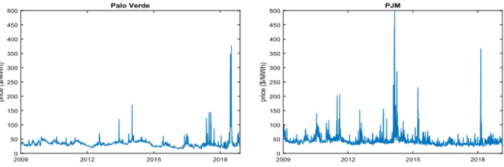
Figure 1 depicts the time series of daily electricity prices observed between January, 2009 and December, 2018 at the two US power markets of Palo Verde (US South-west region) and PJM (US Northeast region). Daily prices are obtained as weighted averages of the 24 hourly market prices and are expressed in nominal dollars per megawatthour ( $/MWh). These electricity price time series are available at www. eia.gov/elect ricit y/whole sale and are freely downloadable.
Looking at Fig. 1, we note that electricity prices follow a very erratic dynam-ics characterized by high volatility, jumps and pronounced spikes. Moreover,
multi-regime dynamics can be observed. In normal stable periods, prices fluctu-ate around some long-run mean; in turbulent periods prices experience jumps and short-lived spikes. After a jump or a spike has occurred, a mean-reversion mecha-nism forces back prices to fluctuate around some long-run mean. Accurate modeling power price dynamics means to take into account all these features.
Several continuous-time models for electricity prices were proposed in the litera-ture. Since the seminal paper by Lucia and Schwartz [30], in which a mean-reverting diffusion process was proposed to model the power price dynamics at the Nord Pool market, the literature on this topics has grown exponentially. Mean-reverting jump-diffusion processes and mean-reverting regime-switching models were extensively used to accurately describe the jumpy and the spiky behavior of electricity prices observed in power markets. In this section we focus on three models of these types, namely a mean-reverting diffusion model, a mean-reverting jump-diffusion model, and mean-reverting two regime-switching model.
Let us denote by P(t) the daily price at time t of one MWh of electricity, and by
s(t) =ln P(t) its natural logarithm. We assume that s(t) is a linear superposition of a deterministic component, f(t), possibly accounting for trend and seasonality, and a random component, x(t), namely
Since electricity prices may be higher in winter time and in summer time, we express the deterministic component as
to describe the semiannual periodicity. A linear trend is included to account for expected inflation and possibly for a real escalation rate of power prices (positive or negative). The parameter 𝜏 denotes the average number of observations per year. One can estimate the seasonal component parameters bj ( j = 0, 2, ⋯ , 5 ) by fitting
f(t) to market data using Ordinary Least Squares (OLS) techniques. Table 1 depicts the parameters estimates obtained in the Palo Verde and PJM power markets.
Figure 2 shows the time series of stochastic log-returns (hereinafter, log-returns) obtained as daily changes of the random component x(t), at Palo Verde market (left (1) s(t) = f (t) + x(t). (2) f (t) = b0+ b1t + b2cos(b3+2𝜋t 𝜏 ) + b4cos(b5+ 4𝜋t 𝜏 ), 2009 2012 2015 2018 price ($/MWh ) 0 50 100 150 200 250 300 350 400 450 500 Palo Verde 2009 2012 2015 2018 price ($/MWh ) 0 50 100 150 200 250 300 350 400 450 500 PJM
Fig. 1 Historical behavior of power prices at Palo Verde market (left) and at PJM market (right) since January, 2009–December, 2018
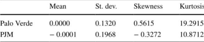
panel) and at PJM market (right panel). Descriptive statistics of log-returns are dis-played in Table 2.
As mentioned in Sect. 1, and as it can be seen also in the figure, interplay between demand and supply generates a lot of volatility in nowadays power markets. Log-returns show large fluctuations with jumps and spikes, and non-normal, lepto-kurtic empirical distributions. With the aim of capturing the features of log-returns observed in these markets, we discuss now three continuous-time stochastic models for the dynamics of x(t), called, respectively, Model 1, Model 2 and Model 3. The main features of these models are described below.
2.1 Model 1
In Model 1, the dynamics of x(t) is described by the following mean-reverting diffu-sion process,
where 𝛼0 is the mean-reversion parameter, 𝜎0 is the volatility, and w0(t) is a Wiener process. Although this model captures the mean-reverting behavior of power prices, (3)
dx(t) = −𝛼0x(t)dt + 𝜎0dw0(t),
Table 1 Parameter estimates of the deterministic component
b0 b1 b2 b3 b4 b5 Palo Verde 3.6022 −0.0933 × 10⁻³ − 0.1553 − 0.8087 0.1065 − 0.5117 PJM 3.9192 −0.1364 × 10⁻³ − 0.0196 0.5443 0.0930 − 0.6625 2009 2012 2015 2018 daily log-return -1 -0.5 0 0.5 1 1.5 Palo Verde 2009 2012 2015 2018 daily log-return -1.5 -1 -0.5 0 0.5 1 1.5 PJM
Fig. 2 Historical behavior of log-returns at Palo Verde market (left) and at PJM market (right) since Jan-uary, 2009–December, 2018
Table 2 Descriptive statistics of
log-returns Mean St. dev. Skewness Kurtosis
Palo Verde 0.0000 0.1320 0.5615 19.2915 PJM − 0.0001 0.1968 − 0.3272 10.8712
it is not able to account for jumps and spikes. This limitation can be overcome by modeling power price dynamics with a jump-diffusion process.
2.2 Model 2
In Model 2 the dynamics of x(t) is described by a mean-reverting jump-diffusion pro-cess of the form
where q(t) is a Poisson process with constant intensity 𝜆 . In Eq. (4) the random jump amplitude J is distributed as a Gaussian random variable with zero mean and stand-ard deviation 𝜎J , i.e. J ∼ N(0, 𝜎J2) . We assume that the Wiener process, the Poisson
process, and the jump amplitude are mutually independent processes. We remark that the zero mean jump amplitude was chosen according to the observed low values of the skewness present in the data (see Table 2). Nevertheless, the proposed analy-sis is general and can be extended in a straightforward way to include jumps with arbitrary probability distributions (see “Appendix ”).
2.3 Model 3
Model 3 consists of a regime-switching process with two regimes. Regime-switching processes add a further degree of freedom to the description of the dynamics of elec-tricity prices. In our specific, they allow us to combine in one model periods of steady dynamics and of jumpy dynamics, depending on the realization of a stochastic two-valued latent state variable of the system. We can thus make use of two different state-dependent mean-reversion rates and include stochastic volatility. Model 3 is character-ized by the following process,
The dynamics of the base regime (first line of Eq. 5) is described by a mean-revert-ing diffusion process in order to account for the motion durmean-revert-ing stable periods. In contrast, the dynamics of the jumpy regime (second line of Eq. 5) is described by a mean-reverting jump-diffusion process. As in the two previous models, w0(t) and
w1(t) are Wiener processes and q(t) is a Poisson process with constant intensity 𝜆 . In Eq. (5) the random jump amplitude J is distributed as a Gaussian random variable with zero mean and standard deviation 𝜎J , i.e., J ∼ N(0, 𝜎J2) . We assume that the
Wiener processes, the Poisson process, and the jump amplitude, are mutually inde-pendent processes. The switching between regimes is driven by a hidden Markov process characterized by the following transition probability matrix,
(4) dx(t) = −𝛼0x(t)dt + 𝜎0dw0(t) + Jdq(t), (5) dx(t) ={ −𝛼0x(t)dt + 𝜎0dw0(t), −𝛼1x(t)dt + 𝜎1dw1(t) + Jdq(t). (6) 𝜋 =( 1 − 𝛾dt 𝜂dt 𝛾dt 1 − 𝜂dt ) ,
where 𝛾dt denotes the transition probability of a switch from the base regime to the turbulent regime in the infinitesimal time interval [t, t + dt] , and 𝜂dt is the probabil-ity of the opposite transition.
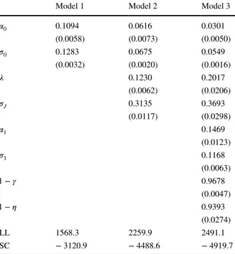
All these models were estimated on market data by maximum likelihood using the Euler discretization with time step 𝛥t equal to 1 day. In the case of Model 3, the Hamilton filtering technique [17, 18] was used. Estimation results are depicted in Table 3 for the Palo Verde market, and in Table 4 for the PJM. For each market, the parameters estimates, the log-likelihood (LL), and the value of the Schwartz crite-rion (SC) are reported.
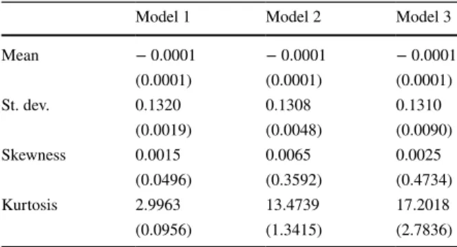
As it can be read from the last line of these tables the empirical analysis reveals that the regime-switching model describes the dynamics of electricity prices better than diffusion and jump-diffusion models. The Schwartz criterion indicates that the presence of jumps in the dynamics enhances the fit. Moreover, the added degrees of freedom coming from multiple mean-reversion rates and volatilities (i.e., for the base and the turbulent regime), makes regime-switching models more suitable to describe the dynamics of electricity prices observed in real markets [32, 37]. As expected, the mean-reversion parameter as well as the volatility parameter are lower in the base regime with respect to the turbulent one. The statistical analysis of simulated trajectories confirms that regime-switch-ing models offer an interestregime-switch-ing agreement with market data. Tables 5 and 6 dis-play some parameters computed from simulated log-returns time series. Such val-ues are computed averaging over ten thousands randomly generated paths using, respectively, Palo Verde and PJM estimates to be compared with the statistics
Table 3 Palo Verde estimation results
Standard errors are between parentheses
Model 1 Model 2 Model 3
𝛼0 0.1094 0.0616 0.0301 (0.0058) (0.0073) (0.0050) 𝜎0 0.1283 0.0675 0.0549 (0.0032) (0.0020) (0.0016) 𝜆 0.1230 0.2017 (0.0062) (0.0206) 𝜎J 0.3135 0.3693 (0.0117) (0.0298) 𝛼1 0.1469 (0.0123) 𝜎1 0.1168 (0.0063) 1− 𝛾 0.9678 (0.0047) 1− 𝜂 0.9393 (0.0274) LL 1568.3 2259.9 2491.1 SC − 3120.9 − 4488.6 − 4919.7
from original data shown in Table 2. We can observe that the statistical analysis of simulated trajectories shows an interesting agreement with market data in the case of Model 3.
We conclude this section by noticing that Palo Verde and PJM markets are characterized by very different values of the mean-reversion rate. In all the mod-els which we discussed, mean-reversion parameters estimated on Palo Verde mar-ket data are lower than those estimated on PJM marmar-ket data. As we will see in the following sections, this fact has important consequences on the long-run behavior of electricity prices.
Table 4 PJM estimation results
Standard errors are between parentheses
Model 1 Model 2 Model 3
𝛼0 0.2075 0.1684 0.1213 (0.0092) (0.0123) (0.0077) 𝜎0 0.1863 0.1182 0.0968 (0.0034) (0.0050) (0.0059) 𝜆 0.1589 0.1856 (0.0104) (0.0158) 𝜎J 0.3624 0.4317 (0.0325) (0.0250) 𝛼1 0.2643 (0.0234) 𝜎1 0.2022 (0.0059) 1− 𝛾 0.9422 (0.0051) 1− 𝜂 0.9057 (0.0051) LL 662.9 988.2 1142.6 SC − 1310.1 − 1945.0 − 2222.5
Table 5 Statistics of simulated path log-returns obtained using Palo Verde estimated parameters
Standard deviations are between parentheses
Model 1 Model 2 Model 3
Mean − 0.0001 − 0.0001 − 0.0001 (0.0001) (0.0001) (0.0001) St. dev. 0.1320 0.1308 0.1310 (0.0019) (0.0048) (0.0090) Skewness 0.0015 0.0065 0.0025 (0.0496) (0.3592) (0.4734) Kurtosis 2.9963 13.4739 17.2018 (0.0956) (1.3415) (2.7836)
3 Long‑term evolution of electricity prices
The long-term behavior of electricity prices can be investigated by studying the time evolution of the central moments of log-price distributions. Central moments are defined by
where 𝜇(t) = E[x(t)] denotes the expected value of the random variable x(t). In both Model 1 and Model 2 if x(0) = x0 is the initial condition of the process, 𝜇(t) is given by
In these two models, closed form solutions for central moments can be found. In particular, odd central moments are zero and the first two even moments are given by and in Model 1, and by and (7) Mn(t) = E[(x(t) − 𝜇(t))n], (8) 𝜇(t) = x0e−𝛼t. (9) M2(t) = 𝜎2 2𝛼 ( 1 − e−2𝛼t ) , (10) M4(t) = 3[ 𝜎2 2𝛼 ( 1 − e−2𝛼t )]2 = 3M2(t)2, (11) M2(t) = 𝜎 2+ 𝜆𝜎2 J 2𝛼 ( 1 − e−2𝛼t ) ,
Table 6 Statistics of simulated path log-returns obtained using PJM estimated parameters
Standard deviations are between parentheses
Model 1 Model 2 Model 3
Mean 0.0000 0.0000 0.0000 (0.0001) (0.0001) (0.0001) St. dev. 0.1968 0.1950 0.1970 (0.0028) (0.0056) (0.0084) Skewness − 0.0018 − 0.0022 − 0.0053 (0.0462) (0.1961) (0.2431) Kurtosis 2.9943 7.7619 9.5101 (0.0972) (0.7079) (1.2655)
in Model 2. The proofs of the above equations as well as the proofs of the formulas presented in this section are provided in A.
It is well known that x(t) are normal variables for t > 0 in Model 1 [16], but they are not normal in Model 2, as it can be verified by the value of the kurtosis which is different from 3. In the limit t → ∞ , central moments converge toward stationary values that can be computed by using the recursive relationship
in Model 1, and by
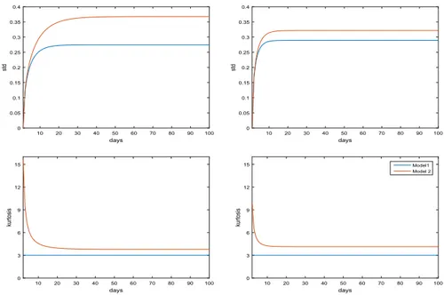
in Model 2. The stationary value of the kurtosis is K = 3 in Model 1, and
in Model 2. Figure 3 depicts the time behavior of standard deviation and kurtosis, computed with estimated parameters at Palo Verde and PJM markets for both Model 1 and Model 2.
In market data, probability distributions tend to be stationary in a few tens of days. After this time interval, the process random variables x(t) and x(s) become identically distributed for any time t and time s. The speed of convergence to the sta-tionary distribution depends, of course, on the mean-reversion parameter. The con-vergence is, therefore, faster for PJM market prices. Moreover, random variables x(s) and x(t) ( t ≥ s) become uncorrelated in a few tens of days. To show this, we notice that the autocorrelation function can be computed in a closed form in both models and reads,
in Model 1, and
in Model 2. For large s, i.e., after some tens of days, the autocorrelation function becomes stationary in both Model 1 and Model 2. It depends on the time difference,
s − t , with a correlation coefficient which decreases exponentially,
(12) M4(t) = 3𝜆𝜎 4 J 4𝛼 ( 1 − e−4𝛼t ) + 3M2(t)2, (13) M2n= 2n − 1 2𝛼 𝜎 2M 2(n−1) (14) M2n= 2n − 1 2𝛼 𝜎 2M 2(n−1)+ 𝜆 2n𝛼 n ∑ k=1 (2n)! 2kk!(2n − 2k)!𝜎 2k J M2(n−k) (15) K =3 + 3 𝜆𝜎 4 J 𝛼(𝜎2+ 𝜎2 J )2, (16) Cov(x(s), x(t)) = 𝜎2 2𝛼 [ e−𝛼(t−s)− e−𝛼(t+s) ] , (17) Cov(x(s), x(t)) = 𝜎 2+ 𝜆𝜎2 J 2𝛼 [ e−𝛼(t−s)− e−𝛼(t+s) ] ,
in both Model 1 and Model 2. A more complicated structure arises when Model 3 is considered and no closed form solutions for central moments can be found. Moreover, differently from Model 1 and Model 2, the time evolution of the central moments depends on the initial condition of the stochastic dynamics.
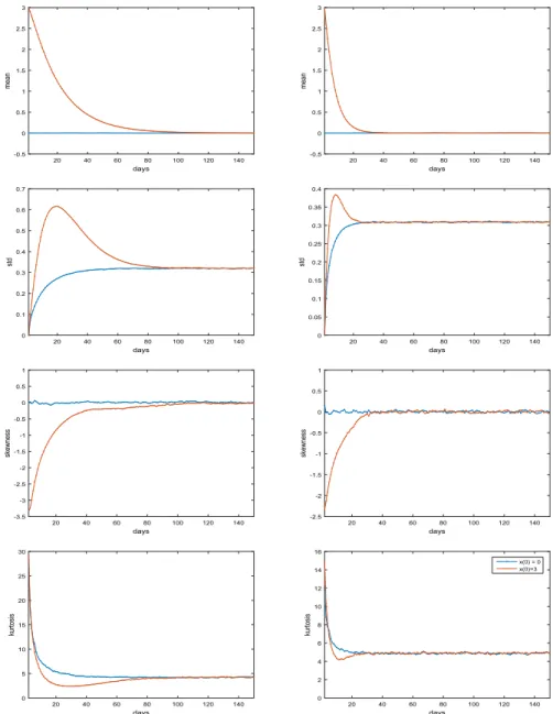
Figure 4 shows the time behavior of the mean, standard deviation, skewness and kurtosis (hereinafter, the first four moments) obtained by Monte Carlo simu-lations using estimated parameters at Palo Verde and PJM markets respectively. Simulations were performed under two very different initial conditions, namely
x(0) = 0 and x(0) = 3 . The first value was chosen equal to the long-run mean value of x(t), the second value was chosen very far from the long-run mean value (it corresponds to an electricity price greater than one thousand dollars). In both cases, standard deviation and kurtosis converge rapidly (in some tens of days) to their stationary values. The mean and the skewness converge rapidly to zero. The convergence is faster in the PJM market because of larger values of the mean reversion parameters. Moreover, random variables x(t) and x(s) ( s ≥ t) become uncorrelated in some tens of days. Figure 5 depicts the time behavior of the cor-relation coefficient in the time interval of [0, 150] days simulated by using Palo Verde and PJM estimated parameters. In each panel, the blue line refers to the ini-tial condition x(0) = 0 , and the red line to the iniini-tial condition x(0) = 3 . The third (yellow) line shows the time behavior of the stationary correlation coefficient. Of course, the stationary autocorrelation function does not depend on the initial condition of the dynamics. Due to higher mean-reversion values, both in the base (18) 𝜌(s, t) = e−𝛼(t−s), days 10 20 30 40 50 60 70 80 90 100 std 0 0.05 0.1 0.15 0.2 0.25 0.3 0.35 0.4 days 10 20 30 40 50 60 70 80 90 100 std 0 0.05 0.1 0.15 0.2 0.25 0.3 0.35 0.4 days 10 20 30 40 50 60 70 80 90 100 kurtosi s 0 3 6 9 12 15 days 10 20 30 40 50 60 70 80 90 100 kurtosi s 0 3 6 9 12 15 Model1 Model 2
Fig. 3 Time behavior of standard deviation and kurtosis simulated using Palo Verde (left panels) and PJM (right panels) estimated parameters
regime and in the turbulent regime, the convergence toward zero correlation is faster for PJM market prices.
The discussed results are very useful to investigate the long-term behavior of electricity prices. Valuing investments in the power sector for new generating capac-ity requires to take into account revenues from selling electriccapac-ity on power market
days 20 40 60 80 100 120 140 mean -0.5 0 0.5 1 1.5 2 2.5 3 days 20 40 60 80 100 120 140 mean -0.5 0 0.5 1 1.5 2 2.5 3 days 20 40 60 80 100 120 140 std 0 0.1 0.2 0.3 0.4 0.5 0.6 0.7 days 20 40 60 80 100 120 140 std 0 0.05 0.1 0.15 0.2 0.25 0.3 0.35 0.4 days 20 40 60 80 100 120 140 skewness -3.5 -3 -2.5 -2 -1.5 -1 -0.5 0 0.5 1 days 20 40 60 80 100 120 140 skewness -2.5 -2 -1.5 -1 -0.5 0 0.5 1 days 20 40 60 80 100 120 140 kurtosis 0 5 10 15 20 25 30 days 20 40 60 80 100 120 140 kurtosi s 0 2 4 6 8 10 12 14 16 x(0) = 0 x(0)=3
Fig. 4 Time behavior of the first four moments simulated using estimated parameters at Palo Verde mar-ket (left panels) and at PJM (right panels). The initial condition is set at x(0) = 0 (blue line) and x(0) = 3 (red line)
for decades. We will see that such results can be used to conciliate accurate descrip-tions of short-term behavior with long-term macroeconomic views about future trends of electricity prices.
4 The stochastic net present value of power generation and the stochastic levelized cost of electricity
The stochastic Net Present Value (NPV) and the stochastic Levelized Cost Of Elec-tricity (LCOE) are mathematical constructs that allow us to introduce risk into the evaluation process of investments in new generating technologies [28, 45]. As speci-fied in the Introduction, we will consider in this paper five sources of risk, namely the risk associated to random movements of (1) electricity prices, (2) gas, (3) coal prices, (4) nuclear fuel and (5) CO2 prices.
To briefly introduce some basic concepts about stochastic NPV and LCOE, let us consider an investment project in a generating plant, financially seen as a cash-flow stream defined on a yearly timetable (as depicted in Fig. 6). We denote by
n = −N <0 the construction starting time, and by n = 0 the end of construction
time. The time n = 0 is also the starting time of the operations, and n = M ≥ 1 is the end of operations time. The cash-flow evaluation time is n = 0.
We suppose that there are k risk sources and we denote by 𝜉 the risky sources stochastic path. The unlevered cash-flow generated by the project at time n, Fz
n , can
be expressed as follows, where Rz
n(𝜉) accounts for stochastic revenues from selling electricity, C z
n(𝜉) for
sto-chastic costs, and Tn(𝜉) for income taxes in the year n. Revenues, costs, and taxes
incurring in the time interval [n − 1, n] are computed as lump sums and valued at time n. All these quantities are expressed in nominal terms. The cost term in Eq. (19) includes all the costs incurred during the whole the operational lifetime of (19) Fnz(𝜉) = Rz n(𝜉) − C z n(𝜉) − T z n(𝜉), n =1, 2, … , M, days 20 40 60 80 100 120 140 corr -0.2 0 0.2 0.4 0.6 0.8 1 days 20 40 60 80 100 120 140 corr 0 0.2 0.4 0.6 0.8 1 x(0) = 0 x(0) = 3 stationary
Fig. 5 Time behavior of the correlation coefficient simulated by using Palo Verde (left panel) and PJM (right panel) estimated parameters
the plant, namely fixed and variable operation and maintenance (O&M) costs, fuel costs (not included in the variable O&M costs), waste management (for nuclear gen-eration) and decommissioning costs. With regard to fossil fuels, costs can include externalities, i.e., environmental costs like CO2 market costs.
In the classic definition, the NPV of an investment in the generating technology z is determined by the difference between the present value of expected revenues and the present values of expected costs and taxes including pre-operations investment costs. NPV can be, then, determined by subtracting investment costs from the pre-sent value of the unlevered cash-flow. To compute the prepre-sent value, the unlevered cash-flow must be discounted at the Weighted Average Cost of Capital (WACC) nominal rate [46]. If we denote by r the nominal WACC rate on an annual basis, the NPV formula reads
In Eq. (20) Iz
0 is the pre-operations nominal investment, starting at n = −N and end-ing at n = 0 , computed as a lump sum, namely as
where ̂Iz
n is the nominal amount of the construction cost allocated to year n.
Follow-ing the MIT [34, 35] analytical approach, yearly tax liabilities are computed by sub-tracting costs and asset depreciation from sales revenues, thus getting
where Dz
n is the fiscal depreciation. Finally, revenues from electricity sales can be
cast as follows,
where Qz is the amount of electricity generated by the technology z in 1 year1, and
Pz
n(𝜉) is the (yearly averaged) unitary selling price of the electricity produced in the
year n by the technology z. By substituting Eq. (19) into Eq. (20) and accounting for Eqs. (22) and (23), after some algebraic manipulations, we get
(20) NPVz= M ∑ n=1 E[Fz n(𝜉) ] (1 + r)n − I z 0. (21) Iz 0= ̂I z −N(1 + r) N + ⋯ + ̂I−1z (1 + r) + ̂I z 0, (22) Tnz(𝜉) = Tc[Rz n(𝜉) − C z n(𝜉) − D z n], (23) Rzn(𝜉) = QzPz n(𝜉),
1 Qz is assumed to be constant over time and can be computed by multiplying the nameplate power capacity of the plant, Wz , by the capacity factor of that plant, CFz , and by the number of hours in 1 year (8760), i.e,
z
= 8760 × CFz × Wz.
where we posed
Equation (24) can be also used as a starting point to determine the Levelized Cost Of Electricity (LCOE) of a given technology.
By definition, the LCOE of the technology z, henceforth denoted by PLC,z , is that deterministic nonnegative real price of the electricity produced by the specific gen-eration technology z, assumed constant over time, that makes the NPV equal to zero. The LCOE is hence a break-even reference unitary cost, i.e., the break-even cost per MWh of produced electricity2. To get the analytical form of PLC,z , let us pose where i is the expected yearly inflation rate and nb labels the base year (which is
used to transform real prices into nominal prices). By substituting Eq. (26) into Eq. (24) and equating NPVz to zero, we obtain
In order to include into the analysis the risk due to random movements of revenues and costs, we must extend the classic NPV metrics. Now we are going to define the
stochastic NPV. Such a definition must satisfy the constraint that the classic NPV
must coincide with the mean of the stochastic NPV, i.e.,
We hence define the stochastic NPV of the technology z as the random variable (24) NPVz= (1 − Tc)Q z M ∑ n=1 E[Pzn(𝜉)]F0,n+ − (1 − Tc) M ∑ n=1 E[Czn(𝜉)]F0,n+ Tc M ∑ n=1 DznF0,n− Iz 0, (25) F0,n= 1 (1 + r)n. (26) E[Pzn(𝜉)] = (1 + i)n−nbPLC,z, (27) PLC,z= ∑M n=1E�C z n(𝜉)�F0,n Qz∑M n=1(1 + i)n−nbF0,n + I z 0− Tc ∑M n=1D z nF0,n (1 − Tc)Qz∑M n=1(1 + i)n−nbF0,n . (28) NPVz= E[NPVz(𝜉)]. (29) NPVz(𝜉) = (1 − Tc)Qz M ∑ n=1 Pzn(𝜉)F0,n − (1 − Tc) M ∑ n=1 Cz n(𝜉)F0,n+ Tc M ∑ n=1 Dz nF0,n− I z 0.
2 LCOE represents the generating costs at the plant level (busbar costs) and does not include
Starting from the definition of the stochastic NPV of the technology z, it is straight-forward to introduce the stochastic LCOE of the technology z. Let us denote by
PLC,z(𝜉) the stochastic LCOE of the technology z. PLC,z(𝜉) is defined path by path as that nonnegative real price of the electricity produced by the specific generation technology z, assumed constant over time, that makes the stochastic NPVz(𝜉) equal
to zero. To get the analytical form of the stochastic LCOE, let us pose thus obtaining from Eq. (29),
As in the case of the stochastic NPV, Eq. (31) shows that the mean of the stochastic LCOE coincides with the classic, deterministic LCOE.
By substituting Eq. (31) into Eq. (29) we can obtain a very useful relationship between the stochastic NPV and the stochastic LCOE of the generation technology z, namely
We remark that the relevant quantity for evaluating an investment in a generating technology is not the NPV itself (for which doubling the size of a plant would dou-ble the NPV), but the unitary NPV, i.e., the NPV per unit of generated electricity. We can, therefore, introduce a ‘reduced stochastic NPV’ in the following form,
The reduced stochastic NPV can be cast in a much more expressive form. From Eq. (32) we namely get
where
Equation (34) clearly shows that break-even or profitability can be reached if and only if E[ ̂Pz(𝜉)]
≥PLC,z (it means that the right quantity to be compared with the
deterministic LCOE is E[ ̂Pz(𝜉)] ). For dispatchable baseload technologies, such as (30) Pzn(𝜉) = (1 + i)n−nbPLC,z(𝜉), (31) PLC,z(𝜉) = ∑M n=1C z n(𝜉)F0,n Qz∑M n=1(1 + i)n−nbF0,n + I z 0− Tc ∑M n=1D z nF0,n (1 − Tc)Qz∑M n=1(1 + i)n−nbF0,n . (32) NPVz(𝜉) = (1 − T c)Qz M ∑ n=1 [Pz n(𝜉) − P LC,z(𝜉)(1 + i)n−nb]F 0,n. (33) NPVz red(𝜉) = NPVz(𝜉) (1 − Tc)Qz ∑M n=1(1 + i) n−nbF 0,n . (34) NPVz red(𝜉) = ̂P z (𝜉) − PLC,z(𝜉), (35) ̂ Pz(𝜉) = ∑M n=1P z n(𝜉)F0,n ∑M n=1(1 + i)n−nbF0,n .
nuclear, coal or combined-cycle gas turbines (CCGTs), which can have the same electricity output profile, Pz
n is a technology independent quantity, i.e.,
where Pb
n denotes the (yearly averaged) unitary selling price of the baseload
genera-tion in the year n. In such a case, Eq. (34) becomes where
Very often in the literature, the classic LCOE is used as a metric to compare gen-eration costs of different technologies [9, 22]. That is, the classic LCOE metric has been used as an alternative to the classic NPV metric. For baseload generation, an economic comparison through LCOE makes sense because, as shown by Eq. (37), the technology that maximizes the expected reduced NPV is the technology that minimizes LCOE. This close link between the LCOE methodology and the financial notion of NPV ‘has always heightened its appeal’ [22]. This simple metric allows for a straightforward comparison of technologies that have different sizes, different life-times and different cost profiles in both regulated and liberalized electricity markets. However, in the case of Variable Renewable Energy (VRE) sources, such as wind or solar sources, ̂Pz
n(𝜉) can be a technology dependent parameter. Namely, in liberalized
markets the hourly electricity output profile of non-dispatchable technologies can significantly differ between each other, and the LCOE evaluation approach should be carefully used for comparative purposes. Well aware of this, some Authors tried to investigate timing impact of electricity generation from VRE sources [23, 43]. In any case, being the LCOE a break-even reference unitary cost, it is a useful refer-ence cost metric which can be compared with expected electricity market prices for checking, on the basis of Eq. (34), if break-even can be reached.
The next sections will be devoted to compute stochastic revenues and costs. Our aim ere his to provide a model to evaluate long-run investments in new generation technologies under uncertainty through the stochastic NPV metric. Without loss of generality, in the following we assume that the evaluation time, n = 0 , coincides with the base year, nb.
5 Modeling revenues
When modeling revenues, we assumed that the dynamics of electricity prices is described by Model 3, the more realistic model that well reproduces most of the observed features of market prices. This model was calibrated on past data, in a backward looking way, separating the deterministic component of Eq. (2) from the (36) Pzn(𝜉) = Pb n(𝜉), (37) NPVz red(𝜉) = ̂P b(𝜉) − PLC,z(𝜉), (38) ̂ Pb(𝜉) = ∑M n=1P b n(𝜉)F0,n ∑M n=1(1 + i)n−nbF0,n .
stochastic component. Since we now want to include macroeconomic forward look-ing information, we can replace in Eq. (2) the values of b0 and b1 related to the linear (affine) trend with new values that can account for macroeconomic views on the future long-term evolution of electricity prices. The 𝛽0 and 𝛽1 parameters will be determined in a such a way to match the expected long-run mean, the expected infla-tion rate, and the expected real escalainfla-tion rate of power prices. Such macroeconomic estimates can be found in the Annual Energy Outlook 2019 [9] provided by the US Energy Information Administration.
According to both classic and stochastic NPV approaches the revenues from sell-ing electricity dursell-ing the annual time interval [n − 1, n] must be computed as a lump sum valued at time n. Limiting our analysis to baseload generation, the revenues term of Eq. (37) can be computed assuming that Pb
n is the annual averages of daily
market prices, i.e.,
where 𝛽0 and 𝛽1 account for a forward looking linear (affine) trend. Such parameters go to replace b0 and b1 . P0(tkn) denotes the electricity price at the kth day of the nth
year, computed with b0= b1= 0 . The dependence on the path 𝜉 will be henceforth omitted. To investigate the statistical properties of Pb
n , let us consider the detrended
log-revenues process, hb
n , given by
Figure 7 shows the time behavior of the 1-year autocorrelation of hb
n as n varies on
a 30-year time horizon, computed using estimated parameters at Palo Verde and PJM markets. Figure 8 depicts the time behavior of the first four moments of the detrended log-revenues process as as n varies on a 30-year time horizon.
We notice that the random variables hb
n ( n ≥ 1 ) are uncorrelated random variables
with same mean, ̄hb (about 0.06 at Palo Verde, and 0.05 at PJM), same standard deviation, 𝛴b (about 9.46% at Palo Verde, and 5.37% at PJM), zero skewness and kurtosis equal to three. Moreover, we performed some tests of normality, such as the Jarque-Bera test, the Kolmogorov-Smirnov test, the Anderson-Darling test and (39) Pbn= e𝛽0+𝛽1n [ 1 365 365 ∑ k=1 P0(tkn) ] , (40) hbn= log Pbn− 𝛽0− 𝛽1n.
Fig. 7 One-year autocorrelation of the detrended log-revenues process years 0 5 10 15 20 25 30 one-year cor r -0.3 -0.2 -0.1 0 0.1 0.2 0.3
the chi-square test on Monte Carlo generated samples with sample size of five thou-sands trials. All these tests reveal that the hypothesis of normality for hb
n ( n ≥ 1 )
can-not be rejected. As a consequence, we assume that hb
n ( n ≥ 1 ) are i.i.d. normal
ran-dom variable with mean ̄hb and standard deviation 𝛴
b , i.e., hbn∼ N( ̄hb, 𝛴
2
b) . This is an important result which is very useful to compute revenues from selling electricity on a long-term timescale.
Now we need to determine 𝛽0 and 𝛽1 . This can be done using macroeconomic views about the long-run behavior of power prices. We thus require that
where Ab is the current annual average of the electricity generation price, and where 𝜋 = ln(1 + i) and 𝜋b accounts for the view on the real escalation rate of power prices, i.e., 𝜋b= ln(1 + kb) with kb the expected real escalation rate of power prices. The Annual Energy Outlook 2019 [9] provides the following values, Ab= 64 $
2018 per MWh, i = 2.3% per annum, and kb= −0.5% per annum.
Finally, we point out that the above analysis could also have been carried out using Model 1 or Model 2, which are special cases of Model 3. However, the esti-mate of the log-revenues standard deviation parameter, 𝛴b , could be affected by errors due to a naive choice of the short-term model. In fact, Model 1 underesti-mates the log-revenues standard deviation (about 6.16% at Palo Verde, and 4.79% at
(41) exp(𝛽0+ ̄hb+ 1 2𝛴 2 b) = A b, (42) 𝛽1= 𝜋 + 𝜋b, years 0 5 10 15 20 25 30 mean 0 0.01 0.02 0.03 0.04 0.05 0.06 0.07 0.08 0.09 0.1 years 0 5 10 15 20 25 30 std 0 0.05 0.1 0.15 years 0 5 10 15 20 25 30 skewness -1 -0.8 -0.6 -0.4 -0.2 0 0.2 0.4 0.6 0.8 1 years 0 5 10 15 20 25 30 kurtosi s 2 2.2 2.4 2.6 2.8 3 3.2 3.4 3.6 3.8 4 Palo Verde PJM
PJM) and, on the contrary, Model 2 overestimates such a parameter (about 10.93% at Palo Verde, and 5.94% at PJM). Although these values differ slightly in the case of PJM, such differences become large in the case of Palo Verde, especially for Model 1. This fact has important consequences on the shape of the probabilistic distribu-tion of the stochastic NPV leading to an incorrect assessment of the risk associated with the investment [28]. This would lead energy companies and policy makers to misjudge the risk associated with new investments in power generation. For these reasons, in the empirical analysis discussed in Sect. 7 we will use the standard devi-ation value estimated on Palo Verde market data using Model 3.
6 Modeling fuel price dynamics
To compute stochastic NPVs of new generating technologies we need to determine the stochastic behavior of fuel costs. In this section, we accurately model the sto-chastic dynamics of fuels and CO2 prices which are the main sources of risk when power generating costs are considered.
6.1 Modeling fossil fuel prices
Figure 9 shows the historical behavior of natural gas and coal prices. Our data set consists of time series of gas and coal prices at a monthly frequency since January, 1999 until November, 2018. Prices are expressed in nominal dollars per mmBtu, i.e., nominal dollars per million Btus. Data refer to the cost of natural gas and coal receipts at electric generating plants, and they were downloaded from the US Energy Information Administration at site www.eia.doe.gov/total energ y/data.
Figure 10 shows the historical behavior of fossil fuel log-returns, calculated as monthly changes in the natural logarithm of monthly prices. Table 7 displays the descriptive statistics of fossil fuel log-returns.
The empirical analysis reveals that the time series of gas and coal log-returns do not show infra-annual seasonality and are almost uncorrelated (the correlation coef-ficient in the period under investigation is about − 0.0052).
19992 2006 2012 2018 4 6 8 10 12 14 monthly price s Natural gas 1999 2006 2012 2018 monthly prices 1 1.5 2 2.5 Coal
Fig. 9 Historical behavior of fossil fuel market prices since January, 1999–November, 2018. Left panel: natural gas. Right panel: coal
Geometric Brownian Motion (GBM) is often used in the literature to model fossil fuel price dynamics [21, 33]. However, looking at Fig. 10, it seems that such process cannot be able to fully capture the observed dynamics of gas log-returns. Evidence exists for a more complicated behavior of gas prices showing mean-reversion, jumps and stochastic volatility [15]. We propose, therefore, a stochastic model, in which the time evolution of of gas prices is described by a mean-reverting jump-diffusion model. In contrast, to describe the dynamics of coal prices we use a GBM stochastic process. Observed coal prices, in fact, do not show mean-reversion patterns in the period under investigation, and the kurtosis value (3.3687) is consistent with nor-mally distributed log-returns.
6.1.1 Modeling natural gas price dynamics
To model the gas price dynamics, let us denote by Pga(t) the gas market price at time
t (the suffix ‘ga’ stands for ‘gas’), expressed in nominal dollars per mmBtu, and by sga(t) = ln Pga(t) its natural logarithm. We assume that sga(t) can be decomposed as follows,
where bga
0 accounts for a constant trend and xga(t) for the stochastic component of the dynamics. In the period under investigation, the gas price dynamics does not show any linear trend and the empirical analysis confirms this feature. We estimated
bga0 on market data using Ordinary Least Squares (OLS) techniques, thus finding bga0 = 1.5224 . Looking at the left panel of Fig. 9, it is worth to observe that US natu-ral gas market went through important transitions in the sample period. In the early 2000s, prices were trending upward as conventional US natural gas production was (43) sga(t) = bga 0 + x ga(t), 1999 2006 2012 2018 -0.4 -0.3 -0.2 -0.1 0 0.1 0.2 0.3 0.4 0.5 monthly log-return s Natural gas 1999 2006 2012 2018 -0.1 -0.08 -0.06 -0.04 -0.02 0 0.02 0.04 0.06 0.08 0.1 monthly log-return s Coal
Fig. 10 Historical behavior of fossil fuel log-returns since January, 1999–November, 2018. Left panel: natural gas. Right panel: coal
Table 7 Descriptive statistics of
fossil fuel log-returns Mean St. dev. Skewness Kurtosis
Gas 0.0026 0.1091 0.3132 4.6335
declining over time, then the boom in unconventional gas production coincided with a persistent decrease in natural gas prices in the 2010s. Moreover, gas prices were trending upward again at the end of 2010s and macroeconomic projections to 2050 show a persistent upward trend in prices [9]. Over very long time horizons such trend changes can be considered as random events and we account for them in the stochastic component of the dynamics through a mean-reversion mechanism in a jump-diffusion process. We assume, therefore, that the time evolution of the sto-chastic component of the gas price dynamics, xga(t) , is described by the following stochastic differential equation,
where wga(t) is a Wiener process and qga(t) is a Poisson process with constant inten-sity 𝜆ga . The random jump amplitude Jga is distributed according to a normal ran-dom variable with zero mean and standard deviation 𝜎ga
J , i.e., J ∼ N(0, (𝜎
ga
J )2
) . We assume that the Wiener process wga , the Poisson process qga , and the jump amplitude
Jga are mutually independent processes. The stochastic component of the dynamics was estimated on market data by maximum likelihood using the Euler discretization with time step 𝛥t equal to 1 month. Estimation results are depicted in Table 8.
The statistical analysis of simulated trajectories confirms that the jump-diffusion model offers an interesting agreement with market data. The first four moments of paths log-returns, obtained averaging over ten thousands paths randomly generated using estimated parameters, are displayed in Table 9.
In computing the stochastic NPV of gas generation, gas costs incurred in the annual time interval [n − 1, n] must be computed as a lump sum and valued at time
n. We assume that such costs (per mmBtu) in the year n are determined as a monthly
market price average, Pga
n , given by (44) dxga(t) = −𝛼gaxga(t)dt + 𝜎gadwga(t) + Jgadqga(t), (45) Pgan = e𝛽0ga+𝛽1gan[ 1 12 12 ∑ k=1 Pga(tkn) ] ,
Table 8 Estimation results of the stochastic component of the gas price dynamics
Standard errors are between parentheses
𝛼ga 𝜎ga 𝜆ga 𝜎ga
J
0.0408 0.0789 0.2532 0.1447
(0.0095) (0.0083) (0.0426) (0.0159)
Table 9 Statistics of simulated paths log-returns using estimated parameters
Standard deviations are between parentheses
Mean St. dev. Skewness Kurtosis
0.0030 0.1086 0.0033 4.6346
where 𝛽ga 0 and 𝛽
ga
1 account for a forward looking linear (affine) trend, and tkn denotes
the kth month of the nth year. The dependence on the path 𝜉 has been omitted. The parameters 𝛽ga
0 and 𝛽 ga
1 allow us to calibrate the model on macroeconomic views about the future trend of gas market prices.
To investigate the statistical properties of Pga
n , let us consider the detrended log-cost
process given by
Figure 11 shows the time behavior of the autocorrelation function (left panel) and the 1-year autocorrelation (right panel) of hga
n ( n ≥ 1 ) as n varies on a 30-year time
(46) hgan = log Pga n − 𝛽 ga 0 − 𝛽 ga 1 n. years 5 10 15 20 25 30 corr -0.2 0 0.2 0.4 0.6 0.8 1 years 0 5 10 15 20 25 30 one-year corr 0 0.1 0.2 0.3 0.4 0.5 0.6 0.7 0.8 0.9 1
Fig. 11 The autocorrelation function of the detrended log-cost process (left panel), and the 1-year auto-correlation function (right panel)
year 0 5 10 15 20 25 30 mean -0.1 -0.08 -0.06 -0.04 -0.02 0 0.02 0.04 0.06 0.08 0.1 years 0 5 10 15 20 25 30 std 0 0.05 0.1 0.15 0.2 0.25 0.3 0.35 0.4 0.45 0.5 years 0 5 10 15 20 25 30 skewness -1 -0.8 -0.6 -0.4 -0.2 0 0.2 0.4 0.6 0.8 1 years 0 5 10 15 20 25 30 kurtosi s 2 2.2 2.4 2.6 2.8 3 3.2 3.4 3.6 3.8 4
horizon, computed with estimated parameters. Figure 12 depicts the time behavior of the first four moments of hga
n as n varies on a 30-year time horizon, computed with
estimated parameters. We noticed that the random variables hga
n ( n ≥ 1 ) are
corre-lated random variables with a constant correlation coefficient, which is approxi-mately equal to 0.7. After a transient period of about 3 year, such random variables are characterized by the same values of mean, ̄hga (about 0.02), and the same value of the standard deviation, 𝛴ga (about 0.35), zero skewness and kurtosis equal to three. Moreover, we performed some tests of normality such as the Jarque–Bera test, the Kolmogorov–Smirnov test, the Anderson–Darling test and the chi-square test on Monte Carlo generated samples with sample size of five thousands trials. All these tests reveal that the hypothesis of normality for hb
n ( n ≥ 1 ) cannot be rejected. We
assume, therefore, that hga
n ( n ≥ 1 ) are correlated i.d. normal random variable with
mean ̄hga and standard deviation 𝛴
ga , i.e., h ga
n ∼ N( ̄hga, 𝛴ga2) . This is a further
impor-tant result, useful to compute gas costs on a long-term horizon.
The calibration of the model on macroeconomic views about long-term behavior of gas prices can proceed as in the electricity case. Namely, we require that
where Aga is the current annual average of the gas price, and
where 𝜋ga accounts for the view on the real escalation rate of gas prices, i.e.,
𝜋ga= ln(1 + kga) and kga is the expected real escalation rate of gas prices. The Annual Energy Outlook 2019 [9] provides the following values, Aga= 3.54 $
2018 per mmBtu, and kga= 1.4% per annum. Such values are also reported in Table 10.
6.1.2 Modeling coal price dynamics
To model the coal price dynamics, let us denote by Pco(t) the coal market price at time t (the suffix ‘co’ stands for ‘coal’), expressed in nominal dollars per mmBtu. We assume that the dynamics of Pco(t) is described by a GBM process of the type,
where wco(t) is a Wiener process. The volatility parameter is set at the value 0.0143 on a monthly basis (see Table 7), i.e., 𝜎co= 0.05 on an annual basis. The drift coef-ficient accounts for the expected inflation, 𝜋 , and the expected real escalation rate of coal prices, 𝜋co= ln(1 + kco) , where kco is the expected real escalation rate of coal prices. The Annual Energy Outlook 2019 [9] provides the value kco= 0.2% per annum. Such value is also reported in Table 10. Since the correlation between coal market prices and power market prices is negligible [21], the Wiener process, wco(t) , is assumed to be independent from the stochastic processes driving the time evo-lution of power prices and gas prices. Differently from mean-reverting processes,
(47) exp(𝛽ga 0 + ̄h ga+ 1 2𝛴 2 ga) = A ga, (48) 𝛽ga 1 = 𝜋 + 𝜋 ga, (49) dPco(t) Pco(t) = (𝜋 co+ 𝜋)dt + 𝜎codwco(t),
Geometric Brownian Motion has not stationary solutions for the probability density function. Then, the coal cost evaluation in computing the stochastic NPV of coal plants is performed pointwise at the end of each year using Equation (49) with an initial condition given by the coal price value reported in Table 10.
6.2 Modeling nuclear fuel prices
Our data set consists of a time series of nuclear fuel prices at an annual frequency since 1973 until 2017. Data can be downloaded from the US Energy Information Administration at site www.eia.doe.gov/opend ata. Figure 13 shows the historical behavior of nuclear fuel prices (left panel) and their annual log-returns, calculated as annual changes in the natural logarithm of prices (right panel). Prices are expressed in nominal dollars per mmBtu.
1978 1988 1998 2008 2018 annual prices 0.1 0.2 0.3 0.4 0.5 0.6 0.7 0.8 Nuclear fuel 1978 1988 1998 2008 2018 annual log-return s -0.1 -0.05 0 0.05 0.1 0.15 0.2 0.25 Nuclear fuel
Fig. 13 Historical behavior of nuclear fuel prices (left panel) and log-returns (right panel) since 1973– 2017
Table 10 Technical assumptions
‘mill’ stands for 1/1000. Depreciation is developed according to the MACRS (Modified Accelerated Cost Recovery System) scheme
Units Gas Coal Nuclear
Nominal capacity factor 87% 85% 90%
Heat rate Btu/kWh 6600 8800 10461
Overnight cost $/kW 999 3747 6034
Fixed O&M costs $/kW/year 11.33 43.37 103.31
Variable O&M costs mill $/kWh 3.61 4.74 2.37
Fuel costs $/mmBtu 3.54 2.11 0.75
Fuel real escalation rate 1.4% 0.2% 0.2%
Decommissioning $/kW 50 200 1000
CO2 intensity Kg-C/mmBtu 14.5 25.5 0
Construction period # of years 3 4 6
Plant life # of years 30-40 30-40 30-40-60
Let us denote by Pnu(t) the nuclear fuel price at time t (the suffix ‘nu’ stands for ‘nuclear’). In the period under investigation log-returns do not show mean-rever-sion, and we assume that the dynamics of nuclear fuel prices is described by a GBM process of the type
where wnu(t) is a Wiener process and 𝜋nu= ln(1 + knu) , being knu the expected real escalation rate of nuclear fuel prices. The Annual Energy Outlook 2019 [9] provides the following value knu= 0.2% per annum, as reported in Table 10. The Wiener pro-cess, wnu(t) , is assumed to be independent from the stochastic processes driving the time evolution of power prices and fossil fuel prices.
The volatility parameter was estimated by maximum likelihood on the nuclear fuel dataset. We obtained the value 𝜎nu= 0.07 on an annual basis. As in the coal case, the nuclear fuel cost evaluation for computing the stochastic NPV of nuclear power plants is performed pointwise at the end of each year using Eq. (50) with an initial condition given by the nuclear fuel price value reported in Table 10.
6.3 Modeling CO2 prices
Let us denote by Pca(t) the CO
2 price at time t (the suffix ‘ca’ stands for ‘carbon’), expressed in nominal dollars per ton of CO2 . The dynamics of CO2 prices, is mod-eled according to a GBM process of the type
where 𝜎ca is the carbon volatility and wca(t) is a Wiener process which is assumed to be independent from the stochastic processes driving the time evolution of power prices, fossil fuel prices, and nuclear fuel prices. However, the model can be extended to account for a possible correlation between CO2 prices and power prices. A CO2 price equal to 30 $2018 per ton of CO2 [7, 22] is assumed as initial condition of the CO2 price process. Regarding the volatility, we consider a CO2 price volatility
𝜎ca= 20% . These assumptions try to depict a realistic scenario in order to inves-tigate the impact of CO2 volatility on the risk of investments in fossil fuel power plants [14]. The contribution of CO2 costs to the stochastic NPV is computed point-wise at the end of each year.
7 The stochastic NPV of generating electricity
Table 10 details technical data and costs used in the empirical analysis. The main data source is the ‘Annual Energy Outlook 2019’ [9]. In particular, the cost of new generating technologies are taken from ‘Capital Cost Estimates for Utility Scale Electricity Generating Plants’ [12] and ‘Cost and Performance Character-istics of New Generating Technologies, Annual Energy Outlook 2019-January
(50) dPnu(t) Pnu(t) = (𝜋 nu+ 𝜋)dt + 𝜎nudwnu(t), (51) dPca(t) Pca(t) = 𝜋dt + 𝜎 cadwca(t),
2019’ [10], both provided by the US Energy Information Administration. Data refer to a Conventional Natural Gas Combined Cycle (NGCC) facility for the gas technology, to an Ultra Supercritical Coal (USC) facility for the coal technology, and to an advanced PWR (Pressurized Water Reactor) nuclear power facility. All costs are denominated in year 2018 US dollars ( $2018 ). With the exception of the nuclear technology, decommissioning costs were set at about 5% of the overnight cost [22, 42]. For nuclear power plants we assumed a larger percentage of the overnight cost to account for decommissioning and radioactive waste disposal [39, 51]. Overnight costs are uniformly distributed on the construction period. In accordance to the Annual Energy Outlook 2019 (AEO 2019), we assumed an expected inflation rate i = 2.3% per annum, and a corporate tax rate Tc= 21% as
specified in the Tax Cuts and Jobs Act of 2017. As in AEO 2019, all LCOE cal-culations are performed using a nominal after-tax WACC rate of 7.0% per annum [9, 11].
Probabilistic distributions of stochastic LCOE and reduced NPV [equation (hereinafter NPV)] of new generating technologies can be obtained by using Monte Carlo techniques. Random paths for electricity prices, fuel prices, and CO2 prices are generated according to dynamic models illustrated in the previous sec-tion. Along such paths, LCOE and NPV values are computed by using LCOE and NPV formulas reported in Sect. 4. Numerical computations are performed without and with CO2 stochastic costs. In this last case, we assumed that macro-economic views on the future evolution of power prices as well as their volatility are not influenced by the inclusion of carbon costs. Computations are performed under the hypothesis of zero correlation between (unitary) revenues and costs. This is not a strong assumption, even in the case of gas fired plants. The empirical analysis developed in the previous sections revealed that annual revenues are not correlated over time. On the other side, gas generation annual costs show a high positive correlation over time. This implies that, although gas and power prices could show some cointegration relationship [36], nevertheless the correlation between annual revenues and costs, if there is any, must be negligible. However, the model can be extended in a straightforward way to include such a correlation.
Figure 14 depicts simulated distributions of the stochastic LCOE (without and with CO2 costs) of baseload sources computed on a 30-year plant lifetime.
20 30 40 50 60 70 80 90 100 0 0.05 0.1 0.15 0.2 0.25 0.3 20 40 60 80 100 120 140 0 0.05 0.1 0.15 0.2 0.25 0.3 Gas Coal Nuclear
Fig. 14 Stochastic LCOE distributions without CO2 costs (left panel) and with CO2 costs (right panel)