Dottorato di Ricerca in FISICA
Ciclo XXII
Coordinatore: Prof. Filippo Frontera
Management, Optimization and
Evolution of the LHCb Online
Network
Candidato: Guoming Liu
Tutore: Prof. Mauro Savri`e
Co-Tutore: Dr. Niko Neufeld (CERN)
The LHCb experiment is one of the four large particle detectors running at the Large Hadron Collider (LHC) at CERN. It is a forward single-arm spectrom-eter dedicated to test the Standard Model through precision measurements of Charge-Parity (CP) violation and rare decays in the b quark sector. The LHCb experiment will operate at a luminosity of 2 × 1032cm−2s−1, the proton-proton
bunch crossings rate will be approximately 10 MHz. To select the interesting events, a two-level trigger scheme is applied: the first level trigger (L0) and the high level trigger (HLT). The L0 trigger is implemented in custom hardware, while HLT is implemented in software runs on the CPUs of the Event Filter Farm (EFF). The L0 trigger rate is defined at about 1 MHz, and the event size for each event is about 35 kByte. It is a serious challenge to handle the resulting data rate (35 GByte/s).
The Online system is a key part of the LHCb experiment, providing all the IT services. It consists of three major components: the Data Acquisition (DAQ) system, the Timing and Fast Control (TFC) system and the Experiment Control System (ECS). To provide the services, two large dedicated networks based on Gigabit Ethernet are deployed: one for DAQ and another one for ECS, which are referred to Online network in general. A large network needs sophisticated moni-toring for its successful operation. Commercial network management systems are quite expensive and difficult to integrate into the LHCb ECS. A custom network monitoring system has been implemented based on a Supervisory Control And Data Acquisition (SCADA) system called PVSS which is used by LHCb ECS. It is a homogeneous part of the LHCb ECS. In this thesis, it is demonstrated how a large scale network can be monitored and managed using tools originally made for industrial supervisory control.
then describes all sub-detectors and the trigger and DAQ system of LHCb from structure to performance.
Chapter 2 first introduces the LHCb Online system and the dataflow, then focuses on the Online network design and its optimization.
In Chapter 3 , the SCADA system PVSS is introduced briefly, then the architecture and implementation of the network monitoring system are described in detail, including the front-end processes, the data communication and the supervisory layer.
Chapter 4 first discusses the packet sampling theory and one of the packet sampling mechanisms: sFlow, then demonstrates the applications of sFlow for the network trouble-shooting, the traffic monitoring and the anomaly detection.
In Chapter 5 , the upgrade of LHC and LHCb is introduced, the possible architecture of DAQ is discussed, and two candidate internetworking technolo-gies (high speed Ethernet and InfiniBand) are compared in different aspects for DAQ. Three schemes based on 10 Gigabit Ethernet are presented and studied.
L’esperimento LHCb, `e uno dei Quattro grandi rivelatori di particelle operanti sul Large Hadron Collider (LHC) del CERN. Esso consiste in uno spettrometro in avanti a braccio singolo, dedicato a misure di precisione della violazione della parit`a/Coniugazione di Carica (CP) finalizzate a sondare la validit`a del modello Standard (SM). L’esperimento LHCb lavorer`a con una luminosit`a nominate L=2∗ 1032cm−2s−1 e una frequenza di bunch crossing (BC) protone protone pari a 10 MHz. La selezione degli eventi `e realizzata mediante un trigger a due livelli: il primo livello (L0) e quello di alto livello (HLT). Il livello L0 `e realizzato mediante elettronica dedicata, mentre lo HLT `e essenzialmente un trigger “software” che opera sulle CPU del complesso di computer dell’EFF (“Event Filter Farm”). La frequenza del primo livello `e circa 1 MHz e la dimensione tipica dell’evento `e di circa 35 Kbytes. La frequenza di dati che ne deriva `e 35 Gbytes/s e costituisce una importante sfida tecnologica.
Il sistema Online `e una parte chiave cruciale dell’esperimento LHCb poich fornisce tutti i servizi informatici (IT). L’infrastruttura `e composta da tre com-ponenti: “Data Acquisition” (DAQ), “Timing and Fast Control” (TFC) and “Experiment Control System” (ECS). Il sistema Online `e stato sviluppato sulla base di due grandi reti dedicate basate su tecnologia Gigabit Ethernet: la “DAQ network” e la “ECS network” che compongono la “Online network”. Reti cos grandi richiedono un costante e affidabile monitoraggio per il corretto funziona-mento e va considerato che sistemi di gestione commerciali sono particolarmente costosi e difficili da integrare in LHCb ECS. Il sistema di monitoraggio di rete che fa parte dell’ECS di LHCb `e stato implementato sulla base di un sistema SCADA (controllo di supervisione e acquisizione dati) chiamato “PVSS”. Questo sistema `e di tipo omogeneo. In questa tesi viene dimostrato come reti di grandi
La tesi `e divisa nel modo seguenete:
Il capitolo 1 contiene una breve introduzione a LHC, alla fisica del quark b e comprende una descrizione di tutti i rivelatori, dei “trigger” e del sistema DAQ di LHCb dal punto di vista dell’infrastruttura e delle prestazioni.
Il capitolo 2 inizialmente introduce il sistema Online di LHCb e descrive il flusso di trasmissione delle informazioni, soffermandosi successivamente sulla pro-gettazione e ottimizzazione della rete.
Nel capitolo 3 viene introdotto PVSS e vengono descritti in dettaglio l’imple-mentazione del sistema di monitoraggio di rete, l’architettura e i suoi componenti: front-end, comunicazioni di dati e “supervisory layer” (strato di supervisione)
Il capitolo 4 inizialmente introduce la teoria del packet sampling e il sistema sFlow adottato. Successivamente si sofferma sull’implementazione di quest’ultimo per il troubleshooting di reti, il monitoraggio del traffico e il rilevamento delle anomalie.
Nel capitolo 5 viene introdotta la programmazione dell’aggiornamento di LHC e di LHCb. Una possibile architettura di rete per la DAQ viene successivamente presentata insieme alle due possibili soluzioni tecnologiche necessarie alla sua implementazione (Ethernet e InfiniBand). Tre proposte di soluzione basate su tecnologia 10G Ethernet vengono presentate e studiate.
I am so grateful for all the support I have received whilst researching and writing up this thesis.
First, I would like to thank Dr. Niko Neufeld, my friend and supervisor at CERN. He lead me into the field of networking and network-based DAQ for high energy physics experiments, he guided and accompanied me at almost every step to this work in a friendly and encouraging way. He always covered me even when I made some stupid mistakes. My work would have been impossible without the great help from Niko. He spent a lot of time to discuss and correct my thesis even during nights and weekends.
Then I would like to express my great gratitude to Prof. Mauro Savri`e, my supervisor in Ferrara University. We spent a lot of time together at my early stage of study, working on Multi-Wire Proportional Chamber (MWPC) for the LHCb Muon detector. Even though this is not directly related to my thesis, I learned from him a lot of knowledge on particle detectors and the methods to do research more importantly. He always supported me throughout my study and encouraged me to develop new interests, he gave me the opportunity to come and work on my thesis at CERN.
I am very grateful to all my colleagues in the LHCb Online Group. As the leader of the Online group, Beat Jost always shown his support and advised me with his great experiences, he also took a lot of my hard work. My friends and colleagues Loic Brarda, Gary Moine, Jean-Christophe Garnier, Enrico Bonaccorsi, Rainer Schwemmer, Juan Manuel Caicedo Carvajal and Alexander Mazurov, they taught me a lot in their areas of expertise, and we had a good collaboration. Clara Gaspar, Alba Sambade Varela and Maria Del Carmen Barandela Pazos gave me a lot of helps and support on PVSS.
not only to my work but also to my life in Ferrara.
A special thanks goes to Prof. Yigang Xie, Prof. Cuishan Gao and Prof. Xiaoxi Xie from Institute of High Energy Physics, China. They introduced me into the field of high energy physics and gave me many useful and constructive advices.
I would also like to thank Carles Kishimoto from CERN IT-CS department and Marc Bruyere from Force10Networks, who gave me a lot of helps on the network devices.
A warm “thank you” goes to all my dear friends who support me all the time. Last but not least I would like to thank my family for their support and encouragement in every single day of my life.
Abstract i
Acknowledgements v
Contents vii
List of Figures xiii
List of Tables xvii
Abbreviations xix
1 The LHCb Experiment 1
1.1 The Large Hadron Collider . . . 1
1.1.1 The Large Hadron Collider Machine . . . 1
1.1.2 The LHC Experiments . . . 3
1.2 The B Physics at LHC . . . 5
1.2.1 Theory Overview: CP Violation in the Standard Model . . 5
1.2.2 B Meson Production at LHC . . . 6
1.3 The LHCb Experiment . . . 8
1.3.1 The Magnet . . . 9
1.3.2 The Vertex Locator . . . 10
1.3.3 Tracking . . . 13
1.3.3.1 Trigger Tracker . . . 13
1.3.3.2 Inner Tracker . . . 14
1.3.4 Particle Identification . . . 17
1.3.4.1 The RICH . . . 18
1.3.4.2 The Calorimeter System . . . 19
1.3.4.3 The Muon Detector . . . 21
1.3.5 The LHCb Trigger and DAQ . . . 23
1.3.5.1 The L0 Trigger . . . 24
1.3.5.2 The High-Level Trigger . . . 26
1.3.5.3 Data Acquisition . . . 26
1.4 Summary . . . 27
2 The LHCb Online System and Its Networks 29 2.1 Data Acquisition . . . 30
2.1.1 Physics Requirements . . . 30
2.1.2 Data Readout . . . 31
2.1.3 High Level Trigger and Data Storage . . . 33
2.2 The Experiment Control System . . . 34
2.3 LHCb Online Networks . . . 36
2.3.1 Control Network . . . 37
2.3.1.1 Architecture of the Control Network . . . 38
2.3.1.2 Interfaces to CERN Network: GPN, TN and LCG 39 2.3.1.3 Redundancy for Critical Services . . . 40
2.3.1.4 Management Network . . . 42
2.3.2 DAQ Network . . . 42
2.3.2.1 Constraints, requirements and choice of technology 42 2.3.2.2 Architecture and Implementation of the DAQ Net-work . . . 44
2.3.2.3 Configuration and Performance of Link Aggregation 46 2.4 Summary . . . 48
3 Network Monitoring with a SCADA System 51 3.1 Introduction to SCADA, PVSS and JCOP . . . 52
3.1.1 Supervisory Control And Data Acquisition (SCADA) . . . 52
3.1.2 PVSS . . . 53
3.2 Architecture of the network monitoring system . . . 56
3.2.1 Data communication: DIM . . . 58
3.2.2 Front-end data collectors . . . 59
3.2.2.1 SNMP collector . . . 59 3.2.2.2 sFlow . . . 62 3.2.3 Supervision layer in PVSS . . . 64 3.2.3.1 Data modeling . . . 64 3.2.3.2 Data processing . . . 67 3.2.3.3 User interfaces . . . 68
3.3 Modules of the network monitoring system . . . 69
3.3.1 Topology discovery and monitoring . . . 69
3.3.1.1 Data sources . . . 71
3.3.1.2 Discovery of switches . . . 72
3.3.1.3 Discovery of end-nodes . . . 73
3.3.1.4 Topology monitoring . . . 76
3.3.2 Network traffic monitoring . . . 77
3.3.3 Network device status monitoring . . . 81
3.3.4 Monitoring of data path for DAQ and interfaces to external network . . . 81
3.3.5 Syslog message monitoring . . . 83
3.3.6 FSM for network monitoring: the user point of view . . . . 85
3.4 Summary . . . 87
4 Advanced Network Monitoring Based on sFlow 89 4.1 Packet Sampling and sFlow . . . 90
4.2 Network debug tool based on sFlow . . . 94
4.3 DAQ monitoring using sFlow . . . 96
4.4 Monitor security threats and anomalies using sFlow and snort . . 98
4.4.1 Introduction to Snort . . . 100
4.4.2 IDS based on sFlow and Snort . . . 102
4.4.3 Discussions on the accuracy of anomaly detection . . . 103
5 Evolution of the LHCb DAQ Network 107
5.1 LHC upgrade . . . 107
5.2 LHCb upgrade . . . 108
5.2.1 The LHCb trigger upgrade . . . 109
5.2.2 Architecture of trigger free DAQ system . . . 109
5.3 High speed networking technology . . . 111
5.3.1 10/40/100 Gb/s Ethernet . . . 112
5.3.2 InfiniBand . . . 114
5.3.3 Comparison of 10/40/100 GbE and InfiniBand . . . 116
5.3.3.1 Performance . . . 116 5.3.3.2 Market . . . 118 5.3.3.3 Difficulty of implementing . . . 119 5.3.3.4 Maturity . . . 119 5.3.3.5 Quality of Service . . . 119 5.3.3.6 Conclusion . . . 121
5.4 Solution of the DAQ network . . . 122
5.4.1 Solution based on high-end switches . . . 122
5.4.2 Solution based on commodity pizza-box switches . . . 123
5.4.3 Solution based on merchant networking ASIC . . . 125
5.4.4 Conclusion . . . 126
5.5 Study of the solution based on commodity pizza-box switches . . 127
5.5.1 Network simulation . . . 127
5.5.1.1 Simulation results of the scheme without opti-mization . . . 128
5.5.1.2 Simulation results of the scheme with optimization 129 5.5.1.3 The rate of packet drop . . . 130
5.5.2 Network management . . . 131
5.6 Summary . . . 133
6 Conclusions 135
B Switching Methods 139 B.1 Store-and-forward switching . . . 139 B.2 Cut-through switching . . . 140 B.3 Fragment-free switching . . . 140
1.1 Basic layout of the Large Hadron Collider. Beam 1 circulates
clock-wise and Beam 2 counterclockclock-wise. . . 2
1.2 Schematic layout of the CERN accelerator complex . . . 2
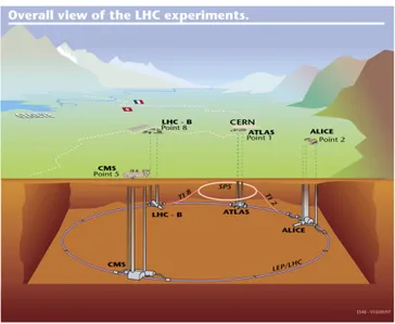
1.3 The four main experiments at LHC: ATLAS, CMS, ALICE and LHCb . . . 4
1.4 Polar angles (σ) of b and ¯b hadrons at LHC by the PYTHIA event generator . . . 7
1.5 Overview of the LHCb detector . . . 9
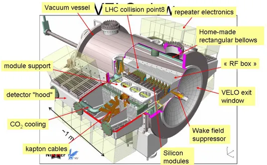
1.6 Overview of VELO . . . 11
1.7 Arrangement of the VELO modules along the beam axis . . . 12
1.8 The schematic view of R and φ silicon sensors . . . 12
1.9 Display of an average-multiplicity event in the bending plane of the tracking system, showing the reconstructed tracks and their assigned hits . . . 14
1.10 The four layers of the TT: x − u − v − x. The two middle layers are rotated ±5◦ around the z-axis to give the strips a stereo angle 15 1.11 Layout of IT x and u layer with the silicon sensors in the cross shaped configuration . . . 16
1.12 Layout of OT station (front view). In the centre the four boxes of the IT station are depicted. . . 16
1.13 Cross section of an OT module . . . 17
1.14 A cross section of the design of RICH, showing the optical path, mirrors, mirror supports . . . 19
1.16 Left: front view of a quadrant of a Muon station. Right: division into logical pads of four chambers belonging to the four regions of
station M1. . . 23
1.17 Overview of the LHCb trigger . . . 25
2.1 The architecture of LHCb Online system . . . 30
2.2 Functional block-diagram of the TELL1 readout-board. Both op-tions for the input mezzanine cards are shown for illustration. In reality the board can only be either optical or analogue. . . 32
2.3 Scope of the Experiment Control System . . . 35
2.4 The Architecture of ECS Software . . . 35
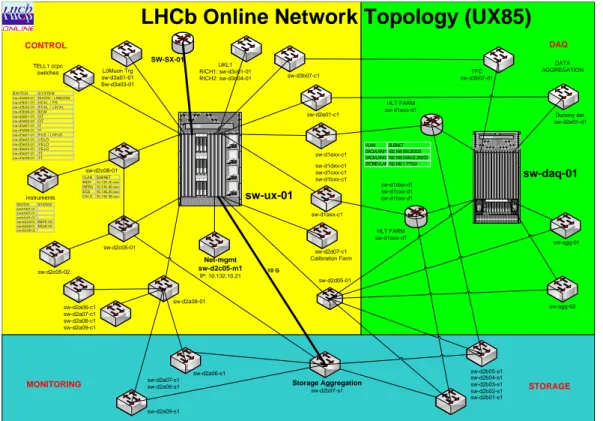
2.5 The topology of the network in the surface . . . 37
2.6 The topology of the network underground . . . 38
2.7 Tree Structure of the Control Network . . . 39
2.8 Oracle database cluster private network . . . 41
2.9 Tree Structure of the DAQ Network . . . 44
2.10 The setup for LAG performance test . . . 48
2.11 LAG performance test result . . . 49
3.1 A generic architecture of SCADA system . . . 53
3.2 Architecture of PVSS system . . . 54
3.3 Architecture of the network monitoring system . . . 57
3.4 Mechanism of DIM . . . 58
3.5 An example of MIB tree . . . 60
3.6 SNMP packet format . . . 62
3.7 Architecture of the sFlow counter collector . . . 64
3.8 Packet format of sFlow counter samples . . . 65
3.9 Example: datapoint type and datapoint . . . 66
3.10 Instances of datapoint types and datapoints . . . 66
3.11 Process of an event orientated communication connection . . . 68
3.12 Example of the topology discovery . . . 73
3.13 Uplink table . . . 76
3.14 802.3 Ethernet MAC frame . . . 77
3.16 Trending of traffic for an individual port . . . 80
3.17 Trending of traffic throughput for switches . . . 80
3.18 Monitoring of health status: F10 switch . . . 82
3.19 Status and traffic rate of external links . . . 84
3.20 FSM tree of the network monitoring system . . . 86
3.21 FSM of the DAQ network . . . 87
3.22 FSM of the uplinks in the DAQ network . . . 88
4.1 Relative estimation error . . . 92
4.2 Packet format of flow samples . . . 93
4.3 Output of “sFlowSampler” . . . 95
4.4 Architecture of daqprobe . . . 97
4.5 Database schema of “daqprobe” . . . 98
4.6 Architecture of Snort . . . 101
4.7 Snort alert list . . . 102
4.8 Snort alert detail . . . 103
5.1 Estimated time frame for LHC luminosity upgrade . . . 108
5.2 Readout architecture: new vs old . . . 110
5.3 Architecture of electronics . . . 112
5.4 X86 server forecast by Ethernet connection type . . . 113
5.5 InfiniBand roadmap . . . 116
5.6 InfiniBand architecture layers . . . 117
5.7 Top500 supercomputer interconnect: Ethernet vs InfiniBand . . . 118
5.8 Network architecture based on high-end switches . . . 123
5.9 Network architecture based on pizza-box switches: diagram of ba-sic modules . . . 124
5.10 Network architecture based on pizza-box switches: topology of modules . . . 125
5.11 Network module based on merchant networking ASICs . . . 126
5.12 Maximum buffer occupancies . . . 129
5.13 Buffer occupancy of aggregation switches . . . 130
5.15 A preliminary scheme of slot schedule to send data for readout broads . . . 131 5.16 Maximum Buffer Occupancy after optimization . . . 132 5.17 Buffer occupancy of aggregation switches after optimization . . . 132 5.18 Buffer occupancy of edge switches after optimization . . . 133
1.1 Basic design parameter values of the LHC machine . . . 4
2.1 Bandwidth Requirement . . . 43
3.1 Procedure to discover the end-nodes . . . 75
3.2 syslog Message Severities . . . 85
ACL Access Control List
ALICE A Large Ion Collider Experiment
ARP Address Resolution Protocol
ATLAS A Toroidal LHC ApparatuS
ATM Asynchronous Transfer Mode
BASE Basic Analysis and Security Engine
CAN Controller Area Network
CERN European Council for Nuclear Research
CLI Command-Line Interface
CMS Compact Muon Solenoid
COTS Commercial Off-The-Shelf
CP Charge Parity
CU Control Unit
DAQ Data Acquisition
DBM DataBase Manager
DP Data Point
DPE Data Point Element
DPT Data Point Type
DU Device Unit
ECAL Electromagnetic Calorimeter
ECS Experiment Control System
EFF Event Filter Farm
EVM Event Manager
FDB Forwarding DataBase
FEE Front-End Electronics
FPGA Field Programmable Gate Array
FSM Finite State Machine
GbE Gigabit Ethernet
GBT GigaBit Transceiver
GEM Gas Electron Multiplier
GPN General Purpose Network
HCAL Hadron Calorimeter
HLT High-Level Trigger
HMI Human Machine Interface
ICMP Internet Control Message Protocol
IDS intrusion detection system
IP Internet Protocol
IT Inner Tracker
JCOP Joint Controls Project
L0 the first level
L0DU L0 Decision Unit
LAG Link Aggregation
LAN Local Area Network
LC Line Card
LCG LHC Computing Grid
LEP Large Electron Positron
LHC Large Hadron Collider
LHCb Large Hadron Collider beauty
LINAC Linear Accelerator
LLDP Link Layer Discovery Protocol
LOM LAN-on-Motherboard
MAC Media Access Control
MAPMT Multianode Photomultiplier Tubes
NAS Network Attached Storage
NFS Network File System
NIC Networks Interface Card
ODIN Readout Supervisor
OID Object Identifier
OT Outer Tracker
PDU Protocol Data Unit
PID Particle Identification
PLC Programmable Logic Controller
PS PreShower
PS Proton Synchrotron
QDR Quad Data Rate
QSFP Quad Small Form-factor Pluggable
RDB Relational DataBase
RDMA Remote Direct Memory Access
RICH Ring Imaging Cherenkov
RMON Remote Network Monitoring
RN Readout Network
ROB Readout Board
SDR Single Data Rate
SFM Switch Fabric Module
sLHC super LHC
SM Standard Model
SMB Server Message Block
SNMP Simple Network Management Protocol
SPD Scintillator Pad Detector
SPECS Serial Protocol for ECS
SPS Super Proton Synchrotron
ST Silicon Tracker
STDIN Standard Input
STDOUT Standard Output
TCP Transmission Control Protocol
TFC Timing and Fast Control
TN Technical Network
TOE TCP/IP Offload Engine
TT Tracker Turicensis
TTL time to live
UDP User Datagram Protocol
VLAN Virtual Local Area Network
The LHCb Experiment
1.1
The Large Hadron Collider
1.1.1
The Large Hadron Collider Machine
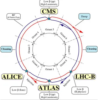
The Large Hadron Collider (LHC) [1] is the largest particle accelerator built at CERN, the European Council for Nuclear Research, straddling at the border be-tween Switzerland and France at an average depth of 100 m underground. The LHC has a 26.7 km long double-ring, and it is formed by eight arcs and eight straight sections (IRs) where the experimental regions and the utility insertions are located (see Fig. 1.1). The LHC will be capable of delivering two counter rotating proton beams at the unprecedented energy of 7 TeV each hence offer-ing collisions at a center-of-mass energy of 14 TeV. This is by far the highest achievable center-of-mass energy ever. The beams cross at a rate of 40 MHz.
The infrastructure of LHC, much of which is previously used for the Large Electron Positron (LEP), comprises the pre-acceleration system, injection system and tunnel, see Fig. 1.2. The protons are accelerated through many stages. This process starts with the Linear Accelerator (LINAC2) accelerating protons up to an energy of 50 MeV. These particles are delivered to the Proton Synchrotron Booster (PSB) which accelerates the protons up to 1.4 GeV. Then the protons are accelerated up to 26 GeV by the Proton Synchrotron (PS), and transported to the Super Proton Synchrotron (SPS). The SPS accelerates the protons to an
energy of 450 GeV. The protons are finally injected in the LHC accelerator where they reach 7 TeV in 2012.
Figure 1.1: Basic layout of the Large Hadron Collider. Beam 1 circulates clock-wise and Beam 2 counterclockclock-wise.
Figure 1.2: Schematic layout of the CERN accelerator complex
in both directions. The pipes are mainly composed of vacuum vessel, supercon-ducting dipoles and quadrupoles focusing magnets, radio-frequency accelerating cavities and cryogenic cooling. A huge cryogenic cooling system is required to maintain the liquid helium at the temperature of 1.9 K to keep the magnets cold. The beams travel in opposite directions in separate beam pipes - two tubes kept at ultrahigh vacuum, ∼ 10−4 Pa [2]. They are guided around the accelerator ring by a strong magnetic field, achieved using superconducting electromagnets. A total of 1232 magnetic dipoles with 8.4 T are used to bend the beams, and 392 quadrupole magnets are used to focus the beams [3]. The particles are accelerated close to light speed before collision in the radio-frequency cavities.
There are two important parameters for the particle accelerator: energy and luminosity. The center-of-mass energy,√s, of the collisions determines the energy available to produce new particles. The luminosity is a measure of the number of particles colliding per second per effective unit area of the overlapping beams. If two beams contains k bunches and n1 and n2 particles collide with a frequency
f , then the luminosity is defined as:
L = n1· n2· k · f
4πσ (1.1)
where σ is the beam cross-sectional area. The event rate is measured by the col-liders luminosity and is proportional to the interaction cross section. It expresses the number of particle collisions that take place every second.
The basic design parameters of the LHC machine are summarized in Table 1.1
1.1.2
The LHC Experiments
At LHC, there are four main experiments (see Fig. 1.3) run by international col-laborations, bringing together scientists from institutes all over the world. Each experiment is characterized by its unique particle detector.
• ATLAS: A Toroidal LHC ApparatuS [4]
ATLAS is one of the two general-purpose detectors at LHC. It will inves-tigate a wide range of physics, including the search for the Higgs boson, extra dimensions and particles that could make up dark matter.
Parameter Value
Proton beam energy 7 TeV
Number of bunches per beam 2808
Number of particles per bunch 1.15 x 10¹¹
Circulating beam current 0.584 A
RMS of bunch length 7.55 cm
Peak luminosity 1.0 x 1034 cm−2 s−1
Collision time interval 24.95 ns
Number of main bends 1232
Field of main bends 8.4 T
Table 1.1: Basic design parameter values of the LHC machine
Figure 1.3: The four main experiments at LHC: ATLAS, CMS, ALICE and LHCb
• CMS: Compact Muon Solenoid [5]
CMS is also a general-purpose detector and has the same scientific goals as the ATLAS experiment. It uses different technical solutions and design of its detector magnet system to achieve these. It is vital to have two inde-pendently designed detectors for cross-confirmation of any new discovery.
• LHCb: Large Hadron Collider beauty [6]
LHCb is primarily dedicated to Charge-Parity (CP) violation and rare de-cays studies in the b sector. This experiment will test the flavour sector of the Standard Model (SM) and search for new physics by making precise measurements of B meson decays.
• ALICE: A Large Ion Collider Experiment [7]
The main goal of this experiment is to produce, detect and study the nature of the quark-gluon plasma. Different from the other three experiments, AL-ICE will have Pb-Pb collisions in its interaction region. This investigation is considered fundamental to the understanding of the evolution of the early universe.
1.2
The B Physics at LHC
1.2.1
Theory Overview: CP Violation in the Standard
Model
The Standard Model of particle physics is a theory which describes the strong, weak and electromagnetic fundamental forces, as well as the fundamental particles that make up all matter: it is a quantum field theory, and consistent with both quantum mechanics and special relativity. The basic building blocks of matter are six leptons and six quarks that interact by means of force-carrying particles called bosons. Every phenomenon observed in nature should be understood as the interplay of the fundamental particles and forces of the Standard Model.
The Standard Model is a very successful theory which explains, within experi-mental precision, all experiexperi-mental phenomena yet witnessed in the laboratory and also predicts the new ones. However, it is not a definitive theory and it suffers from several limitations. First of all, it does not include gravitation, dark matter or dark energy. The essence of the mass is not resolved; whenever the mass of a particle is to be known, it has to be determined experimentally. Furthermore, the Standard Model can not explain the excess of matter over antimatter observed in the universe.
A fundamental requirement of any theory attempting to explain matter-antimatter imbalance in the early universe is that Charge-Parity (CP) symmetry could be violated. CP violation was first discovered in neutral kaon decays in 1964 [8]. Its origin is still one of the outstanding mysteries of elementary particle physics. First, CP violation in the weak interaction is generated by the com-plex three-by-three unitary matrix, known as the CKM matrix, introduced by Cabbibo [9], Kobayashi and Maskawa [10] Observed CP-violating phenomena in the neutral-kaon system are consistent with this mechanism. However, it cannot be excluded that physics beyond the Standard Model contributes, or even fully accounts for the observed phenomena. Furthermore, it is one of the three ingre-dients required to explain the excess of matter over antimatter observed in our universe. The three necessary ingredients are known as ”Sakharov conditions” proposed by Andrei Sakharov in 1967 [11].
• Baryon number B violation. • C- and CP-violation.
• Interactions out of thermal equilibrium.
The level of CP violation that can be generated by the Standard Model weak interaction is insufficient to explain the dominance of matter in the universe. This calls for new sources of CP violation beyond the Standard Model.
In the B-meson system there are many decay modes available, and the Stan-dard Model makes precise predictions for CP violation in a number of these. The B-meson system is therefore a very attractive place to study CP violation, and to search for a hint of new physics.
1.2.2
B Meson Production at LHC
LHC will be the most copious source of B mesons, compared to the other operating or under-construction machines. In LHCb, the interaction point is displaced, only 74.3% of the bunches will collide, therefore the average bunch crossing rate will be 30 MHz. The average running luminosity of the LHCb experiment has been chosen to be L = 2 · 1032cm−2s−1, in order to reduce the multiple primary pp
interactions rate and reduce the radiation damage of the detectors. Those with multiple pp interactions are much more difficult to be reconstructed than single pp interaction due to the increased particle density. At this luminosity, the effective bunch crossing rate is about 10 MHz, and a 100 kHz b¯b pair production rate is expected, hence 1012 b¯b pairs will be produced in one year.
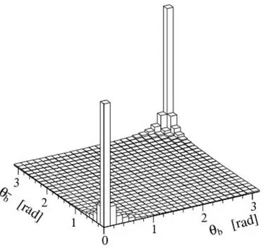
For b¯b production at LHC, the angular distribution of the b and ¯b hadrons is strongly correlated and is expected to peak in the forward directions, as is seen from the histogram in Fig. 1.4.
Figure 1.4: Polar angles (σ) of b and ¯b hadrons at LHC by the PYTHIA event generator
The b events will be a small part of the total production at LHC: σb¯b
σinel.
= 0.6% (1.2)
Therefore, in order to study b physics at LHC, a very fast and robust trigger system is required for an efficient selection of the interesting events.
1.3
The LHCb Experiment
The LHCb experiment is dedicated to the study of CP violation and other rare phenomena concerning the b quarks. Selection and reconstruction of rare B-decays in an environment with high background rates implies the following ex-perimental requirements for LHCb:
• A fast and efficient triggering scheme to reduce the large background of non-b¯b events.
• To correctly reconstruct the B mesons, a precise determination of the in-variant mass is necessary. Therefore the tracking system is designed for a high momentum resolution of typically subsection δp/p= 0.4%.
• To measure Bs oscillations, excellent vertexing and decay-time resolution is
required. The Vertex Locator (VELO) is optimized for this task and has a proper time resolution of 40 fs.
• To identify different B meson decays with identical topology, a good particle identification (PID) is necessary.
Efficient electron and Muon identification are required for trigger pur-poses and for tagging with semi-leptonic decays.
K/π separation is exploited in kaon tagging and used to separate final states which exhibits different sources of CP-violation.
Based on the expected properties of B-meson production at LHC, and taking into account the available budget and the limited space for the detector, the LHCb detector is designed as a single arm spectrometer with an angular acceptance between 10 and 300 mrad in the horizontal plane (i.e. the bending plane of the magnet), and 250 mrad in the vertical plane (non-bending plane). The LHCb detector layout is shown in Fig. 1.5. The right-handed coordinate system adopted has the z axis along the beam, and the y axis along the vertical.
LHCb comprises a vertex detector system (including a pile-up veto counter), a tracking system (partially inside a dipole magnet), aerogel and gas RICH coun-ters, an electromagnetic calorimeter with preshower detector, a hadron calorime-ter and a Muon detector. All detector subsystems, except the vertex detector,
Figure 1.5: Overview of the LHCb detector
are assembled in two halves, which can be separated horizontally for assembly and maintenance, as well as to provide access to the beam pipe.
1.3.1
The Magnet
A warm dipole magnet is used in the LHCb experiment to measure the momentum of charged particles [12]. The measurement covers the forward acceptance of ±250 mrad vertically and of ±300 mrad horizontally.The magnet is of two saddle-shaped coils in a window-frame yoke with sloping poles in order to match the required detector acceptance. Tracking detectors in the magnetic field have to provide momentum measurement for charged particles with a precision of about 0.4% for momenta up to 200 GeV/c. The design of the magnet with an integrated magnetic field of 4 Tm has to accommodate the contrasting needs for a field level inside the RICHs envelope less than 2 mT and a field as high as possible in the
regions between the vertex locator and the Trigger Tracker tracking station. A good field uniformity along the transverse coordinate is required by the Muon trigger.
1.3.2
The Vertex Locator
The VELO [13] detector system comprises a silicon vertex detector and a pile-up veto counter. Vertex reconstruction is a fundamental requirement for the LHCb experiment. Displaced secondary vertices are distinctive features of b-hadron decays. The measured track coordinates are used to reconstruct the production and decay vertices of hadrons and to provide an accurate measurement of their decay lifetimes. The VELO data are also a vital input to the High Level Trigger, informing the acquisition system about possible displaced vertices which are a signature of the B-mesons in the event. The High Level Trigger requires all channels to be read out within 1 µs. The pile-up veto counter is used in the first level (L0) trigger to suppress events containing multiple pp interactions in a single bunch-crossing, by counting the number of primary vertices.
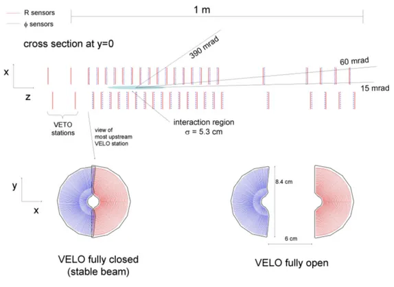
The VELO is composed of a series of silicon detector stations placed along the beam direction. They are positioned at a radial distance from the beam which is smaller than the aperture required by LHC during injection and therefore must be retractable. This is achieved by mounting the detectors in a setup similar to Roman pots, see Fig. 1.6.
The layout of the VELO and the pile-up veto stations is shown in Fig. 1.7. Each station is made of two planes of sensors, measuring the radial and the angu-lar components of all tracks. Apart from covering the full LHCb forward anguangu-lar acceptance, the VELO also has a partial coverage of the backward hemisphere to improve the primary vertex measurement. To facilitate the task of the L0 trigger to select events with only one p-p interaction per bunch crossing, two additional R sensors are placed upstream of the VELO stations forming the pile-up veto stations.
The LHCb VELO silicon sensors are very complex devices. Both R and φ sensors are shown in Fig. 1.8. They are made of 300 µm thick n-on-n single sided
Figure 1.6: Overview of VELO
silicon wafers with AC coupling to the readout electronics covering the angle of 182◦, including a 2◦ overlap area with the opposite sensor.
The strips in the R-sensor are concentric semi-circles segmented into four 45◦ sectors. Each sector has 512 strips. The radial coverage of sensor varies from the inner radius of ∼8.2 mm to the outer radius of ∼ 41.9 mm. The pitch between individual strips increases linearly with the radius from 40.0 µm to 101.6 µm.
The strip orientation in the φ sensor is semi-radial. The sensor is divided into an inner and an outer region. The inner and outer regions contains 683 and 1365 strips respectively, chosen to equalize the occupancy in the two regions. The pitch of the inner region varies from 35.5 µm to 78.3 µm and of the outer region from 39.3 µm to 96.6 µm. The sensors are flipped from station to station and the strips are tilted with a stereo angle, which is different in sign and magnitude for the inner and outer region.
Figure 1.7: Arrangement of the VELO modules along the beam axis
Figure 1.8: The schematic view of R and φ silicon sensors
x and y. For secondary vertices the spatial resolution depends on the number of tracks but on average it varies from 150 to 300 µm in z. This roughly corresponds
to a resolution of 50 fs for the B-lifetime.
1.3.3
Tracking
The LHCb tracking system is used together with the VELO detector to recon-struct charged particle tracks within the detector acceptance. The LHCb tracking system consists of four planar tracking stations: the Tracker Turicensis (TT) up-stream of the dipole magnet and T1-T3 downup-stream of the magnet. TT uses silicon microstrip detectors. In T1-T3, silicon microstrips are used in the region close to the beam pipe (Inner Tracker, IT), whereas straw-tubes are employed in the outer region of the stations (Outer Tracker, OT). The TT and the IT were developed in a common project called the Silicon Tracker (ST).
In LHCb, charged particle trajectories are reconstructed by the Vertex detec-tor placed at the interaction point and by the Tracking stations. The simulation is shown in Fig. 1.9. The magnet provides bending power for charged particles to allow particle momentum measurements. The tracking stations provide mea-surements of track coordinates for momentum determination in the horizontal bending plane of the magnet and sufficient resolution for pattern recognition in the vertical coordinate.
1.3.3.1 Trigger Tracker
The Trigger Tracker (TT) [14] is located downstream of RICH1 and in front of the entrance of the LHCb magnet. It fulfills a two-fold purpose. Firstly, it will be used in the High Level trigger to assign transverse-momentum information to large-impact parameter tracks. Secondly, it will be used in the offline analysis to reconstruct the trajectories of long-lived neutral particles that decay outside of the fiducial volume of the Vertex Locator and of low-momentum particles that are bent out of the acceptance of the experiment before reaching tracking stations T1T3.
TT consists of two stations separated by a distance of 27 cm, and each station has two layers of silicon covering the full acceptance. The strips in the four layers are arranged in stereo views, x-u and v-x, corresponding to angles with the vertical y axis of 0◦, 5◦, +5◦ and 0◦. The stereo views allow a reconstruction
Figure 1.9: Display of an average-multiplicity event in the bending plane of the tracking system, showing the reconstructed tracks and their assigned hits
of tracks in three dimensions. The vertical orientation of the strips is chosen to obtain a better spatial resolution in the horizontal plane (bending plane of the magnet), resulting in a more accurate momentum estimate.
A layer is built out of 11 cm × 7.8 cm sensors as depicted in Fig. 1.10. The active area of the station will be covered entirely by silicon microstrip detectors with a strip pitch of 198 µm and strip lengths of up to 33 cm, the silicon sensors cover a surface of about 8.4 m2 in total. Depending on their distance from the
horizontal plane, the strips of three or four sensors are connected so that they can share a single readout. The spatial resolution is ∼50 µm by clustering neighboring strips.
1.3.3.2 Inner Tracker
The Inner Tracker (IT) [15] covers the innermost region of the T1, T2 and T3 stations, which receives the highest flux of charged particles. It consists of four
Figure 1.10: The four layers of the TT: x − u − v − x. The two middle layers are rotated ±5◦ around the z-axis to give the strips a stereo angle
cross-shaped station equipped with silicon sensors, placed around the beam. The silicon foils are 300 µm thick and have a 230 µm strip pitch, resulting in a reso-lution of approximately 70 µm.
An IT station consists of four boxes of silicon sensors, placed around the beam pipe in a cross-shape. It spans about 125 cm in width and 40 cm in height (see Fig. 1.11). Each station box contains four layers in an x − u − v − x topology similar to that in the TT. The silicon sensors have the same dimensions as in the TT. The strip pitch is 198 µm, resulting in a resolution of approximately 50 µm.
Figure 1.11: Layout of IT x and u layer with the silicon sensors in the cross shaped configuration
1.3.3.3 Outer Tracker
The Outer Track [16] is a straw tube detector which complements the IT by covering the remaining LHCb acceptance in T1, T2 and T3 station, as shown in Fig. 1.12. It is similarly laid out, with each of the three tracking stations having= four straw tube OT layers associated with it, arranged in the same manner (x − u − v − x) as those of the TT and IT.
Figure 1.12: Layout of OT station (front view). In the centre the four boxes of the IT station are depicted.
The layout of the straw-tube modules is shown in Fig. 1.13. The modules are composed of two staggered layers (monolayers) of 64 drift tubes each. In the longest modules (type F) the monolayers are split longitudinally in the middle into two sections composed of individual straw tubes. Both sections are read out
from the outer end. In addition to the F-type modules there exist short modules (type S) which are located above and below the beam pipe. These modules have about half the length of F-type modules, contain 128 single drift tubes, and are read out only from the outer module end. The inner diameter of the straws is 5.0 mm, and the pitch between two straws is 5.25 mm. As a counting gas, a mixture of Argon (70%) and CO2 (30%) is chosen in order to guarantee a fast
drift time (below 50 ns), and a sufficient drift-coordinate resolution (200 µm). The gas purification, mixing and distribution system foresees the possibility of circulating a counting gas mixture of up to three components in a closed loop.
Figure 1.13: Cross section of an OT module
1.3.4
Particle Identification
Particle identification (PID) is a fundamental requirement for LHCb, and it is provided by the two Ring Imaging Cherenkov (RICH) detectors, the Calorimeter system and the Muon Detector.
For the common charged particle types (e, µ, π, K, p), electrons are primarily identified using the Calorimeter system, muons with the Muon Detector, and hadrons with the RICH system. However, the RICH detectors can also help improve the lepton identification, so the information from the various detectors is combined. Neutral electromagnetic particles (γ, π0) are identified using the
Calorimeter system, where the π0 → γγ may be resolved as two separate photons, or as a merged cluster. Finally K0
S are reconstructed from their decay KS0 →
π+π− [14]. These various particle identification techniques are described in the
following sections.
1.3.4.1 The RICH
The main aim of the RICH detectors is hadron identification in LHCb, especially the separation of pions from kaons [17]. The Cherenkov radiation phenomenon is exploited in the RICH detectors in order to perform particle identification. When charged particles pass through a transparent medium at a constant speed greater than the speed of light in that medium, Cherenkov radiation is emitted at a constant angle, the Cherenkov angle θc, to the direction of motion of the
particle. The Cherenkov angle depends only on the speed of the particle and is given by [18]
cos θc'
1 β0n
(1.3) where n is the refractive index of the medium, β0 = v/c is the initial velocity
fraction of the radiating particle.
Both detectors measure the Cherenkov angle. At large polar angles the mo-mentum spectrum is softer while at small polar angles the momo-mentum spectrum is harder. To cover the full momentum range, this is accomplished by two Ring Imaging Cherenkov detectors. The upstream detector, RICH1, covers the low momentum charged particle range ∼1 - 60 GeV/c using aerogel and C4F10 radi-ators, while the downstream detector, RICH2, covers the high momentum range from ∼15 GeV/c up to and beyond 100 GeV/c using a CF4 radiator. Overview of RICH1 and RICH2 are shown in Fig. 1.14a and Fig. 1.14b.
In both RICH detectors the focusing of the Cherenkov light is accomplished using a combination of spherical and flat mirrors to reflect the image out of the spectrometer acceptance. Hybrid Photon Detectors (HPDs) are used to detect the Cherenkov photons in the wavelength range 200 - 600 nm. The HPDs are surrounded by external iron shields and are placed in MuMetal cylinders to per-mit operation in magnetic fields up to 50 mT. The angular distribution of the
(a) RICH1 (b) RICH2
Figure 1.14: A cross section of the design of RICH, showing the optical path, mirrors, mirror supports
Cherenkov radiation emitted by a charged particle is related to the velocity of the particle.
A particle is identified by its rest mass and electric charge. The electric charge is determined by the bending of the particle trajectory in the magnetic field. Combining the measurement of the velocity performed by the RICH detectors with the momentum from the tracking system and the magnetic field, one is able to identify the ultra-relativistic particles. The velocity of a particle is related to the angular distribution of the Cherenkov radiation emitted by the charged particle. The resolution on the reconstructed Cherenkov angle has the following contributions: emission point, chromatic dispersion of the radiators, pixel of the photon detector and the tracking.
1.3.4.2 The Calorimeter System
The calorimeter system performs several functions. It selects transverse energy hadron, electron and photon candidates for the L0 trigger, which makes a decision 4µs after the interaction. It provides the identification of electrons, photons
and hadrons as well as the measurement of their energies and positions. The reconstruction with good accuracy of π0 and prompt photons from the primary interactions is essential for flavour tagging and for the study of B-meson decays and therefore is important for the LHCb physics program [6].
To meet the fast triggering requirements, the chosen structure for the calorime-ter system consists of three elements: a Scintillator Pad Detector and single-layer Preshower (SPD/PS) detector, followed by a Shashlik electromagnetic calorime-ter (ECAL) and a scintillating tile hadron calorimecalorime-ter (HCAL).
• The Scintillator Pad Detector (SPD) identifies charged particles by means of 15 mm-thick scintillator tiles, which allow to separate photons from elec-trons. The light produced by a ionizing particle traversing the tiles is col-lected by Wavelength Shifting Fibers (WLS). The re-emitted green light is guided outside the detector acceptance towards the channel Multianode Photomultiplier Tubes (MAPMT) via clear plastic fibers. All the calorime-ter detectors follow the same basic principle: scintillation light is transmit-ted to a Photomultiplier Tubes by wavelength shifting fibers. The SPD is followed by the PreShower detector that consists of 12 mm-thick lead plane placed in front of 15 mm-thick scintillator plane. The lead plates allow electrons to interact and hence produce an extra shower before reaching the scintillator plates.
• The electromagnetic calorimeter adopts the shashlik calorimeter technol-ogy [19], i.e. a sampling scintillator/lead structure readout by plastic WLS fibers. ECAL is realized as a rectangular wall constructed out of 3312 sep-arate modules of square section. It is subdivided into three sections, Inner, Middle and Outer, comprising modules of the same size but different gran-ularities. The performance of ECAL should comply with the following list of specifications [20].
* an energy resolution σE/E(GeV ) on the level of 10%/√E ⊕ 1% * a fast response time compatible with LHC bunch spacing 25 ns • The LHCb hadron calorimeter (HCAL) is a sampling device made from
The special feature of this sampling structure is the orientation of the scin-tillating tiles that run parallel to the beam axis. In the lateral direction tiles are interspersed with 1 cm of iron, whereas in the longitudinal direction the length of tiles and iron spacers corresponds to the hadron interaction length λI in steel. The energy resolution is:
σ(E)
E =
80% √
E ⊕ 10% (E in GeV ) (1.4)
1.3.4.3 The Muon Detector
Muon triggering and offline Muon identification are fundamental requirements of the LHCb experiment. Muons are present in the final states of many CP-sensitive B decays, in particular the two gold-plated decays, B0d → J/ψ(µ+µ−)K0 S
and Bd0 → J/ψ(µ+µ−)φ [14]. They play a major role in CP asymmetry and
oscillation measurements, since muons from semi-leptonic b decays provide a tag of the initial state flavor of the accompanying neutral B mesons. In addition, the study of rare B decays such as the flavour-changing neutral current decay, B0
d → µ+µ
−, may reveal new physics beyond the Standard Model [6].
Muon particles with high transverse momentum are typical signatures of a b-hadron decay, and the Muon system provides fast information for the high-PT
Muon trigger at the first level (L0) and Muon identification for the high-level trigger (HLT) and offline analysis.
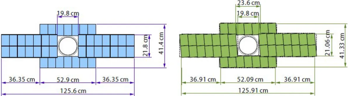
The Muon system [21], shown in Fig. 1.15, is composed of five stations (M1-M5) of rectangular shape, placed along the beam axis. The full system comprises 1380 chambers and covers a total area of 435 m2. The inner and outer angular acceptances of the Muon system are 20 (16) mrad and 306 (258) mrad in the bending (non-bending) plane respectively. Station M1 is placed in front of the calorimeters and is used to improve the PT measurement in the trigger. Stations
M2 to M5 are placed downstream the calorimeters and are interleaved with iron absorbers 80 cm thick to select penetrating muons. The minimum momentum of a Muon to cross the five stations is approximately 6 GeV/c since the total absorber thickness, including the calorimeters, is approximately 20 interaction lengths.
Figure 1.15: Side view of the Muon system
In the innermost region of the first Muon station, Gas Electron Multiplier (GEM) detectors have been adopted, because the innermost region is exposed to a high particle rate, which reaches the values of about 230 kHz/cm2 at the nominal
lu-minosity value. Multi-Wire Proportional Chambers (MWPC) have been adopted as the baseline detector in all the other regions where the expected particles rates are lower.
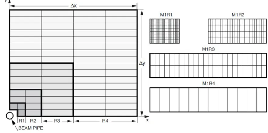
Further, each Muon Station is divided into four regions, R1 to R4 with in-creasing distance from the beam axis, as show in Fig. 1.16. The linear dimensions of the regions R1, R2, R3, R4, and their segmentations scale according to the ratio 1:2:4:8.
To provide a high-pT Muon trigger at the L0 trigger with a 95% efficiency
within a latency of 4.0 µs, each station has a time resolution sufficient to give a 99% efficiency within a 20 ns time window. The Muon system unambiguously identifies the bunch crossing which generated the detected muons, and then selects
Figure 1.16: Left: front view of a quadrant of a Muon station. Right: division into logical pads of four chambers belonging to the four regions of station M1.
the Muon track and measure its pT with a resolution of 20%.
1.3.5
The LHCb Trigger and DAQ
The LHC bunches cross at a rate of 40 MHz. LHCb will operate at a luminosity of 2 × 1032cm−2s−1, about fifty times less than the LHC design luminosity. At the lower operating luminosity, the LHCb spectrometer will have only 10 MHz of crossings with “visible interactions”, defined as interactions that produce at least two charged particles with sufficient hits to be reconstructed in the spectrome-ter [22, 23].
At the nominal luminosity of LHCb, the bunch crossings with visible pp in-teractions are expected to contain a rate of about 100 kHz of bb-pairs. However, only about 15% of these events will include at least one B meson with all its decay products contained in the spectrometer acceptance. Furthermore the branching ratios of interesting B meson decays used to study for instance CP violation are typically less than 103. The offline analysis uses event selections based on the masses of the B mesons, their lifetimes and other stringent cuts to enhance the signal over background.
Fig. 1.17 is the overview of the LHCb trigger system, showing the triggers and the expected trigger rate, and the the sub-detectors participating involved. The trigger is based on a two-level system and exploits the fact that b-flavoured
hadrons are heavy and long-lived. The first level (L0), is implemented in custom hardware. Its main goal is to select high transverse energy, ET , particles using
partial detector information. The L0 trigger reduces a rate of 10 MHz of crossings with at least one visible interaction to an output rate of 1 MHz.
After a L0 accept, all the detector information is then read out and fed into the High Level Trigger (HLT). This software trigger runs in the event-filter farm composed of about 1700 CPU nodes. From the HLT, events are selected at a rate of 2 kHz and sent for mass storage and subsequent offline reconstruction and analysis.
1.3.5.1 The L0 Trigger
The L0 trigger is a custom hardware trigger system, its purpose is to reduce the LHC beam crossing rate to 1 MHz. The main goal of the L0 trigger is three-fold: • to select high ET particles: hadrons, electrons, photons, neutral pions and
muons;
• to reject complex/busy events which are more difficult and take longer to reconstruct;
• to reject beam-halo events.
The level-0 trigger uses information from the calorimeter system, the Muon chambers and the pile-up system.
• The pile-up system provides rejection of events by identifying bunch cross-ings with multiple primary vertices. Two-interaction crosscross-ings are identified with an efficiency of 60% and a purity of about 95%. [23]
• The calorimeter system provides candidate hadrons, electrons, photons and neutral pions. The calorimeter system outputs to the L0 decision unit (L0DU) the highest ET hadron, electron, photon and π0 candidates, and
the total HCAL ET and SPD multiplicity.
• The Muon chambers allow stand-alone Muon reconstruction with a pT
res-olution of 20%. The two highest pT muon candidates from each quadrant
The L0 decision unit combines the output from these three components and issues the final trigger decision. This decision is passed to the Readout Supervisor which transmits its L0 decision to the Front-End Electronics (FEE). The latency of the L0 trigger is 4µs.
1.3.5.2 The High-Level Trigger
The High Level Trigger (HLT) is fully implemented in software, it consists of a C++ application which runs on every CPU of the Event Filter Farm (EFF). The EFF contains up to 2000 computing nodes. The HLT is very flexible and will evolve with the knowledge of the first real data and the physics priorities of the experiment. In addition the HLT is subject to developments and adjustments following the evolution of the event reconstruction and selection software.
The HLT is subdivided in two stages, HLT1 and HLT2. HLT1 applies a progressive, partial reconstruction seeded by the L0 candidates. Different recon-struction sequences (called alleys) with different algorithms and selection cuts are applied according to the L0 candidate type. HLT1 should reduce the rate to a sufficiently low level to allow for full pattern recognition on the remaining events, which corresponds to a rate of about 30 kHz. HLT1 starts with so-called alleys, where each alley addresses one of the trigger types of the L0 trigger. The combined output rate of events accepted by the HLT1 alleys is sufficiently low to allow an off-line track reconstruction. At this rate HLT2 performs a combination of inclusive trigger algorithms where the B decay is reconstructed only partially, and exclusive trigger algorithms which aim to fully reconstruct B hadron final states.
The HLT reduce the rate to about 2 kHz, the rate at which the data is written to storage for further analysis.
1.3.5.3 Data Acquisition
The role of the Data Acquisition (DAQ) system is to transport the event frag-ments, selected by L0DU, from the front-end electronics (FEE) to the HLT farm. First, the data are readout and buffered in the front-end electronics during the latencies of the hardware triggers. The selected events will be sent to the readout
boards, called TELL1 or UKL1, where the front-end links are multiplexed and event fragments are assembled and zero-suppressed. Then the data are sent to the Readout Network (RN), then are transported to a node in the HLT farm. The details of DAQ system will be described in chapter 2.
1.4
Summary
The LHCb experiment is one of the four large particle detectors running at the Large Hadron Collider accelerator at CERN. It is a forward single-arm spec-trometer dedicated to test the Standard Model through precision measurements of CP violation and rare decays in the b quark sector. In this chapter, all the sub-detectors and the trigger and DAQ system of LHCb were described, from structures to expected performances. More information can be found in the pa-per [6].
The LHCb Online System and Its
Networks
The Online system is a key part of the LHCb experiment. It comprises all the IT infrastructure (both hard- and software). The main task of the Online system is to operate the experiment, and transport data from the front-end electronics to permanent storage for physics analysis. This includes not only the movement of the data themselves, but also the configuration of all operational parameters, their monitoring and the control of the entire experiment. The Online system also must ensure that all detector channels are properly synchronized with the LHC clock [24, 25]. The architecture of LHCb Online system is shown in Fig. 2.1.
The LHCb Online system consists of three subsystems:
• the Data Acquisition (DAQ) system: to collect the event fragments orig-inating from front-end electronics and transport the data belonging to a given bunch crossing, identified by the trigger, to permanent storage. • the Timing and Fast Control (TFC) system: to synchronise the entire
read-out of the LHCb detector between the front-end electronics and the Online processing farm by distributing the beam-synchronous clock, the Level-0 trigger, synchronous resets and fast control commands.
• the Experiment Control System (ECS): to monitor and control the opera-tional state of the LHCb detector. This includes the classical “slow” control,
SWITCH HLT farm Detector TFC System SWITCH
SWITCH SWITCH SWITCH SWITCH SWITCH
READOUT NETWORK L0 trigger LHC clock MEP Request Event building Front-End C P U C P U C P U C P U C P U C P U C P U C P U C P U C P U C P U C P U C P U C P U C P U C P U C P U C P U C P U C P U C P U C P U C P U C P U Readout Board
VELO ST OT RICH ECal HCal Muon
L0 Trigger
Event data
Timing and Fast Control Signals Control and Monitoring data
SWITCH MON farm C P U C P U C P U C P U Readout
Board Readout Board Readout Board Readout Board Readout Board Readout Board
FEE FEE FEE FEE FEE FEE FEE
CASTOR
Figure 2.1: The architecture of LHCb Online system
such as high and low voltages, temperatures, gas flows and pressures, and also the control and monitoring of the Trigger, TFC and DAQ systems (traditionally called “run-control”).
2.1
Data Acquisition
2.1.1
Physics Requirements
The DAQ is responsible for the data taking from the front-end electronics to the HLT farm. Reliability and efficiency are expected from the DAQ system in order to record as many interesting events as possible.
For the events selected by the L0 trigger, the entire detector is read out, because LHCb physics requires the full event data. The data acquisition system
should ensure the error-free transmission of the data from the front-end electronics to the HLT farm, and then to the storage device. This data transfer should not introduce any dead-time, if the system is operated within the design parameters.
2.1.2
Data Readout
As shown in Fig. 2.1, the data acquisition is composed of the following major components:
• Front-end Electronics (FEE) and Readout Boards • Readout Network
• HLT CPU Farm
There are two kinds of readout-links in LHCb, the front-end electronics of VELO sends the data over analogue cables and digitizes them only at the input of the readout boards, while the other detectors digitize the signal in the front-end electronics and transmit them over optical fibres. Here the description of the front-end readout is based on the latter, but almost everything applies as well to VELO. First the front-end electronics captures the analogue signals from the detectors and converts them into digital data which are then stored in a 160 cells deep L0 buffer pipeline at 40 MHz. As had been explained in Section 1.3.5.1, the signals from the calorimeters, the MUON and the Pile-Up sub-detectors are in addition sent to the L0 trigger system. Thereafter, the L0 decision is sent to the output stage of the L0 buffer pipeline. According to the decision received, data is either rejected or written to the L0 derandomizer in order to adapt the rate of data transmission to the capacity of the front-end links. The maximum delay allowed is 4.0 µs (160 clocks).
The front-end electronics feeds the events selected by L0 trigger into 330 Readout Boards (TELL1/UKL1) [26] via approximately 5000 optical links, each link has a maximum raw band-width of 160 MB/s. The data are processed in four pre-processing FPGAs(Field Programmable Gate Array), where common-mode processing, zero-suppression or data compression is performed depending on the needs of individual detectors. The resulting data fragments are collected by a
fifth FPGA (SyncLink) and formatted into a raw IP-packet that is subsequently sent to the readout network via the 4-port GbE(Gigabit Ethernet) mezzanine card. The data rate is reduced by a factor 4 to 8, depending on the attached sub-detector. A block-diagram of the TELL1 board is shown in Fig. 2.2
Figure 2.2: Functional block-diagram of the TELL1 readout-board. Both options for the input mezzanine cards are shown for illustration. In reality the board can only be either optical or analogue.
A simple dataflow protocol is used on the readout network. It is based push paradigm with central load-balancing and flow-control. Data is transferred to the next stage when some new data is available. The data flow is supervised by the central readout supervisor (“ODIN”). There is no synchronization or communica-tion between components of the same horizontal level. Any data-sink (server-PC in the farm) declares its availability to the readout supervisor, which then sends trigger commands and destination broadcasts to the readout boards.
A custom network transport protocol was defined for the data transfer from the readout boards to farm-nodes, which is called Multi-Eventfragment Proto-col [27]. This is a lightweight, unreliable datagram protoProto-col over IP similar to the User Datagram Protocol (UDP). There is no retransmission mechanism.
The event size in LHCb is quite small, on average every Readout Board will have only ∼ 100 bytes per trigger. The Multi-Eventfragment Protocol allows to assemble the data from multiple events into a multi-event packet (MEP) in order to reduce the overhead from protocol headers and to mitigate the packet rate at the receiving nodes. In the Multi-Eventfragment Protocol, the packing factor, namely the number of events in a single MEP, can be tuned to gain a better efficiency.
For the event building, the CPU farm nodes announce their availability to receive MEPs by sending MEP Requests to ODIN when the local event queue contains less than a certain number of events. ODIN thus assigns the destinations of the MEPs dynamically according to the availability of the farm nodes. The destinations are broadcast to the TELL1 readout boards over the TTC system, along with other information, i.e. packet factor, and event ID.
All the data are forwarded in an Ethernet network, which is described in Section 2.3.2.
2.1.3
High Level Trigger and Data Storage
In the CPU farm, the HLT algorithm selects interesting interactions; upon a positive decision, the data are subsequently sent to permanent storage. The HLT is expected to reduce the overall rate from the original trigger rate of 1 MHz to ∼ 2 kHz by a factor of 500. As shown in Fig. 2.1, accepted events are sent off the farm nodes, routed by the edge switch (also called access switch) to the LHCb Online storage cluster, where all the selected events are written into raw data files. The size of the raw data file is normally ∼2 GB. The raw data files are registered in a run-database and transferred to the CERN mass-storage facility CASTOR as soon as they are closed. The storage system has a capacity of ∼ 40 TB, which should offer sufficient buffer space to cope with possible interruptions of the transfer to permanent storage at CERN. For security reasons, a firewall is deployed in the LHCb Online network. Only a few trusted nodes in the CERN computing center are allowed to access the LHCb Online storage cluster.
2.2
The Experiment Control System
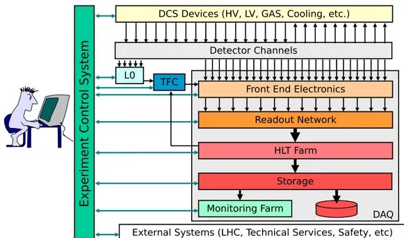
The LHCb Experiment Control System (ECS) will handle the configuration, mon-itoring and operation of all experiment equipments involved in the different activi-ties of the experiment. This encompasses not only the traditional detector control domains, such as high and low voltages, temperatures, gas flows, or pressures, but also the control and monitoring of the Trigger, TFC and DAQ systems [24, 28]. The scope of LHCb ECS is shown in Fig. 2.3
• Data acquisition and trigger (DAQ): Timing, frontend electronics, readout network, Event Filter Farm, etc.
• Detector operations (DCS): Gases, high voltages, low voltages, tempera-tures, etc.
• Experimental infrastructure: Magnet, cooling, ventilation, electricity dis-tribution, detector safety, etc.
• Interaction with the outside world: LHC Accelerator, CERN safety system, CERN technical services, etc.
The ECS software is based on PVSS II [29], a commercial SCADA (Super-visory Control And Data Acquisition) system. A common project: the Joint Controls Project (JCOP) [30] has been setup between the four LHC experiments to define a common architecture and a framework to be used by the experiments in order to build their control systems. This toolkit provides components needed for building a homogeneous ECS system, and facilitates integrating the sub-systems coherently. Based on this framework, a hierarchical and distributed system was designed as depicted in Fig. 2.4.
The ECS is organized in a tree, where parent-nodes “own” child-nodes and send commands to them. Children send “states” back to their parents. Nodes are of two types:
• Device Units: which are capable of driving the equipment to which they correspond1.
Detector Channels
Front End Electronics Readout Network HLT Farm Storage L0 E x p e ri m e nt C ont rol S y st e m DAQ DCS Devices (HV, LV, GAS, Cooling, etc.)
External Systems (LHC, Technical Services, Safety, etc) TFC
Monitoring Farm
Figure 2.3: Scope of the Experiment Control System
LV
Dev1 LVDev2 LVDevN
DCS SubDetN DCS SubDet2 DCS SubDet1 DCS SubDet1 LV SubDet1 TEMP SubDet1 GAS
…
…
C om m an ds DAQ SubDetN DAQ SubDet2 DAQ SubDet1 DAQ SubDet1 FEE SubDet1 RO FEEDev1 FEEDev2 FEEDevN
Control Unit Device Unit