The Evolution of the Lead-lag Markets in the Price Discovery Process of the Sovereign Credit Risk: the Case of Italy

(1)

https://doi.org/10.47260/jafb/1127 Scientific Press International Limited

The Evolution of the Lead-lag Markets in the Price

Discovery Process of the Sovereign Credit Risk:

the Case of Italy

Michele Anelli1, Michele Patanè2, Mario Toscano3 and Alessio Gioia4

Abstract

Hedging and speculative strategies play a key role in periods of financial market volatility particularly during economic crises. In such contexts, liquidity problems tend to evolve into potential credit risk events that amplifies the volatility of several markets such as the CDS and the government bond markets. The former, however, generally embodies a higher sensitivity to volatility due to the operators’ uncertainty about unstable and countercyclical counterparty risk.

The aim of this paper is to analyze the long-lasting dynamic relationship between credit default swap (CDS) premia and government bond yield spreads (GBS), by focusing particularly on sovereign credit risk, in order to evaluate the lead-lag markets in the price discovery process against the backdrop of a deep financial crisis. The focus of this study concerns the country of Italy, one of the major European countries that suffers from both weak GDP growth and high public debt, which subjects it to volatility and speculation during periods of financial stress.

JEL classification numbers: G01, G12, G14, G20.

Keywords: CDS spreads, Government bond spreads, Credit risk, Cointegration, Vector error correction model, Granger-causality.

1_{PhD, Department of Economics and Statistics, School of Economics and Management,}

University of Siena, Siena, Italy.

2_{Associate Professor, Department of Business and Law, School of Economics and Management,}

University of Siena, Siena, Italy.

3_{PhD, Department of Business and Law, School of Economics and Management, University of}

Siena, Siena, Italy.

4_{Portfolio Manager and Financial Analyst, Mantova, Italy.}

Article Info: Received: January 6, 2021. Revised: January. 24, 2020.

(2)

1. Introduction

In this empirical study, we analyze the connection between a time series of government bond spreads, calculated as the differential between the ten-years Italian government bond (BTP) yield and the respective German government bond (Bund) yield, and ten-years Italian CDS spreads (or premia) in order to evaluate their different ability to immediately incorporate information on credit risk, specifically for the case of Italy. Why do we focus specifically on Italy? Italy is an industrialized country that holds a prominent position in Europe as well as in the world. During the sovereign debt crisis, Italy has been (and it continues to be) considered as one member of the so-called “PIIGS”, which are the peripheral countries of the Eurozone. Portugal, Italy, Ireland, Greece and Spain were harshly hit by financial crisis. The Italian case, however, is particularly interesting in this study for four main reasons:

1) Italy (as well as Spain) was close to the default in 2011, notwithstanding the presence of a solid industrial structure;

2) Italy is characterized by a high public debt, weak growth expectations and political fragility;

3) Italian government bonds represent one of the main strategic components held in the portfolios of Italian banks (Longo, 2018);

4) the Italian bond market is one of the most liquid and efficient market worldwide with a large presence of foreign dealers and investors (MEF, 2017).

Why do we focus on the evolution of the price discovery process of the credit risk by disentangling a decade of crisis/low inflation? We try to analyze, step-by-step, market interdependencies and show how they can dynamically adjust and reverse over time. The concept of “long-term relationship” has a relative meaning in financial markets. Keynes’ famous observation “in the long-run we are all dead” probably is the best way to make the idea. In general, long-term mean-reversion phenomena can offer trading margins to make profits while minimizing risk for financial operators. The CDS is one of the typical instrument that measures the credit risk of the reference entity, and is used to implement both hedging and speculative strategies. For corporate as well as sovereign CDSs, the CDS spread can be interpreted as a credit spread on a bond issued by the reference entity. According to Duffie (1999), the CDS premium should be equal to the yield spread over a risk-free benchmark on a par floating-rate bond. The government bond spread (GBS) is the differential with respect to the risk-free rate (i.e., AAA rating) and it embodies different typology of risks (e.g., liquidity risk), not only the credit risk. Many studies, indeed, show that credit risk is not the only determinant and that other kinds of risk play a fundamental role in this sense (Elton et al., 2002; Hull et al., 2004; Fontana et al., 2016). However, if credit risk is the main factor that is priced, what we should find is a close co-movement of these series. Therefore, by following this perspective, the fundamental assumption is that the main priced factor is credit risk.

(3)

2. Literature Review

There is extensive literature about sovereign credit risk, as several authors have already investigated the relationship between CDS premia and bond spreads. In particular, most of these authors focused on the so-called “CDS-bond basis”, that is the differential between the CDS premium and the bond spread. Duffie (1999) was the first author to claim that a perfect correspondence exists, and that there are no chances of arbitrage, between a risky bond asset, a risk-free bond asset and a CDS instrument with the same expiry and an equal notional value. In normal market conditions, the CDS-bond basis generally tends to be approximately equal to zero5. However, in more turbulent market backdrops, it can differ from zero and create arbitrage strategies as Amadei et al. (2011) point out. Also with the aim of investigating the drivers that cause the violation of the arbitrage opportunities absence, Bai et al. (2011) investigate both the time-series and cross-sectional variation in the CDS-bond basis during the Financial Crisis of 2007-2009 in the U.S. market. One of their results is that the share of price-discovery occurring in the CDS market falls significantly during the crisis. With particular focus on one of the highest volatility periods and Euro Area, Fontana et al. (2016) compare the market pricing of Euro Area government bonds and the corresponding CDSs by analyzing the basis (defined as the difference between the premium on the CDS and the credit spread on the underlying bond) during the period from January 2007 to December 2012. Gyntelberg et al. (2016) try to explain the persistent non-zero CDS-bond basis in Euro Area sovereign debt markets and its increase during the last sovereign crisis. Other authors, rather, have investigated on the price discovery process of the credit risk and on the different markets ability promptly to incorporate the dynamics of the credit risk. Our paper focuses on this specific last aspect. Lehmann (2004) defines the “price discovery analysis of credit risk” as the efficient and prompt integration of new information implicitly discounted in market prices. The existence of multiple linked markets in which the risky bond asset is traded implies that the total information flow is spread over these markets; thereafter an intermarket analysis is particularly essential for forecasting purposes (to determine which market anticipates the other?). Coudert et al. (2010) analyze the links between credit default swaps (CDSs) and (corporate and government) bonds and try to determine which is the leader in the price discovery process over the period 2007-2010. The bond spread is calculated as the difference between the bond yield and a risk-free rate. They consider a 5-year risk-free rate by area, such as the German Bund for the European Union, gilts for the United Kingdom, and the US Treasury bond for other areas. The results show that the CDS market has a lead on the bond market in the price discovery process for corporates as well as sovereigns taken as a whole. For corporates, this is in line with the greater liquidity of the CDS market, while for sovereigns results are more challenging as the size of the CDS market is relatively

5_{In reality, bond and CDS spreads are never equal for a number of reasons, such as accrued interest,}

the cheapest-to-deliver option and counterparty risk among other factors. Market liquidity also plays a key role in the gap between the two spreads (Coudert et al., 2010).

(4)

small compared with the debt market. Data shows that the lead of the CDS market only holds for high-yield countries (it is particularly pronounced in emerging areas) and the government bond market still leads the CDS spreads in low-yield countries. Palladini et al. (2011) test the price discovery relationship between sovereign CDS premia and bond yield spreads on the same reference entity. Their study is focused on the Euro Area countries over the period 2004-2011. The VECM analysis suggests that the CDS market leads the bond market in the price discovery process of credit risk.

In order to figure out the role of Central Banks in affecting markets stability, De Pooter et al. (2018) investigate how the ECB’s purchases of sovereign debt through its Securities Markets Programme (SMP) affect peripheral European bond yields, particularly the liquidity premium embedded therein. Liquidity premia are measured by comparing prices for sovereign bonds and CDSs written on those bonds.

Koutmos (2018), instead, tries to study the credit default swap spreads dynamic interdependencies among several European Union (EU) countries during the period between October 2004 and July 2016 in such a way as to evaluate the development of these dynamics within different market contexts. In particular, it cannot be shown empirically that Greece is the dominant transmission catalyst for shocks in the credit risks of the remaining sampled EU countries.

Although we follow an established methodology largely used in the literature (as described in the next paragraph), this paper is somewhat innovative considering that there is no evidence of other studies that focus specifically on the case of Italy for each different phase of the recent crisis. Moreover, we try to highlight how markets interdependencies dynamically evolve and long-term relationships can be described as sum of short-term dynamics.

3. Model and Data description

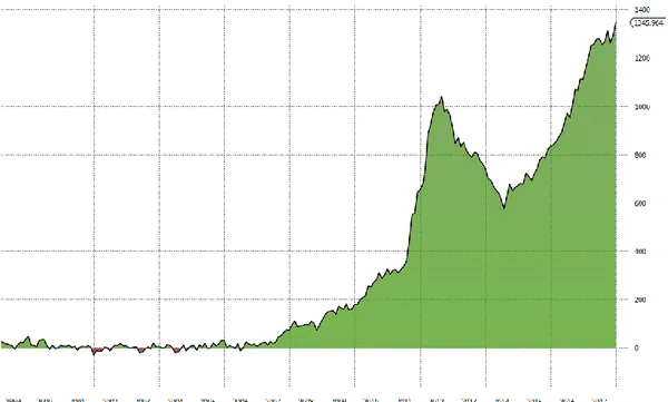
In order to conduct the empirical analysis we use daily premia for the sovereign Italian 10y CDS contracts and the BTP-Bund spreads6 (Di Cesare et al., 2013) for the interval 2007-20177 (respectively, 2522 observations). Data come from Bloomberg. Figure 1 reports the CDS and GBS (or commonly called “Spread”) series movement over the entire selected period.

6_{Bund yield has been selected as risk-free rate benchmark because this instrument has a similar}

liquidity level of BTP (Panzarino et al., 2016), it is a AAA rating instrument and it tends to outperform during periods of financial distress due to fly to quality phenomenon (Paret et al., 2019).

7_{The selected time horizon allows us not to include further exogenous events like US-China Trade}

War (2018-19) and Covid-19 Pandemic (2020) in order to emphasize the role of the European Central Bank (ECB) in affecting market interdependencies over time.

(5)

Figure 1: CDS spreads and GBS series (in %) from January 2007 to October 2017. Source: authors’ calculations in Eviews 10 based on Bloomberg data.

Time horizons selected to realize the whole analysis are not discretionary but justified by important historical events, as reported by Consob8_{, one of the most}

important Italian institutions. The dataset has been grouped in four distinct periods: • 2007-2010 (financial crisis);

• 2010-2012 (sovereign debt crisis);

• 2012-2014 (the years of liquidity drug - pre QE ); • 2014-2017 (the years of abundant liquidity drug - QE).

Table 1 reports the descriptive statistics of data for each sub period.

(6)

Table 1: Descriptive statistics of data from January 2007 to October 2017 (2522 Obs.)

Variable Average SD Min Max Median

10y CDS premia (basis points - 0.01% )

2007-10 47.86 40.11 8.21 163.55 33.82

2010-12 218.00 104.53 67.67 441.51 186.91

2012-14 173.59 44.26 97.84 262.91 169.89

2014-17 172.59 29.17 123.05 243.45 167.90

10y government bond yield spreads (%) 2007-10 0.6544 0.3962 0.1880 1.5860 0.5560 2010-12 2.6154 1.3509 0.6930 5.5250 2.0690 2012-14 2.1843 0.5755 1.1970 3.5090 2.2755 2014-17 1.4062 0.3027 0.8800 2.1300 1.3260

Source: authors’ calculations based on Bloomberg data.

The econometric model implemented is based on the methodology suggested by Gonzalo and Granger (1995). De Jong (2002) shows that, although Gonzalo-Granger and Hasbrouck approaches have their merits, the former is useful if one wants to construct the innovations in the efficient price from the full innovation vector (the major difference between the two approaches is the role of the variance of innovations). The analysis, therefore, develops in two stages.

In the first stage, we verify whether the short-term deviations of these two series converge towards the long-term equilibrium through a «cointegration analysis». The existence of a linear combination between these two series, indeed, supports the presence of a long-term equilibrium adjustment process, even if the series deviate one from the other in the short-term. In this case, series are cointegrated. In the second stage, by using the first stage results9_{, we will try to verify which}

market is able to embody more rapidly the risk information. In other terms, this allows us to evaluate the potential existence of a leader and follower market, as well as halfway situations. To do so, we set a bivariate Vector Error Correction Model (VECM), as suggested by Engle and Granger (1987).

9_{If the two series are not cointegrated then the VECM cannot be implemented because it is no more}

valid. In this case, we analyze the Granger-causality and the Impulse Responses by estimating an unrestricted VAR.

(7)

The formal specification of the model is defined by the following equations:

𝛥𝐶𝐷𝑆𝑡 = 𝛽10+ ∑𝑙𝑡=1𝛽1𝑡𝛥𝐶𝐷𝑆𝑡−1+ ∑𝑙𝑡=1𝛼1𝑡𝛥𝐺𝐵𝑆𝑡−1+ 𝜆1𝐸𝐶𝑇𝑡−1+ 𝜀1𝑡 (1)

𝛥𝐺𝐵𝑆_𝑡 = 𝛽₂₀+ ∑𝑙_𝑡=1𝛽_2𝑡𝛥𝐶𝐷𝑆_𝑡−1+ ∑𝑙_𝑡=1𝛼_2𝑡𝛥𝐺𝐵𝑆_𝑡−1+ 𝜆₂𝐸𝐶𝑇_𝑡−1+ 𝜀_2𝑡 (2) where:

• 𝛥𝐶𝐷𝑆_𝑡and 𝛥𝐺𝐵𝑆_𝑡 are, respectively, the first differences for the sovereign Italian 10y CDS spreads and the 10y government bond yield spreads series;

• β10 and β20 are, respectively, the constant terms of the equation (1) and (2); • 𝛥𝐶𝐷𝑆_𝑡−1and 𝛥𝐺𝐵𝑆_𝑡−1 are, respectively, the delayed first differences for

the sovereign Italian 10y CDS spreads and the 10y government bond yield spreads series;

• l is the number of lags;

• ECTt−1 is the Error Correction Term (ECT). It is defined as 𝐸𝐶𝑇_𝑡−1 =

𝐶𝐷𝑆_𝑡−1 − 𝛼 − 𝛾𝐺𝐵𝑆_𝑡−1. In simple terms, it measures the deviations between the CDS and GBS at time (t-1) with respect to the theoretical long period equilibrium. γ is the cointegrating coefficient and α is the intercept of the cointegrating term;

• λ1 and λ2 are the adjustment coefficients. They describe the speed of

adjustment back to the long period equilibrium, that is they measure the proportion of correction of the series deviations from the long-run relationship;

• ε1t and ε2t are, respectively, the error terms of the equation (1) and (2).

It is intuitive that, for the aim of the analysis, the evaluation of the sign10_{and the}

statistically significance of the adjustment coefficients (λ1 and λ2) allows us to know

which market contributes to the adjustment process toward the long period equilibrium and which market is able to embody more rapidly the credit risk information than the other one. Hence, I should distinguish four cases:

• if λ1 is statistically significant and negative then it implicitly means that the bond

market embodies more rapidly the credit risk information than the sovereign CDS market. This means that the sovereign CDS market is trying to restore the long-run equilibrium;

• if λ2 is statistically significant and positive then it implicitly means that the

sovereign CDS market embodies more rapidly the credit risk information than the bond market. This means that the bond market is trying to restore the long-run equilibrium;

• if λ1 is statistically significant and negative and λ2 is statistically significant and

positive then both markets contribute to the adjustment process towards the long-run equilibrium. In this case, by following Gonzalo-Granger (1995), in order to evaluate the effective contribution of each market in the adjustment

10_{We should expect the negative sign for λ}

1 and the positive sign for λ2 in order to favor the process

(8)

process, we follow the concept of Market Share (MS)11_{. According to how the}

MS formula has been defined, we distinguish between three sub cases:

a) if MS ≈ 1 then the sovereign CDS market is the leading market and the bond market is the lagging market;

b) if MS ≈ 0 then the bond market is the leading market and the sovereign CDS market is the lagging market;

c) if MS ≈ 0.5 then both market contribute in the same way;

• if only one of the adjustment coefficients is statistically significant and it present the correct sign then only that market contributes to the price discovery of the credit risk and to the adjustment process towards the equilibrium.

Given that the implementation of the just described model (bivariate VECM) requires that the two series are cointegrated, if this is not the case, then we set an unrestricted VAR to estimate the possible existence of a Granger-causality (unidirectional or bilateral) and, eventually, the Impulse Responses.

4. Main Results

In this section, results are discussed separately depending on the distinct stages of the crisis. All preliminary and complementary tests on time series are reported in the Appendix. Further statistical tests validating the acceptance of OLS assumptions are not reported here. With regard to these latter tests, they confirm the presence of heteroskedasticity, no serial correlation and non-normal distributed residuals. To limit the problem of the heteroskedasticity, we calculate robust estimates by using the Huber-White procedure. The normality assumption allows us to exact inference about the estimates and standard errors of the estimated coefficients. However, even when the normality assumption is not valid (but all the other assumptions are), the estimates are still consistent and the Central Limit Theorem allows making inferences that are valid in an asymptotic sense (Wooldridge, 2003). In the VAR model setup, in order to choose the optimal lag length, we follow the Hannan-Quinn criterion as suggested by Liew (2004)12.

4.1 Financial crisis: 2007-10

According to the first stage of the analysis, we evaluate the existence of cointegration between the two series through the Augmented Dickey-Fuller Test.

11_{The formula suggested by Gonzalo and Granger (1995 ) is the following:}_{𝑀𝑆 =} 𝜆2

𝜆2−𝜆1

12_{According to the author, the Hannan-Quinn criterion is the most efficient when observations are}

(9)

The latter is reported in Table 2.

Table 2: Augmented Dickey-Fuller Test (period 2007-10) Augmented Dickey-Fuller Test

Residuals

Period t-Statistic Prob.∗

2007-10 -4.183509 0.0049

Source: authors’ own calculations in Eviews 10 based on Bloomberg data.

As suggested by the test, the two series are cointegrated. Therefore, it is possible to realize the second stage of the analysis and estimate the VECM in order to assess which market contributes to the adjustment process toward the long-term equilibrium and which one is “the more efficient” in incorporating more rapidly the sovereign credit risk information. The VECM estimation outputs are reported in the following Table 3 and Table 4.

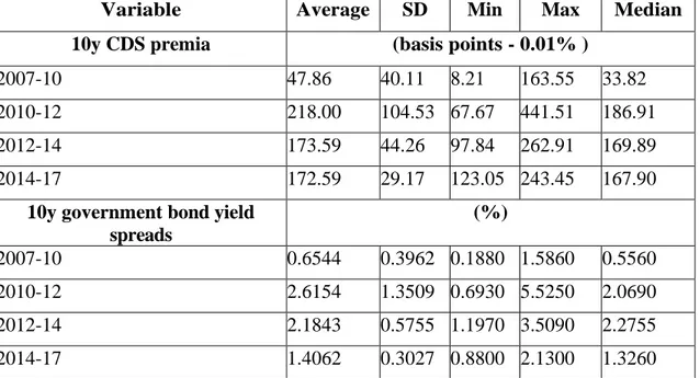
Table 3: VECM - dependent variable ΔCDS (period 2007-10) Coefficient Std. Error t-Statistic Prob.

β10 0.000749 0.001170 0.639985 0.5224 β11 0.063998 0.078157 0.818843 0.4132 β12 0.024382 0.071193 0.342479 0.7321 α₁₁ 0.165030∗∗∗ _0.059933 _2.753558 _0.0060 α₁₂ -0.017265 0.054450 -0.317088 0.7513 λ1 -0.003740 0.013030 -0.287049 0.7742

Note: *** signals parameter significance at 1%. Source: authors’ calculations in Eviews 10 based on Bloomberg data.

(10)

Table 4: VECM - dependent variable ΔGBS (period 2007-10) Coefficient Std. Error t-Statistic Prob.

β20 0.000613 0.001208 0.507348 0.6121 β21 0.062537 0.062073 1.007475 0.3141 β22 -0.069744 0.057683 -1.209103 0.2270 α21 0.236661∗∗∗ 0.054175 4.368449 0.0000 α22 -0.063678 0.055415 -1.149114 0.2509 λ2 0.051628∗∗∗ 0.012697 4.066062 0.0001

As we can see from Table 3 and Table 4, only λ2 is statistically significant and

positive while λ1 is negative but not statistically significant. This means that the

CDS market (lead) embodied more rapidly the credit risk information than the bond market (lag) during the financial crisis period and that this latter market moved in the direction to restore the long-run equilibrium relationship.

4.2 Sovereign debt crisis: 2010-12

We evaluate the existence of cointegration between the two series through the Augmented Dickey-Fuller Test. The latter test is reported in Table 5.

Residuals

2010-12 -5.011417 0.0002

Once again, the two series are cointegrated. The VECM estimation outputs, relative to this interval, are reported in the following Table 6 and Table 7.

(11)

Table 6: VECM - dependent variable ΔCDS (period 2010-12) Coefficient Std. Error t-Statistic Prob.

β₁₀ 0.002002 0.004302 0.465405 0.6418 β11 0.097455 0.088156 1.105493 0.2693 β12 -0.002739 0.067369 -0.040664 0.9676 α11 0.079697 0.079522 1.002194 0.3166 α12 -0.092484 0.064437 -1.435251 0.1516 λ1 −0.048971∗∗ 0.020721 -2.363368 0.0184

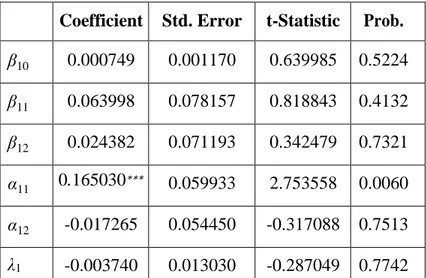
Table 7: VECM - dependent variable ΔGBS (period 2010-12) Coefficient Std. Error t-Statistic Prob.

β20 0.003343 0.004593 0.727878 0.4669 β21 0.166936∗∗∗ 0.061077 2.733217 0.0064 β22 0.024361 0.056063 0.434536 0.6640 α21 -0.028135 0.077136 -0.364747 0.7154 α22 −0.139668∗∗ 0.070373 -1.984683 0.0475 λ2 0.012396 0.022556 0.549555 0.5828

Table 6 and Table 7 show that only λ1 is statistically significant and negative while

λ2 is positive but not statistically significant. This means that the bond market (lead)

embodied more rapidly the credit risk information than the CDS market (lag) during the sovereign debt crisis period. The CDS market, therefore, favored the process of adjustment towards the long-run equilibrium relationship.

(12)

4.3 The years of liquidity drug - Pre QE: 2012-14

In the period immediately after the sovereign debt crisis, there is no cointegration between the series as supported by the Augmented Dickey-Fuller Test. The latter test is reported in Table 8.

Residuals

2012-14 -1.055049 0.9339

At this point of the analysis, given that there is no cointegration, we analyze the Granger-causality between the CDS and GBS series in order to see if one time series is useful in forecasting another one. Naturally, the Granger-causality is not necessarily “true causality”, econometricians assert that the Granger test finds only "predictive causality" (Diebold, 2001). Table 9 reports the outcomes of the causality test.

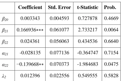
Table 9: Granger-causality Test (period 2012-14)

Null Hypothesis Obs. F-Statistic Prob.

GBS does not Granger-Cause CDS

480

22.5738 0.0000 CDS does not Granger-Cause GBS 1.09709 0.3347 Source: authors’ own calculations in Eviews 10 based on Bloomberg data.

Table 9 shows that GBS Granger-causes CDS premia but not the other way round (unidirectional Granger-causality). Therefore, it can be interesting to estimate the reaction of the CDS premia in response to the shocks of the GBS variable. In particular, a unit shock is applied to the error of the latter. Figure 2 shows the responsiveness of the CDSs to a unit shock of GBS variable.

(13)

Figure 2: Unit Shock Impulse Response (period 2012-14). X-axis in days. Y-axis in percentage points. Source: authors’ own calculations in Eviews 10

based on Bloomberg data.

As it is possible to note, after a unit shock in the GBS variable, the CDS spread tends to increase in the next day after the shock and it tends to stabilize starting from the next second day.

4.4 The years of abundant liquidity drug - QE: 2014-17

As well as the period 2012-14, during the period 2014-17 there is no cointegration between the series as supported by the Augmented Dickey-Fuller Test reported in Table 10.

Residuals

2014-17 -2.298192 0.4338

(14)

Also in this case, since there is no cointegration in the current sub period, we check for the Granger-causality between the CDS and GBS series. Table 11 reports the outcomes of the causality test.

Table 11: Granger-causality Test (period 2014-17)

Null Hypothesis Obs. F-Statistic Prob.

GBS does not Granger-Cause CDS

580

12.8949 0.0000 CDS does not Granger-Cause GBS 0.60355 0.6129 Source: authors’ own calculations in Eviews 10 based on Bloomberg data.

Table 11 shows, once again, the unidirectional Granger-causality running from the GBS to CDS premia. Figure 3 shows, therefore, the CDSs’ Impulse Response.

Figure 3: Unit Shock Impulse Response (period 2014-17). X-axis in days. Y-axis in percentage points. Source: authors’ own calculations in Eviews 10

based on Bloomberg data.

After a unit shock in the GBS variable, the CDS spread tends to increase up to the next third day after the shock and it tends to stabilize starting from the next fourth day.

(15)

5. Economic Discussion

In order to explain in detail the above results it is necessary to call to mind the ECB monetary policy during this time of crisis. One of the first effects of the financial crisis, recognized in Europe since mid-2008, was the breakdown of trust among banks and, in turn, of the interbank market.13 By observing Figure 1, we can note the first relative maximum for both series, the first real signal of the evident ongoing economic difficulties. The breakup of the interbank market in Europe caused an immediate general increase in the interbank interest rates level and, as consequence, in the interest rates level to retail customers during the period 2008-09. The necessity of liquidity for the banking system determined, on one side, the massive sales of their assets by banks and, on the other side, the famous “credit crunch” towards the real economy. During this period of lack of liquidity (from mid-2008 up to the end of 2009), the traditional transmission mechanism of the ECB monetary policy was literally unable to operate. The ECB, therefore, introduced the so-called “unconventional” policy measures (in particular, the Enhanced Credit Support14_{) in}

addition to the simultaneous gradual reduction of the policy interest rate level (which fell from 4.25% in October 2008 to 1% in May 2009). The results of the previous analysis, for the period 2007-09, show that when the banking system was not yet much affected by an enormous amount of liquidity in circulation, the CDS market has been able to embed more rapidly than the bond market the information on the augmented level of sovereign credit risk. This result confirm its superior capacity in the credit risk price discovery process in a situation of normal (more precisely, “partial”) functioning of the financial markets. The augmented sovereign credit risk level caused by the banking system trouble depends on the existence of a close relationship (“doom loop”) between State and banking sector. In other terms, the application of the bailout principle determines the transfer of risk from the latter to the former. At the same time, however, national banks play a fundamental role in the purchase of the national bonds, definitely much more than foreign banks. The period directly following (2010-12) was very delicate for the Eurozone in general (let us remember the famous Greek crisis between 2009 and 2010), but in particular for Italy. This period is also known as the “years of sovereign debt crisis” in the Eurozone.15_{However, this historical time interval was very relevant for the}

Italian economy. In the summer of the 2011, indeed, the so-called "spread crisis" exploded (in this context, the term "spread" refers to the differential between the

13_{The breakup of trust can be traced back to the famous American subprime mortgage crisis}

exploded in 2007.

14_{The ECB did unconventional measures by means of which it increased the maturity of the main}

refinancing operations (MROs) from 3 months to 1 year (LTRO) providing all the liquidity required by banks at a fixed rate (fixed rate full allotment system). It amplified the eligibility of bonds accepted as collateral and purchased covered bonds (60 billion in 2009 and 40 billion in 2011).

15_{In Greece, the problem was the massive public debt; for other countries, especially Spain and}

Ireland, the problem was the bank debt successively translated in public debt because of the State aids.

(16)

10-year BTP yield and that of the 10-year Bund) and hit the country of Italy.16_The

fundamental aspect that should be noted is that the risk associated with the spread level is not a pure credit risk (as measured by the hazard rate level of the CDS instrument), but it is also a measure of debt redenomination risk, that is the risk that Euro Area sovereign debt could be redenominated into new local currencies. Nevertheless, in November 2011 the high spread level was perceived as a probable Italian default (the spread comes to touch the historical record of 574 basis points!).17_{A situation of reversal capital flow was easily predictable because}

almost half of the Italian public debt was in foreign hands. Italian banks, moreover, were having trouble raising funds on institutional markets because of spread crisis and they tried to collect capital mainly from retail customers. At that time, the real problem was the need for liquidity; it was not a solvency problem, even though the bond market was very thin. Although the higher Italian sovereign risk was captured by the increasing Italian sovereign CDS spreads, the attention of financial investors and foreign governments remained the bond spread level. Reported results for the period 2010-12, indeed, show that the bond market (lead) embodied more rapidly the credit risk information than the CDS market (lag) and that the latter moved in the direction to restore the long-run equilibrium relationship. Why do we obtain this result? In that period, the CDS market stopped working: the trade levels were extremely limited (almost non-existent) because of the scarcity of investors to incur the counterparty risk as well as the illiquidity of this instrument. As a result, the CDS market was no longer a reliable indicator of sovereign credit risk. Given that the true point was the necessity of liquidity for Italy (and Spain), in order to avoid the Euro breakup, the ECB launched the VLTRO (Very Long Term Refinancing Operation - 3 years LTRO) in December 2011.18_{Through this measure, at the rate}

of 1% (indexed to the MRO rate), the ECB made available more than one trillion of euros to the banking system (Cesaratto, 2016). Naturally, this was particularly beneficial for Italian and Spanish banks that had the possibility to use this liquidity to satisfy their operational requirements and allow the rollover of the national public debt. It is clear that this was for the ECB a way to finance indirectly the public debt

16_{In May of the same year, S&P revised the outlook on Italy from “stable” to “negative”. When the}

1st July was diffused the S&P’s bulletin that evaluated the public deficit (and debt) reduction plan drawn by Berlusconi’s government (May 2008 - November 2011), the negative advice had an immediate dramatic effect on the Bund spread that expanded radically. On 7 July, the BTP-Bund spread soared beyond the quota 226 basis points, the record from the birth of the Euro. After that day, new records have been recorded. The BTP-Bund spread stabilized in August, but in September, when the S&P rating agency announced the downgrade of Italy, both CDS spread and bond spread sharply increased. The entire Europe (especially France and Germany) focused on the Italian government measures on debt and growth.

17_{On 9 November, Berlusconi’s government fell down and the President of the Italian Republic}

(Napolitano), on 16 November, instructed Mario Monti to constitute a new technical government. Europe reacted positively to that guards change. Indeed, the spread went down at 368 basis points on 6 December. However, it went up again at 500 basis points in the end of the year.

18_{In 2009, the ECB launched a LTRO (1 year). However, the VLTRO represented a more powerful}

(17)

of member States without negating the rules of its Statute. A pure consequence of this and all the other measures realized by the ECB in order to provide liquidity for the banking system have enforced the strict relationship between national banks and States.19 The GBS became the observed indicator (by traders) of the sovereign risk. The abundant liquidity of bonds made these instruments much more tradable than others. Therefore, the spread level affected by strong selling and buying, started to be a good indicator of the market sentiment on the sovereign credit risk. The events of July 2012 were definitive confirmation. Despite the tough reforms undertaken by Monti’s government (especially the pension reform or Fornero reform), in July the spread had returned to the levels it had touched before the fall of the Berlusconi’s government, more than 500 basis points. At a speech in London on 26 July 2012, the ECB President gave an account of the Eurozone economy. Bond yields of weak euro-member Governments were soaring, and traders doubted that national, Euro or EU level institutions could act together in time to avert disaster. The ECB President Mario Draghi tried to convince international investors that that the region’s economy was not as bad as it seemed. Then he made a momentous remark: «Within our mandate, the ECB is ready to do whatever it takes to preserve the Euro. And believe me, it will be enough». Traders reacted immediately to Draghi’s forthright resolution, and a week after his speech the ECB announced a program to buy the bonds of its distressed countries, known as Outright Monetary Transactions. Although the ECB never ended up using this program, the promise was enough to calm investors and bring down bond yields across the Eurozone (Nelson, 2017). The explicit introduction of the forward guidance by the ECB has been fundamental in order to reduce the gap within the BTP-Bund yield spread on which was concentrated the attention for the sovereign risk appraisal by international investors and save the whole Eurozone (not only Italy). In line with this argumentation, the analysis shows that the bond market (lead) embodied more rapidly the credit risk information than the CDS market (lag) during the sovereign debt crisis period (2010-12). This outcome would seem to support the idea that, in situations in which all financial investors go searching liquid assets, the CDS market (an illiquid market by nature) lose a fundamental part of its information power and the bond market (a very liquid market) starts to become the key market in the discovery process of the sovereign credit risk.

What happened when the system started to be fully flooded of liquidity?

On 6 September 2012, the ECB announced the potential revival of purchases of public securities already carried out in 2010 and in 2011 with the Security Market Program (SMP)20, but this time on a scale potentially unlimited, that is the Outright Monetary Transactions (OMT) or “Big Bazooka”. The OMT was certainly effective in reducing the long-term interest rates for Spain and Italy to more sustainable levels and in encouraging the recovery of interbank loans and the early

19_{It should be not a surprise that, to this day, around 2/3 of the Italian public debt is held by residents:}

Bank of Italy, national banks, insurance companies, institutional funds and retail (Bini et al., 2018).

(18)

repayment of VLTRO funds during the period 2013-14. Moreover, also the Target 2 balances was reduced (Cesaratto, 2016), as reported in the Figure 4.

Figure 4: Target 2 Net Claims differential between Germany and Italy (in millions) from 1999 to 2018. Source: Bloomberg.

This measure was fundamental in order to stabilize markets and convince the financial operators that it would not have been worthwhile (for them) to move against the ECB policy. Naturally, the amount of (low-cost21) liquidity provided by the Central Bank has been enough both to stimulate the revival of trust in the interbank market and to allow banks to realize genuine free lunches (or arbitrages) by investing in government bonds. CDSs, in a system that already recorded high amount of outstanding cash, was no longer considered as benchmark of the sovereign credit risk: the level of trades were sporadic because of the increased counterparty risk perceived by operators that continued to prefer liquid instruments. The whole attention of the financial world was completely focused on the bond market, where the flight-to-quality strategy represented the main allocation strategy for fixed income portfolio managers and defensive hedge funds. For the period 2012-14, the two examined series are not cointegrated. The Granger-causality test, however, shows that the bond spreads Granger-caused the CDS premia during this market phase.

What should we expect for the interval 2014-17 when the ECB increases the “liquidity drug” in the financial markets with the Quantitative Easing (QE)?

(19)

The increased pace of the expansive ECB monetary policy starting from the 2014 was related to the fear of deflation. This latter would have surely weakened the fragile structure of the peripheral countries heavily indebted (as Italy). In absence of a limited fiscal policy (due to “austerity”), the monetary policy is the only tool able to stimulate a potential up trend of the national income level (Blanchard et al., 2009). The Central bank policy, however, is only able to act on the short-term rates while some households’ consumption decisions are affected by the long-term rates. For ease of reference, let us assume that long-term rates are the sum of two components, the short-term rates and a risk premium component. The core problem is that, in a climate of difficulties in the real economy, the long-term rates, even operating a short-term rates reduction, tend to increase due to the increased risk component. This condition is further aggravated in a situation of zero lower bound. How can this limit be overcome? Once again, the Holy Grail is the cost-free and massive liquidity provision to the economic system! The spectrum of deflation and the necessity to avoid that European unemployment became structural were sufficient to incentivize the ECB to continue in this direction. The ECB, in June 2014, announced the TLTRO (Targeted Long Term Refinancing Operation), preferential lending to banks (with expiry date four years for banks that respect the ECB rules) but linked to the amount of loans that credit institutions in turn provide to businesses in order to sustain the real economy. As already mentioned, in September of the same year, the policy rate level went down at the 0.05% and the ECB Governor Draghi officially adopted the so-called “forward guidance” stating that that level would have been maintained “low” for a long time. This measure was adopted in order to correct what market was discounting in terms of its expectation on long-term interest rates. Moreover, during this period, the Central Bank realized also the purchase program of covered bonds and Asset-Backed Securities (ABS). Nonetheless, these measures were not sufficient to reduce the high-risk premium. What did the ECB think to do in order to renormalize markets? In January 2015, Draghi announced the Quantitative Easing (QE). In March of the same year, indeed, the ECB implemented the large-scale purchase program of 60 billion of euros (monthly) of government bonds, covered bonds and ABS based on specific rules22. The deadline of this exceptional and unconventional measure had programmed in September 2016. How did market react? The equity market prices reacted positively (merely as example, let us imagine the possibility for firms to low cost finance their stock buybacks!), the Euro-Dollar exchange rate depreciated and the bond spread decreased. Markets were already enormously drugged of outstanding liquidity but the ECB continued its expansive monetary policy in the course of 2016 and 2017. In particular, on 10 March 2016, the Central Bank reduced the policy rate to 0.00%

22_{The purchase of government bonds by the ECB in the secondary market was to be carried out}

according to a risk-sharing criterion with national Central Banks. In particular, only 20% of the risk was to be borne by the ECB. In addition, the ECB had a "double limit": one of 33% in relation with the public debt of each issuer and another of 25% for each issue. The maturity of the bonds to be bought varied from 2 to 30 years, therefore, short, medium and long-term bonds.

(20)

and the TLTRO II was announced, leaving his purchase program unvaried.

Once again, as for the previous period 2012-14, during the interval 2014-17, when financial markets were fully plenty of liquidity, the two examined series continued to be not cointegrated. The Granger-causality test show that the bond spreads Granger-caused the CDS premia. This would prove that, in abnormal (drugged) market conditions, the natural connection between the CDS market and bond market tend to be obfuscate and the price discovery process of credit risk altered. In a similar backdrop, operators focus predominantly on current market topics (what the whole market is looking at that particular moment) and specialized financial instruments, as CDSs, can lose their core function in the price discovery process of risks due to the undermined CDS market liquidity. This condition, by the way, is even more valid inside a global market in which almost the 70% of trading activity takes place by means of algorithms.

6. Conclusions

In order to analyze the lead-lag relationships between Sovereign Credit Default Swap (CDS) premia and government bond yield spreads (GBS), we employed 2522 daily observations of Italy 10 years CDS premia and BTP-Bund spread values from January 2007 to October 2017, provided by Bloomberg. This study concludes that, in normal market conditions, the CDS is the best instrument in the price discovery process of the credit risk. During the financial crisis (2007-10), when markets lacked liquidity, the CDS market leads the bond market to incorporate more rapidly the sovereign credit risk information. In the following period, when markets started to be affected by the expansive ECB monetary policy albeit maintaining part of their normal structure, this relationship reverses. In fact, during the sovereign debt crisis (2010-12), the bond market leads the CDS market to incorporate more rapidly the sovereign credit risk information. The most impressive result is that, in the sub periods in which the market functioning comes completely altered by the excessive outstanding liquidity (2012-14 and 2014-17), because of the unconventional measures undertaken by the ECB, the two series are no more cointegrated. In particular, during the years of the liquidity drug - pre QE (2012-14), the GBS Granger-cause the CDS spreads. This last result is further confirmed during the years of abundant liquidity drug - QE (2014-17).

(21)

References

[1] Amadei, L., Di Rocco, S., Gentile, M., Grasso, R. and Siciliano, G. (2011). Credit Default Swaps: Contract Characteristics and Interrelations with the Bond Market. SSRN Electronic Journal.

[2] Bai, J. and Collin-Dufresne, P. (2011). The CDS-Bond Basis During the Financial Crisis of 2007-2009. Working Paper.

[3] Bini, F. and Ricciardi, R. (2018). Chi ha in mano il debito pubblico italiano: l'evoluzione in 30 anni. [Online] La Repubblica. Available at: <https://www.repubblica.it/economia/2018/05/29/news/chi_detiene_il_debito _pubblico_italiano_30_anni_di_cambiamenti-197562983/> (accessed 7 November 2020).

[4] Blanchard, O., Amighini, A. and Giavazzi, F. (2009). Macroeconomia. Il Mulino.

[5] Cesaratto, S. (2016). Sei lezioni di economia. Reggio Emilia: Imprimatur. [6] Coudert, V. and Gex, M. (2010). Credit Default Swap And Bond Markets:

Which Leads The Other?. [Online] Core.ac.uk. Available at: https://core.ac.uk/download/pdf/6612165.pdf (accessed 8 December 2020). [7] De Pooter, M., Martin, R. F. and Pruitt, S. (2018). The Liquidity Effects of

Official Bond Market Intervention. Journal of Financial and Quantitative Analysis, 53(01), pp.243-268.

[8] De de Jong, F. (2002). Measures of contributions to price discovery: a comparison. Journal of Financial Markets, 5(3), 323-327.

[9] Di Cesare, A., Grande, G., Manna, M. and Taboga, M. (2013). Recent estimates of sovereign risk premia for euro-area countries. Banca d'Italia. Available at:

https://www.bancaditalia.it/pubblicazioni/altri-atti-convegni/2013-2-sovereign-debt-crisis/dicesare.pdf (accessed 8 December 2020).

[10] Diebold, F. X. (2001). Elements of Forecasting (2nd ed.). Cincinnati: South Western.

[11] Duffie, D. (1999). Credit Swap Valuation. Financial Analysts Journal, 55(1), pp.73-87.

[12] Elton, E., Gruber, M., Agrawal, D. and Mann, C. (2002). Explaining the rate spread on corporate bonds, Journal of Finance 56, 247-277.

[13] Engle, R. F. and Granger, C. W. J. (1987). Co-Integration and Error Correction: Representation, Estimation, and Testing. Econometrica, 55(2), p.251.

[14] Fontana, A. and Scheicher, M. (2016). An analysis of Euro Area sovereign CDS and their relation with government bonds. Journal of Banking & Finance, 62, pp.126-140.

[15] Gonzalo, J. and Granger, C. (1995). Estimation of Common Long-Memory Components in Cointegrated Systems. Journal of Business & Economic Statistics, 13(1), pp.27-35.

(22)

[16] Gyntelberg, J., Hördahl, P., Ters, K. and Urban, J. (2016). Arbitrage Costs and the Persistent Non-Zero CDS-Bond Basis: Evidence from Intraday Euro Area Sovereign Debt Markets. SSRN Electronic Journal.

[17] Koutmos, D. (2018). Interdependencies between CDS spreads in the European Union: Is Greece the black sheep or black swan? Annals of Operations Research.

[18] Lehmann B. N. (2004). Some desiderata for the measurement of price discovery across markets. Journal of financial markets.

[19] Liew, V. K., (2004). What lag selection criteria should we employ? Economics Bulletin, 33(3), pp. 1-9.

[20] Longo, M. (2018). Quali rischi corrono davvero le banche se lo spread va a 400. [Online] Ilsole24ore.com. Available at:

<https://www.ilsole24ore.com/art/quali-rischi-corrono-davvero-banche-se-spread-va-400-AEOZejUG> (accessed 7 November 2020).

[21] Ministero dell'Economia e delle Finanze (MEF), 2017. The Secondary Market For Italian Government Securities. [Pdf] Washington DC: Ministero dell'Economia e delle Finanze. Available at:

<http://pubdocs.worldbank.org/en/625091493405007505/bonds-conf-2017-Davide-WB-conference-Italy-experience-on-ETPs.pdf> (accessed 4 October 2020).

[22] Nelson, E. (2017). Five years ago today, Mario Draghi saved the Euro. [Online] Quartz. Available at: https://qz.com/1038954/whatever-it-takes-five-years-ago-today-mario-draghi-saved-the-euro-with-a- momentous-speech/ (accessed 26 July 2017).

[23] Palladini, G. and Portes, R. (2011). Sovereign CDS and Bond Pricing Dynamics in the Euro-Area. NBER Working Paper Series.

[24] Panzarino, O., Potente, F. and Puorro, A. (2016). BTP Futures and Cash Relationships: A High Frequency Data Analysis. SSRN Electronic Journal. [25] Paret, A.C. and Weber, A. (2019). German Bond Yields and Debt Supply: Is

There a "Bund Premium"? IMF Working Papers.

[26] Wooldridge, J. M. (2003). Introductory econometrics. Mason, Ohio: Thomson/South-Western.

(23)

Appendix

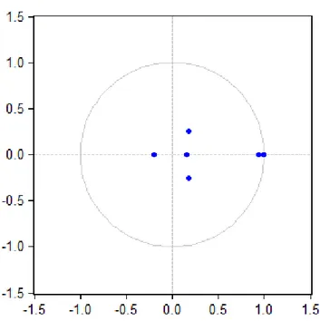
Table 12: Lag Order Selection Criteria

Period Lag Hannan-Quinn Information Criterion

2007-10 2 −8.133452∗

2010-12 2 3.324475∗

2012-14 2 −5.628491∗

2014-17 3 −6.027153∗

*indicates lag order selected by the criterion. Source: author’s own calculations in Eviews 10

Figure 5: Inverse Roots of AR Characteristic Polynomial (period 2007-10). Source: authors’ own calculations in Eviews 10 based on Bloomberg data.

(24)

(25)