Università degli Studi di Siena
DIPARTIMENTO DI ECONOMIA POLITICA
Mauro Caminati
Complementary, Opportunity
and The Co - Evolution of Techniques
1. Introduction
The literature on technological innovation has emphasised two related points concerning the changing degree of input complementarity throughout the life cycle of a technology1. (i) There is a natural tendency throughout the life cycle of a given technology or process towards an increasing complementarity of its components. This tendency is spurred by the selective pressure towards tight integration of the process elements regarded as a ‘natural’ condition enabling the elimination of ‘slack’. (ii) The initial non-integrated regime lends itself to easy adaptation of its components (is ‘fluid’), while the later highly integrated regime is more rigid. The selective pressure towards tight integration is therefore weak, as long as processes face a turbulent environment. The transition between the two regimes is marked by the emergence of a dominant configuration of the new technology.
A reason behind point (ii) is that the adaptation of a non-interrelated process is likely to face lower adjustment costs2. Hence, the conclusion that the rigid regime can not set in before the environment becomes relatively stationary. What is left unexplained by the argument above is the role, if any, of complementarity, in the transition between the two regimes, hence in the emergence of a dominant technological solution.
1 “Early in the life of process and product...the process itself is composed largely of unstandardized and manual
operations, or operations that rely on general-purpose equipment. During this state, the process is fluid , with loose and unsettled relationships between process elements. Such a system is ‘organic’ and responds easily to environmental change, but necessarily has ‘slack’ and is ‘inefficient’.
As an industry and its product group mature, price competition becomes more intense. Production systems, designed increasingly for efficiency, become mechanistic and rigid. Tasks become more specialized and are subject to more formal operating controls. In terms of process, the production system tends to become more elaborated and tightly integrated through automation and process control. Some subprocesses may be highly automated with process-specific technology while others may still be essentially manual or rely upon general-purpose equipment. As a result, production process in this state will have a segmented quality. Such extensive development can not occur however until a product group is mature enough to have sufficient sales volume and at least a few stable product designs.
As a process becomes more highly developed and integrated and as investment in it becomes large, selective improvement of process elements becomes increasingly more difficult. The process becomes so well integrated that changes become very costly, because even a minor change may require changes in other elements of the process and in the product design. Process redesign typically comes more slowly at this stage, but it may be spurred by the
development of a new technology or by a sudden or cumulative shift in the requirements of the market. If changes are resisted as process technology and the market continue to evolve, then the stage is set for either economic decay or a revolutionary as opposed to evolutionary change.” (Utterback and Abernathy [1975], pp. 426-7).
2 Suppose we fix a strength of adjustment costs through the cost required, on average, by a ‘unit-step’ away from a
technical position, that is, by the re-configuration of a unit component of that position. For a given strength of
adjustment costs, the adaptation of a non-interrelated process is less expensive, because it involves, on average, the re-configuration of a lower number of components. Hence, for the given structure of adjustment costs, non-interrelated processes are also more flexible, in the sense of Marschack and Nelson [1962]. However, modern multi-task equipment achieves flexibility through a different route; it reduces or eliminates the need of reconfiguration of a technical position in the face of a change in the environment. This is consistent with relatively high integration and complementarity constraints (cf. Milgrom and Roberts [1990]).
This paper argues that Stuart Kauffman’s work on co-evolution offers a candidate explanation of this point. For the sake of simplicity, we abstract completely from adjustment costs. It is shown how a varying degree of input complementarity across a set of competing technological orders within a radically new technology, is per se sufficient to afford a selective advantage to a subset of these orders, which are then more likely (ceteris paribus) to emerge as dominant. The process is best understood if the turbulence of the environment is considered as endogenous, rather than exogenous. This is not the case in the classic contribution by Utterback and Abernathy [1975], where the drive towards increasing integration and standardization of a process components is mainly regarded as a by-product of an unexplained tendency towards maturity (lower variation) within the product group, which justifies the focus on cost. Instead, in this paper the turbulence of the environment is precisely determined by the fact that the competition between the multiplicity of technical orders in the different sectors of activity is not at rest.3 The exclusive focus on complementarity and on broadly defined technological orders4 of a radically new technology with pervasive cross-sector effects distinguishes this paper from a recent literature on technological standards, which is otherwise quite close in spirit5.
The suggested explanation draws upon some “general rules of structure and change” of the type alluded to by Stephen Gould6. A system, biological, organizational or technological, composed of many heterogeneous units has a global performance operation depending both on the efficiency with which each component part performs its specific function, and on the way the single units interact. Integration between components can be defined to be more or less tight, depending on the average number of units affecting the performance operation of a single unit. If the units are not inter-related, (complementarity is low), a change improving the performance of a single component designed to serve a set of functions, does not conflict with the performance of other components,
3
Drawing the threads of various contributions, Anderson and Thusman [1990] add evidence from the U. S. flat-glass industry to point out that technological change follows a cyclical pattern consisting of “long periods of incremental change punctuated by technological discontinuities”. The discontinuity giving rise to the cycle is identified with a technological breakthrough.
“A revolutionary innovation is crude and experimental when introduced, but it ushers in an era of experimentation as organizations struggle to absorb (or destroy) the innovative technology. This era of ferment is characterized by two distinct selection processes: competition between technical regimes and competition within the new technical regime. This period of substantial product-class variation and, in turn, uncertainty ends with the emergence of a dominant design.” (Anderson and Thusman [1990], p. 615)
If competition between technical regimes is identified with the struggle between the ‘old’ and the ‘emerging’ technology, it is worth insisting that there may be radically different versions of the latter, identifying alternative technical orders. For this reason, the implications of competition within the new technical regime are far reaching. Such is the case, for instance, of the ‘battle’ between the direct-current and alternating-current systems in power generation (Hughes [1983], David [1992]).
4 See the historical example below in the text.
hence with the smooth operation of the process, resulting from the overall configuration of the system. In this case, evolution towards high levels of global performance can take place through a (possibly long) sequence of step-wise and relatively independent changes in the single units. The process of change is then ‘fluid’, and, “the system responds easily to environmental change”7 If, on the contrary, the system is composed of tightly inter-related units, the exploitation of the existing complementarities is an obstacle to the independent adaptation of the single units. In this sense, we can speak of complementarity constraints. Then, a state is soon reached in which every apparently-favourable change in a single component would conflict with the overall performance of the system. At this stage a relative stasis of change is observed; if change occurs at all, more than gradual, it is likely to be revolutionary, in that the simultaneous re-configuration of a large number of units is involved.
This type of argument has been explored in an abstract setting by Stuart Kauffman (Kauffman [1993]) through his model of an evolving string of N binary elements each functionally related to other K elements in the string. Kauffman’s N-K model is concerned with the evolution of a single string, and is intended as a fundamental, but preliminary building block towards the construction of more elaborate models with a view to suggest possible paths to self-organization in (biological) co-evolution. In the extended N-K model each string interacts with other strings: more specifically, every string element is related to C elements of every other interacting string. The relevance of Kauffman’s N-K model to the evolution of economic organizations has been pointed out in Westhoff, Yarbrough and Yarbrough [1996], Pagano [1998] and, more extensively, Levinthal [1997]. Whereas the above studies leave the problem of co-evolution mainly in the background, this is, instead, the main concern of this paper, which is also more directly focused on technological change. Here we hold to Mokyr’s analogy (Mokyr [1990], [1991]) between biological species and techniques. Moreover, if Kauffman’s work exploits to a large extent the simulation of large complex systems, we pursue as far as possible an analytical approach to the presentation of the main qualitative properties of the models.
As a matter of interpretation, to make our point sharper, we consider a process of technological co-evolution induced by one or more macroinventions (Mokyr [1990]). A macroinvention can be defined as breakthrough in scientific and or technological knowledge inducing a drastic and discontinuous re-orientation of technological opportunities across a large number of sectors. The re-orientation gives rise to a competition between alternative technological orders which may take place in the source sectors (those where the macroinventions originated), as
well as in the other sectors. It is a phase of substantial technological uncertainty, due to the fact that the new technological opportunities are still ill defined and may evolve rapidly. This phase ends with the emergence of a new set of inter-related dominant designs across sectors.
An example drawn from the history of electrification may serve to illustrate this point. As it has been recounted on many occasions, the electric-supply industry in its infant phase saw a fierce competition between the alternative technological orders represented by the direct current and alternating current systems. If the latter enjoyed generally lower long-distance transmission costs, one of its major drawbacks vis a vis the alternative system, till the late 1880’s, was the lack of an alternating current motor. The availability of a satisfactory direct current motor enabled instead the direct-current supply stations to “spread fixed generating costs by supplying electricity for power as well as for lighting” (David [1992], p.145). An alternating-current polyphase induction motor was patented by Nikola Tesla in May 1888 and marketed in 1992 by Westinghouse. As Devine [1983] puts it:
For the same output, a. c. [alternating current] motors were superior to d. c. [direct current] motors in a number of respects: they were smaller, lighter and simpler, did not spark, required very little attention and were quite a bit cheaper. But a. c. motors had one principal drawback: their speed could not be varied without seriously impairing performance. Frequency, not voltage, governs the speed of an induction motor, and it was not practical to provide variable-frequency current. (Devine [1983], p. 366)
If the relative diffusion of the a. c. induction motor, with respect to its competitor d. c. motor, was favoured by the growing availability of alternating current supplied by central power stations at relatively low transmission costs, the difficulties encountered in the speed variation of the former posed stronger complementarity constraints to a factory production system. These constraints did not prevent the a. c. induction motor to settle as the dominant technological solution in most production techniques. What took place was instead a co-evolution of designs towards a state such that they were simultaneously at, or close to, a ‘fitness peak’.
By 1901, many engineers felt that if efficient speed variation could be devised, the induction motor would be an important step toward the “ideal workshop”-a shop with a motor driving each tool or machine.
But during the first decade of the twentieth century, manufacturing methods began to call for more special-purpose machine tools, and these operated under comparatively narrow speed ranges... Of course, the availability of relatively cheap induction motors and the alternating current to run them were associated with this trend towards specialization. It is not clear whether increasing use of a.. c. motors was an important cause of specialization or a result of it. In either case, manufacturing’s need for speed variation that initially held back the spread of the a. c. motors diminished. (Devine [1983], pp. 366-67)
constraints within techniques and changing opportunities shaped by the interdependence relations across techniques. Moreover, the co-evolution framework exempts us from seeking unidirectional lines of causality, of the type alluded to by Devine.
In what follows, we attempt at showing how Kauffman’s work can be used to build a formal model of the phenomena outlined above. The chosen representation of technological co-evolution tends to emphasize how a technical change in one sector generates new and different technological opportunities (Nelson and Wolff [1997], Dosi [1997]) for other sectors. In other words, a step by a technical order on its fitness landscape8 can deform the fitness landscape of techniques referring to other sectors of activity. Here, the fitness landscape of a technical order is interpreted as the graph of a map associating every possible variant of the same order with its level of fitness, interpreted as a measure of performance in (adaptation to) the given environment. Technological opportunities act through birth and death of products, price effects and externalities.
If such interdependence effects are strong enough, the outcomes of technological evolution in any sector of activity are perturbed by the systematic deformation of the fitness landscape induced by the simultaneous evolution in the other sectors. In this scenario, complementarity constraints come to play a selective role because they affect the probability that technological systems are internally well adapted. This occurs because complementarity constraints, while restricting the set of profitable moves in technological space, increase the probability of evolution towards a stable design (in spite of the fact that the design may not be optimal ex-post), and give persistence to the technological opportunities across different sectors of activity. In this way, complementarity constraints contribute to reducing uncertainty and disorder within the technological system, regarded as a complex collection of evolving techniques.
For the sake of the argument, we shall assume that the available technical orders are uniformly distributed in K space, where K is a measure of input complementarity. Moreover, we shall assume away an ex-ante systematic relation between ‘integration’ and fitness contributions. It is as if every sample realization of a landscape is drawn from a distribution such that the degree of integration of a technical component is uncorrelated with its fitness contribution. As already anticipated, tighter integration brings in stronger complementarity constraints. On this premise, the fitness landscape of a more tightly integrated technical order is also more ragged, on average. Then, as revealed by Kauffman’s findings, on a more rugged landscape local optima are higher in number, although their average fitness value may be lower. Moreover, paths to local optima involve a lower number of steps.
These properties can be shown to imply that, at every stage in a process of technological co-evolution technical orders evolving on more rugged landscape have a higher probability of being simultaneously at a fitness peak, hence of evolving to a stable local optimum. If techniques have a sufficiently-large number N of components, there is a trade-off between the probability that a process co-evolves to a stable local peak and the average fitness value of a peak. Thus, it turns out that technical orders with an intermediate degree of integration enjoy a selective advantage over competitors characterized by very-high-or-low complementarity constraints. These properties hold true, no matter whether the routines driving technical evolution proceed by means of blind explorations (as mostly assumed by Kauffman), or through optimal choices within the local choice set. Any consideration of strategic rationality is assumed away.
As soon as technical orders in all (most) sectors are simultaneously at a fitness peak, co-evolution comes to a rest point (tends to be frozen). Hereafter, and up to the next macroinvention, technological evolution is mainly a matter of gradual adjustments within the orders that have been selected as dominant designs.
We may observe, in passing, how the emergence of technical orders well adapted to the given environment, does not rule out the selection of inferior local optima. This follows from the assumed lack of co-ordination between the local adaptations of the co-evolving techniques. Thus, there is scope for all sorts of path-dependence and irreversibility effects.
In part 2 we show how Kauffman’s N-K model provides a framework for the analysis of input complementarity in a process of technological exploration performed by one sector taken in isolation. Here we compare the properties of Kauffman’s blind-exploration and of an utterly intentional, deterministic dynamics. Coupled evolutions of many techniques simultaneously, are considered in part 3. They give rise to relations of interdependence across sectors. Here our formalization of the problem, although clearly inspired by Kauffman’s N-K-S-C model, departs in some respects from it. This enables us to support the main conclusions through analytic arguments. A study of the selective role of complementarity in a simulation experiment of coevolution completes our analysis. Section 4 draws the main implications of this line of research on the themes of technological evolution and productivity growth. It is argued that the model contributes to explaining the productivity slow-down during the transition between technological regimes.
2. Technological exploration and input complementarity
2.1
Let us think of a ‘method’ ai(t) in sector of activity i at time t as an historically contingent way of doing things as it applies to that sector of activity. Information on a given method is coded in a number of binary components or ‘traits’, each of which can assume the value 0 or 19. We may think of the string as a way of coding a specific combination of basic ideas. At each stage of technological exploration a method of production consists of the combination of a finite number of ideas, but the number of potentially accessible combinations tends to grow over time and the string length with it. To stress that the suggested explanation has little to do with the expanding dimension of the technological space, we shall assume, however, that the length of all strings is finite and fixed.
The higher or lower capacity of a method to gain and maintain widespread adoption within its sector of activity defines its competitive strength, or fitness, vis a vis the other methods potentially available for the same sector. As the remark on technological and price uncertainty illustrates, production cost at current prices is a determinant, but not the exclusive or even fundamental determinant of fitness.
There are S sectors in the economy. A method for sector i (i = 1, ..., S) is a string of N binary elements (xi1, xi2, ..., xiN), where each xij , j = 1, ..., N can assume value 0 or 1. There are then 2N possible methods for sector i, corresponding to the number of different states in the space {0, 1}N; they define the set Ai. We assume for simplicity that at any given date only one method is in use within each sector. A technical state of sector i is defined by a method in use in i.
Let xi and x’i be N-strings in Ai. The distance between xi and x’i is defined by the number of components of the former having a different value with respect to the corresponding components of the latter. More formally,
d(xi , x’i) = j=
∑
1 N (xij− x’ij)2The neighbourhood of xi is the set of strings in Ai with distance from xi less than or equal to 1. It consists of xi and its N neighbours.
9For the time being we abstract from the otherwise important distinction between information and knowledge and the
The fitness function of sector i is the map Vi : Ai → ℜ associating each method of sector i with its fitness value (a real number). In particular, the fitness value of a string results from the sum of the fitness contributions of its N components. More formally, the map Vi is defined as:
Vi(xi1, xi2, ..., xiN) = j=
∑
1 N Vij(xi1, xi2, ..., xiN)where Vij(xi1, xi2, ..., xiN) is the fitness contribution of the string component xij, given its configuration (xij = 0 or 1). For the present purposes Vij is best treated as a random real in the unit interval. The above notation attempts at formalizing the notion of input complementarity, in that, the fitness contribution of xij may depend not only on the configuration of this component, but also on the configuration of other string components. Kij ≤ N − 1 is the number of string components which are complementary with respect to xij; then, Kij + 1 is the number of non-redundant arguments of Vij(xi1, xi2, ..., xiN). For the sake of simplicity it is assumed that Kij is constant across components and across sectors:
Kij = K , j = 1, ..., N i = 1, ..., S
In the absence of complementarity (K = 0), Vij(xi1, xi2, ..., xiN) can be written as Vij(xij), and Vi(xi1, xi2, ..., xiN) =
j=
∑
1 N
Vij(xij). The highest-fitness method in Ai is then identified by the string such that the configuration of each component xij maximizes the fitness contribution Vij(xij) of that component.
The fitness landscape of sector i is the graph of Vi( ) on Ai.
A path in Ai joining xi to x’i is a sequence of strings in Ai such that xi and x’i are the first and last element in the sequence, respectively, and the distance between every couple of contiguous elements in the sequence is d = 1. A path joining xi to x’i is minimal if the distance from x’i is strictly decreasing along this path.
x’i is a local maximum of Vi(xi1, xi2, ..., xiN) on Ai if and only if on every path in Ai joining x’i to a string yi such that Vi(yi) > Vi(x’i) there is y’i such that Vi(y’i) < Vi(x’i) and d(x’i , y’i) < d(x’i , yi).
x’i is an isolated local maximum of Vi(xi1, xi2, ..., xiN) on Ai if and only if every neighbour xi of x’i satisfies: Vi(xi) < Vi(x’i). In what follows, we shall refer equivalently to isolated local maxima of Vi( ) on Ai, or isolated local peaks of the fitness landscape of sector i.
With reference to the case of zero complementarity, it is worth recalling how a change 0 → 1, or vice versa, in the configuration of a single string component, does not affect the fitness contribution of the other components. This simple fact confers striking properties to the K = 0 fitness landscape.
Proposition 1. Assume K = 0. If xi is a global maximum of Vi( ) on Ai, and yi an arbitrary string in this set, then Vi() does not decrease on every minimal path joining yi to xi.
The proposition is self evident. Since the path is minimal, there must be as many steps along the path as there are components of yi differing (in their configuration) from the corresponding components of xi. At every step along the path the distance from xi decreases, that is , there is another component of yi assuming the same value of the corresponding component of xi. This value maximizes the fitness contribution of the component (because xi is a global maximum) without decreasing the fitness contribution of the other components (because K = 0).
Proposition 2. If K = 0, the fitness landscape of sector i has at most one isolated local peak and a local maximum of Vi( ) on Ai is a global maximum (cf. appendix).
Remark 2.1: The probability that a randomly chosen state of a K = 0 landscape is a local peak is 1/2N. Let V*(N, K) be the expected fitness of a local peak on a N-K landscape. V*(N, 0) is independent of N and can be expressed as
E[ j N =
∑
1 Max(aj,bj)] = 0.666where (aj,bj) are N coulples of real random numbers uniformly distributed on the unit interval.
When K > 0, the choice of configuration maximizing the fitness contribution of the string component xij , given the configuration of the other N-1 sting components, may not positively contribute to the overall fitness of the method in use in sector i. The reason is that complementarity implies the possibility of a feed-back of uncertain sign from the new configuration of the component xij to the fitness contributions of the other components. A straightforward consequence of K > 0 is that fitness may decrease, locally, on a minimal path to a global optimum, because there may be situations where a fitness increment can be reached only through a changed configuration of two or more string components, simultaneously. This amount to the possibility of multiple isolated local optima. The situation is illustrated in fig.1, referring to the simple case N = 2 and K = 1.
(0,1)° • (1,1)
(0,0)• ° (1,0)
fig. 1
In this example, the set Ai of possible methods for sector i consists of four strings. The strings (0,0) and (1,1)
are isolated local peaks (black spots). The paths connecting the strings are made-up of contiguous sides of the square, but not of its diagonals, because diagonal steps involve the simultaneous change of more than one string-component. Fitness does not behave monotonically on every path joining (0,0) and (1,1).
When complementarity is maximal (K = N − 1) the fitness landscape is random, in the sense that the fitness values of neighbouring states are totally uncorrelated. A change (from 0 to 1, or vice versa) in the configuration of a single component, say component j of method i, assigns not only a new random fitness contribution to Vji, but also a new random contribution Vhi to every component h (h = 1, ..., N). The reason is, of course, that now xji is a non-redundant argument of Vhi (h = 1,...,N). Among the statistical properties of the K = N − 1 random landscape described in Kauffman [1993] , we stress the following:
Remark 2.2: Since the fitness value of every state on a K = N − 1 landscape is a random number, uniformly distributed between zero and one, the probability that a randomly chosen state of the lanscape is a local peak, i. e. is fitter than its N neighbours, is 1/(N + 1). Thus, there are on average 2N/(N + 1) local peaks on a K = N − 1 landscape.
Here is the main result of part 2. Proposition 3:
(i) Remark 2.1 implies V*(1, 0) = 0.666.
(ii) As N increases above 1, V*(N, N − 1) first grows above 0.666 and then decreases monotonocally to 0.5.
(iii) Let K = N − 1. Then V*(mN, K) = V*(N, K) for any m ≥ 1. Proof: see appendix A.2.
Remark 2.3: Statement (iii) of proposition 3 suggests that V*(N, K) remains approximately constant as N grows to infinity, while K is fixed at N − 1.
Between the polar cases represented by the single-peaked and the random landscape there is the large family of N-K ladscapes.
Remark 2.4 (Kauffman [1993]): Let N be given and constant. On average, the higher K, (i) the higher is the number of local optima;
(ii) the shorter is the minimal path connecting a random string in Ai to the nearest local optimum. (iii) the lower the correlation between the fitness values Vi( ) of neighbouring strings xi , yi10.
2.2
So far we have provided a formal description of technological landscapes, but nothing has been said on how exploration proceeds on such landscapes.
At any date t, sector i does not have a perfect knowledge of Ai, because the perception of a potentially-viable combination of technological components xi, ∈ Ai, and even more, the information on its fitness V(xi), is available ony if xi is in the neighbourhood of the string which defines the technical state of sector i at time t. This assumption is the somewhat-crude formal counterpart of important features of technical knowledge emphasized by historians. In many respects, technical knowledge is highly local in nature. One reason for this is that information, even when it can be coded, does not immediately translates into knowledge that can be exploited for useful purposes. The transformation of information into knowledge requires understanding, learning and training. This is even more so, if we admit that the coded information on a given method, must be joined by other non-codable information, before the method is made operative. We may assume that this non-codable information can be obtained through experience with the neighbouring methods. Moreover, as it is often the case when knowledge is based on experience, if acquaintance with a given technical neighbourhood ends, there is a depreciation of human capital; the implication is that the technical knowledge acquired in the past does not last indefinitely, after the methods embodying this knowledge have been abandoned. For the sake of simplicity, in this note we assume that sectors lose memory of their technical experience as soon as a technical neighbourhood has been abandoned.
Unlike the domains where change is invariably associated to a blind variation11 mechanism, technological and scientific discovery12 proceed through a combination of blind explorations with more intentional activities aiming at pre-selected goals, identified through various ‘focusing
10
It may be worth noting that, for a fixed K, the correlation between the fitnass values of neighbouring strings increases with N.
11 Cf. Campbell [1960]. 12 Cf. Poincaré [1908].
devices’13. The dynamics of the N-K model induced by blind explorations on a fitness landscape is considered at length in Kauffman [1993]: a neighbour x’i of the present technical state xi, is randomly selected at each date14. The fitness value V(x’i) is then checked, and a move to x’i occurs if V(x’i) > V(xi).
A stronger emphasis on the intentional components of discovery generates the assumption that at any given date a technical order takes a ‘one-step’ move from the pre-determined state to the state identified by the fittest string in the given neighbourhood. This modelling strategy yields a fully deterministic dynamics on Ai.
Intermediate cases between the blind-exploration and the deterministic dynamics arise when the generation of a neighbour x’i of xi exploits a combination of blind and intentional choices: at each date, n < N components of xi with relatively low fitness contributions are intentionally selected; one of them is drawn at random and its configuration changed. As before, a move to x’i occurs if V(x’i) > V(xi).
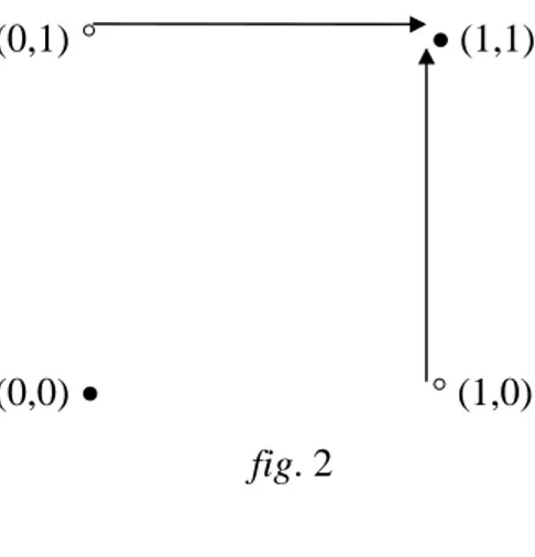
Fig. 2 illustrates the deterministic dynamics of a single sector taken in isolation, on the N = 2, K = 1 fitness landscape described in fig. 1. Black spots identify local peaks of the fitness landscape, hence rest points of the dynamics. The string (1,1) is the global maximum of Vi ( ) on Ai. The string (0,0) has a degenerate basin of attraction, coinciding with the string itself.
(0,1)° • (1,1)
(0,0)• ° (1,0)
fig. 2
Fig. 2 clarifies how the landscape in this example is totally rugged, in the sense that every neighbour of a string that is not a local peak, is an isolated local peak15.
13 Cf. Rosenberg [1976].
14 This amounts to a random selection of one component of x
i, and a change of its configuration (from 0 to 1, or vice
It may be instructive to compare the asymptotic average properties of the ‘blind-exploration’ and deterministic N-K dynamics on randomly generated fitness landscapes for the polar cases of zero and full complementarity. The main differences are as follows (see appendix).
Remark 2.4:
(i) When K = 0, the blind and the deterministic dynamics eventually reach the global peak of the landscape; the number of steps involved is smaller for the latter, because every step is taken in the right direction. The average fitness value V*(N, 0) of the global peak is 0.666 (see proposition 3).
(ii) At 0 < K ≤ N − 1 the blind-exploration dynamics eventually converges to the average local peak of the landscape. The average fitness value V*(N, K) of a local peak changes with N and K as described by proposition 3.
(iii) For N finite, the asymptotic deterministic dynamics on 0 < K ≤ N − 1 landscapes climbs a local fitness peak which is definitely above average. If K = N − 1, the fitness of this above-average peak falls to 0.5, as N tends to infinity16. The same is not true if N grows to infinity, but K is held constant (as implied by proposition 3).
The opening statements of (ii) and (iii) can be most simply illustrated with reference to fig. 1 and 2. There, starting from a random initial state, the global peak is climbed with probability ¾ by the deterministic dynamics and with probability ½ by the blind-exploration dynamics.
Thus, combining proposition 3 and remark 2.4, and assuming that the number N of string components is large, we may conclude that the blind or more intentional character of technological moves does not crucially affect our results. In any case, technical evolution on isolated landscapes assigns a fitness advantage to technical orders with a positive but relatively-low level of input complementarity K. In particular, the K level of the selectively favoured strings is not expected to increase proportionately with N.
16
Indeed, this holds true for the fitness value of every string in the landscape (itself an average of N independent random numbers, because K = N − 1).
3. Technological interdependence across sectors
3.1.
In what follows we consider coupled technological dynamics occurring in S sectors of the economy. We hold temporarily to the simplifying assumption that a single evolving technique (P = 1) is present in each sector. Thus, the state of technique j refers here to the method in use in sector j (j = 1, ..., S). The case where P > 1 is discussed in section 3.2. On any given landscape, the dynamics is assumed to be deterministic, but, in line with the findings of part 2, the same qualitative results hold when the blind-exploration dynamics is considered.
Technological opportunities, input-output interdependence, and spill-over effects imply that, in general, the fitness rank-order list of the 2N states of technique j, depends on the present state of the other S − 1 sectors of the economy. Following Kauffman [1993], we can envisage these effects as deformations of the fitness landscape of sector i, triggered by technical changes in the other S − 1 sectors. More precisely, we shall consider deformations of the fitness-rank-order list of the methods for sector i (i = 1, ..., S). Deformations can be global or local. If interdependence relations across sectors are restricted to small segments of technological strings, a single ‘one-step’ change in one technique in use does not induce a global deformation in the fitness landscape of another technique. However, when the economy consists of many sectors, a multiplicity of ‘one-step’ changes is simultaneously taken. Hence the higher S relative to N, the higher the probability of global deformations. If S is very small relative to N, the case of global deformations rests on the assumption that technological interdependence across sectors is pervasive, as it may be the case when a new general-purpose technology comes into existence. Situations of ‘complete interdependence’ are defined by the fact every component of every technological string is connected to every component of every other string. A single one-step change in one technique is then sufficient to select a completely new landscape (and fitness rank-order list) for every other technique. We shall resort in what follows to this rather extreme assumption, because it suggests a statistical approach to co-evolution, whence the general qualitative effects of complementarity are most easily singled out. For illustration purposes, we shall occasionally refer also to the term ‘strong-interdependence’. This identifies global deformations changing the leading positions in the fitness rank-order list of every technical order.
The coupled technological dynamics of S techniques in the economy is determined by their interdependence pattern; this is the list describing the fitness-rank-order list of each technique corresponding to every technical state of the rest of the economy. The first element in the list is the
fittest. The possibility that contiguous elements in the list have the same fitness is assumed away, because this occurrence would represent an irrelevant fluke. Two examples are shown below for the case where N = 2, S = 2. The two sectors are here called a and b, and, by way of example, a00 is the
technical state (0,0) of sector a. Table 1 refers to the case K = 0, Table 2 to the case K = 1.
if a00: b11, b10, b01, b00 if b00: a10, a11, a01, a00 if a01: b10, b00, b01, b11 if b01: a11, a10, a01, a00 if a10: b00, b10, b11, b01 if b10: a01, a00, a11, a10 if a11: b01, b11, b00, b10 if b11: a00, a10, a01, a11 Table 1 if a00: b00, b11, b01, b10 if b00: a00, a11, a01, a10 if a01: b00, b11, b10, b01 if b01: a00, a11, a01, a10 if a10: b11, b00, b10, b10 if b10: a11, a00, a10, a01 if a11: b11, b00, b10, b01 if b11: a11, a00, a10, a01 Table 2
It is worth observing how Table 1 shows a ‘strong-interdependence’ pattern. We may also notice how, corresponding to the assumption K = 0, there is one and only one local peak in every fitness landscape. Table 2 does not describe a situation of strong interdependence; moreover, each landscape is totally rugged, as allowed by the assumption K = N − 1.
Time is discrete, and at each date every technique moves from the present state to the fittest neighbour (simultaneous moves). The state space of the coupled technological dynamics induced by a given interdependence pattern between S sectors consists of the hyper-cube {0,1}NS. Every hyper-row, or column, of this state space consists of an ordered string of 2N elements, where every element, or point, (x1, ..., xS) is an ordered list of S technical states (strings of N binary codes), one for each sector. A neighbour of a point in state space is an ordered list (y1, ..., yS) such that each yi is a string of N binary codes, and d(xi, yi) ≤ 1. It is easy to see that a point in state space has NS neighbours. Every element of an hyper-row (or column) is therefore a technical state of the economy, and moving on the same hyper-row (or column) we encounter all possible technical states for one sector, while the state of the other S − 1 sectors is unchanged. Recalling that at K = 0 every
fitness landscape has one and only one peak (because we assume away irrelevant flukes) and since, by construction, every hyper-row (or column) refers to the fitness landscape of a given technique, we obtain the following:
Remark 3.1: Assume a given interdependence pattern. A rest point in state space of the deterministic dynamics corresponding to this pattern is such that the S sectors are simultaneously at a fitness peak. If and only if K = 0, on every hyper-row (or column) in the state space there is at most one stationary state.
The ‘only if’ part of remark 3.1 is illustrated in fig. 3 showing the coupled dynamics in state space {0,1}4 determined by the interdependence pattern outlined in table 2.
(a01, b01) (a01, b00) (a01, b10) (a01, b11)
(a00, b01) (a00, b00)• (a00, b10) (a00, b11)•
(a10, b01) (a10, b00) (a10, b10) (a10, b11)
(a11, b01) (a11, b00)• (a11, b10) (a11, b11)•
fig. 3
When K > 0, at a stationary state, the S sectors are not necessarily at the global peak of their landscape (see, for instance, the state (a11, b00) of fig. 3). Some may be at the global peak, while
(a01, b01) (a01, b00) (a01, b10)• (a01, b11)
(a00, b01) (a00, b00) (a00, b10) (a00, b11)•
(a10, b01) (a10, b00)• (a10, b10) (a10, b11)
(a11, b01)• (a11, b00) (a11, b10) (a11, b11)
fig. 4
The number of admissible interdependence patterns depends on the parameters N and K. Since there are 2N different states (strings) of a given technique, there are 2N! different re-orderings of these strings according to their fitness rank-order. When K = N − 1, each of these re-ordrings is admissible. If, instead, K = 0, two contiguous strings on every admissible re-ordering differ in one and only one component. Since every admissible rank-order list for sector h (h = 1, ..., S) can be coupled with 2N(S−1) different states of the rest of the economy, this yields [(2N!) 2N(S−1)]S possible interdependence patterns for the case K = N − 1, and a considerably lower number of possibilities for K = 0. Any admissible pattern gives rise to a deterministic dynamics in phase space, that is a set of 2NS trajectories, each starting from a different initial condition in phase space ( see fig 3 and 4).
Before proceeding with our analysis, it is worth stressing how the properties of evolution on sectoral fitness landscapes taken in isolation, do not generally carry over to the dynamical coupling of evolution on a multiplicity of fitness landscapes. In particular, since each landscape may undergo a deformation at every evolution step, the basins of attraction of the peaks of the isolated landscape do not yield information on the basins of attraction of the stationary states of the co-evolution dynamics. For instance, it may well be the case that at K = 0, all the stationary states in state space have a basin of attraction which is degenerate, in that it coincides with the rest point. This is
illustrated in fig. 4 showing the dynamics in state space following from the (strong) interdependence pattern of table 117.
A randomly selected interdependence pattern results from 2N(S−1) independent draws (with re-introduction) of a fitness rank-order list for sector i (i = 1, ..., S), one for each technical state of the rest of the economy. As before, we may think of these lists as uniformly distributed on their support. Once a given pattern is fixed, the dynamics in phase space is fully deterministic. However, we can investigate how the parameters N and K affect the relative frequency with which the dynamics in phase space converges to a stationary state, over the set of all possible interdependence patterns. By construction, every pattern is as likely as any other.
Remark 3.2: Assume complete interdependence as defined in section 3.1. The probability that the S sectors are simultaneously at a fitness peak after a random draw of their landscape is 1/2NS, if K = 0, and 1/(N + 1)S, if K = N − 1. Thus, the expected number of stationary states in phase space is 2NS/2NS = 1 and 2NS /(N + 1)S, respectively. (This follows trivially from remarks 2.1, 2.2.)
Remark 3.3: A dynamics in phase pace corresponding to a given interdependence pattern can be regarded as a directed graph Γ with the following properties: (i) Points in phase space are vertices of the directed graph, these vertices being ordered to form hyper-rows and columns. (ii) Every vertex of Γ has at most one exiting edge, and every directed edge connects one vertex to a neighbouring vertex. (iii) Stationary states correspond to vertices with non-exiting edges. (iv) There are not neighbouring vertices with non-exiting edges on the same hyper-row or column. (v) Consider four mutually neighbouring vertices disposed on their adjacent hyper-rows and columns to form the vertices of a rectangle. Any two such vertices are opposite, if they do not share a side of the rectangle. Then: (a) if two opposite vertices are connected by a diagonal directed edge, the same can not hold for the other couple of vertices; (b) two exiting edges disposed on parallel sides of the rectangle do not point to the same hyper-row or column; (c) a vertex sharing a side of the rectangle with a vertex x without exiting edges, can not have its exiting edge pointing to the vertex of the rectangle which is opposite with respect to x.
For fixed N and S, the set of dynamics that are admissible under K = 0 correspond to the set of graphs meeting the properties outlined in remark 3.3 and such that every hyper-row and column has at most one vertex with non exiting edges. If K = N − 1, the maximum number of vertices with non-exiting edges on the same hyper-row or column is only constrained by condition (iv) above.
It is then easy to verify that on the set of dynamics that are admissible for K = N − 1, the relative frequency of the trajectories meeting a stationary state is higher than on the set of dynamics that are admissible for K = 0. More generally, the probability of convergence to a stationary state is
17
Symmetrically, it is quite easy to produce examples where, at S = 2, N = 2, K = 1, the ruggedness of fitness landscapes is sufficient to rule out the occurrence of degenerate basins of attraction, even in situations of strong
an increasing function of the frequency of such equilibria in state space, hence it increases with the ratio K/N, as stated by proposition 3.
Remark 3.3: Assume complete interdependence as defined in section 3.1. Then, the expected asymptotic fitness of a technique, conditioned on the convergence of the asymptotic dynamics to a stationary equilibrium in state space, is the expected fitness value of a local peak of the given technique.
Remark 3.4: Since the state space is finite, the deterministic dynamics corresponding to any given interdependence pattern either converges to a stationary state, or to a periodic orbit. Assume complete interdependence as defined above. For N finite, the results of part 2 imply that the expected fitness of a given technique is lower on the set of periodic orbits (of all possible interdependence patterns), than it is at local peaks. The above fitness differential tends to zero as N increases with K = N − 1.
We are now ready to state the main result of this section.
Proposition 4. Assume complete interdependence as defined above and consider the expected asymptotic fitness of S co-evolving techniques as a function of N and K. If N ≥ 2 the expected asymptotic fitness of a co-evolving technique is maximized at K > 0. If N is sufficiently large, then the expected asymptotic fitness of a co-evolving technique is maximized at K positive and lower than N − 1.
3.3.
In this section we drop the assumption P = 1, and allow for a multiplicity of technical orders which compete in each sector to settle as dominant designs. On the premise of the forgoing analysis, and of the body of evidence presented in Kauffman [1993], we expect that in a process of technological co-evolution where many techniques are competing in each sector, the probability that a technique eventually settles as a dominant design is not independent of its degree of complementarity K. In particular, techniques with a very low degree of complementarity should be selected against in a process of co-evolution where N ≥ 2. A prototype experiment has been designed to test this prediction of the theory. To the best of our knowledge, the experiment is new in that the K value of the techniques with which any technique may interact is not pre-defined. This is because inter-sectoral effects originate from the methods ‘in use’ and in the course of evolution the changing methods and techniques ‘in use’ are characterized by different K values.
A method is a configuration within a given technique. A technical state of S sectors is a list of S methods in use, one for each sector. The wording ‘method in use’ refers to the fact the method, and the corresponding technique, is adopted by a majority of firms in the given sector. In this
respect, we distinguish between exploration and imitation. As it was the case in the previous sections, the exploration of a given method cannot perceive technical opportunities beyond those contained in the neighbourhood of the present technical configuration. Possibility of imitation of the currently observable technical states is introduced to interpret the assumption that the technique yielding the technical configuration which is currently ‘best practice’ in sector i, is also the technique currently ‘in use’ in sector i (i = 1, ..., S). Techniques that are not jet ‘in use’ may also evolve; hence, we are concerned with the state of the SP techniques in the economy.
We considered P = 3 competing techniques in each sector. Their K values were K = 0, K = N/2, K = N − 1, respectively. Given our constraints on computing resources we fixed S = 2, N = 10. Technical interdependence across sectors was introduced by assuming that the fitness contribution of each component of each of the P techniques in one sector, is conditioned by the configuration of C = 3 components of the method in use in the other sector. Each co-evolution experiment was run for 40 steps. In each sector, on a sample of 100 experiments, the average fitness value at the last step is maximal for the technique with K = N/2. Details of the Mathematica program with which the simulation experiment has been run are given in appendix A.3.
4. Conclusion
A number of stilized facts emphasized by historians of technological change are worth recalling in connection to the analysis above.
Most important is that the transition between alternative technology systems (think of the transition from water and steam power generation to electricity, or the advent of the computer substituting for traditional forms of information transmission) is marked by a period of high technological uncertainty (Rosenberg [1996]) which lasts until the emergence of sufficiently stable, hence widely understood, dominant designs (Anderson and Thusman [1990]). This type of uncertainty is strictly related to the re-orientation and the co-evolution of technological opportunities after a pervasive technological breakthrough, with the effect that the full potential of the new technology system and, relatedly, the ‘right’ channels of investment, are impossible to foresee in advance.
It should be noted in this respect that the foregoing analysis, based, as it is, on the expected asymptotic fitness corresponding to different K/N ratios, may grossly under-estimate the benefits from a higher probability of attaining a stationary state. A relevant part of these benefits has to do with the lower average number of failed innovation efforts during the transitional dynamics.
Current economic analyses of the trajectory determined by the advent of a macro-invention or a new general-purpose technology (see, for instance, Helpman and Trajtenberg [1994], Helpman [1998]) emphasize how time-and-resource-consuming innovation effort in the development of complementary inputs is required before the new technology takes off and reaches its full potential. In comparison to these analyses, the above model lays more emphasis on technological uncertainty due to co-evolving opportunities, and the related possibility of mis-directed investment. This adds a further dimension to current explanations of well known phenomena, such as the relatively long delay of the productivity-take-off after a technological revolution. In the first place, the competition between the alternative designs may take a substantial amount of time before a winner emerges18. In the second place, at the time when a dominant design emerges, substantial outlays of fixed-capital stock embodying the different designs, that failed to become dominant, are already in place. Even when they can be kept in place, till they wear out, their adaptation to the dominant design is not free of cost19. The perspective adopted in this paper brings then to the fore a further and probably under-estimated source of slower productivity growth during a technological transition.
From a higher stand point, a further, but still open issue raised by Kauffman’s work is concerned with the way in which complementarity itself is kept under control within a co-evolution process. For a given scale of N, of the number of co-evolving strings S, and inter-acting components C, if parameter K is sufficiently ‘low’, the model ecosystem tends to exhibit a complex dynamics with irregular oscillations; if K is sufficiently large the model ecosystem reaches a frozen state where the S strings are simultaneously at a fitness peak. But the level of K of an individual in a species, or technique, is itself affected by mutations20. Kauffman’s bold hypothesis is that in view of the trade-off between the probability of converging to a fitness peak and expected altitude of this peak, model ecosystems exhibit a self-organizing property which tends to locate them in a parameter range near the border between the complex and the ordered regime (self-organized criticality). The ability of Kauffman’s N-K-C-S model to exhibit such a property has been questioned (Bak [1996]) on the ground that the emergence of criticality requires the ad-hoc thin choice of the interaction parameter C. Bak [1996] (see also the references quoted therein) presents a
18 For instance, the ‘battle of the systems’ of direct and alternating current generation and transmission lasted about ten
years, before the latter clearly emerged as the likely winner (Hughes [1983]).
19 Drawing again an example from the history of the electric-supply industry, we may recall that the equipment designed
to distribute direct current to final consumers had to be adapted to the poliphase, alternating-current, large-area supply system. This entailed the introduction of step-down trasformers and converters (Hughes [1983]). In post World War I Britain, the adaptation to the new national grid of the Newcastle upon Tyne regional supply system, which had successfully operated before the war, also entailed substantial costs (Hughes [1983]).
20 In terms of our technological interpretation, a breakthrough is followed by the birth (speciation) of multiple technical
route to self-organized criticality in a very simple model of Darwinian selection, where Kauffman’s N-K architecture disappears. (An application in the technological domain is Arenas A., Diaz-Guilera A., Perez J. C., Vega-Redondo F. [1999].) Thus, the relation between input complementarity, as defined in this paper, and self-organized criticality is still an open area of research.
Appendix
A.1.
Proof of Proposition 2: Suppose not. Then, if xi is a maximum of Vi( ) on Ai, there may be in the same space an isolated maximum (either local or global) yi ≠ xi of the fitness function Vi( ). By construction, Vi() has a non-monotonic behaviour on every minimal path joining yi to xi. This contradicts proposition 1, thus completing the proof.
A.2.
Proof of Proposition 3: We are left to prove statements (ii) and (iii).
(ii) Since K = N − 1, fitness values are uncorrelated; each string in the landscape has a probability 1/(N + 1) of being a local peak, and the expected number of local peaks is 2N/(N + 1). In every landscape, the lowest local peak has a fitness value higher than the fitness value of at least N other strings (its N neighbours). The fitness value of the global peak can be thought of as the maximum in a set of 2N fitness values. This yields lower and upper bounds to V*(N, N − 1):
E [Max(a1, a2, ..., am)] < V*(N, N − 1) < E [Max(b1, b2, ..., bM)]
where each aj and bjis an average of N random numbers in the unit interval, m = N + 1, M = 2N . Since the expected fitness values of ‘intermediate’ local peaks are uniformly distributed between the lower and upper bounds above, we have:
V*(N, N − 1) = {E [Max(a1, a2, ..., am)] + E [Max(b1, b2, ..., bM)]}/2
Order statistics shows that {E [Max(a1, a2, ..., am)] + E [Max(b1, b2, ..., bM)]}/2 ≈ 0.7. for 4 ≤ N ≤ 10. Thereafter, V*(N, N − 1) declines as N increases and converges to 0.5 as N grows to infinity, because each single sample average aj, bj must behave accordingly.
(iii) Let K = N − 1 and consider V*(N, K) at N = mN, and K = K. Through a possible re-ordering of components, every string of length N can be thought of as being composed of m segments of N components each. Within each segment each component is connected to the K other components. Thus, the fitness contribution of each component depends on its configuration (0 or 1) and on the configuration of every other component of the same segment. Hence the expected fitness contribution of each segment is an average of N random numbers in the unit interval and is identical to the expected fitness contribution of every other segment. This holds independently of the size of m.
orders are characterized by fluctuations in the level K around an average level (which may depend on the nature of the
The string {x1, ..., xN, xN + 1, ..., x2N, ..., xmN} is at a local peak if and only if each of the m segments is at a local peak. Thus, the expected fitness value of a local peak of {x1,..., xmN} is the expected fitness value of a local peak of any of its m segments. This completes the proof.
A.3
Details of the Mathematica program used for the simulation reported in section 3.4. Here s refers to the number of techniques in each of the two sectors.
s=3;n=10; k={0,n/2,n-1,0,n/2,n-1}; f[m_,y_,x_,tm_,h_]:= Flatten[{m[[x,y]],If[y+k[[x]]<n+1,Take[m[[x]], {y+1,y+k[[x]]}],Flatten[{m[[x]][[Range[y+1,n]]], m[[x]][[Range[1,k[[x]]-n+y]]]}]],tm[[If[x<s+1,2,1]]][[Range[1,h]]]}]; fittab[y_,x_,p_,h_]:= (SeedRandom[x*s*n+y+p]; Table[Random[],{2^(k[[x]]+1+h)}]); xfit[m_,x_,tm_,h_]:=Table[fittab[y,x,p,h][[(Sum[ (f[m,y,x,tm,h][[i]])*2^(k[[x]]+1+h-i),{i,1,Length[f[m,y,x,tm,h]]}] +1)]],{y,1,n}]; totfit[m_,x_,tm_,h_]:=Apply[Plus,xfit[m,x,tm,h]]/n; neigb[m_,x_]:=Prepend[Table[ReplacePart[m[[x]],1-m[[x,i]],i], {i,1,n}],m[[x]]]; fitneigb[m_,x_,tm_,h_]:=Table[totfit[ReplacePart[m,neigb[m,x][[q]], x],x,tm,h],{q,1,n+1}]; fitlist[m_,tm_,h_]:=Table[totfit[m,i,tm,h],{i,1,2*s}]; next[{p_,m_,ch_,tm_,fl_}]:={p, Table[neigb[m,x][[Position[fitneigb[m,x,tm,h], Max[fitneigb[m,x,tm,h]]][[1,1]]]],{x,1,2*s}], {Position[fitlist[m,tm,h] [[Range[1,s]]],Max[fitlist[m,tm,h][[Range[1,s]]]]][[1,1]], s+Position[fitlist[m,tm,h][[Range[s+1,2*s]]], Max[fitlist[m,tm,h][[Range[s+1,2*s]]]]][[1,1]]}, m[[{Position[fitlist[m,tm,h] [[Range[1,s]]],Max[fitlist[m,tm,h][[Range[1,s]]]]][[1,1]], Position[fitlist[m,tm,h][[Range[s+1,2*s]]], Max[fitlist[m,tm,h][[Range[s+1,2*s]]]]][[1,1]]}]], fitlist[m,tm,h]}; m=(SeedRandom[1];Table[Table[Random[Integer],{n}],{2*s}]); tm=m[[{1,s+1}]];ch={1,s+1};h=3;fl=Table[0,{6}]; Sum[Nest[next,{p,m,ch,tm,fl},40][[5]],{p,1,100}]/100
References
Anderson P. and Thusman M. [1990]: “Technological Discontinuities and Dominant Designs: A Cyclical Model of Technological Change”, Administrative Science Quarterly, vol. 35, pp. 604-33.
Antonelli C. [1994]: “Localized Technological Change and the Evolution of Standards as Economic Istitutions”, Information Economics and Policy, vol. 6.
Arenas A., Diaz-Guilera A., Perez J. C., Vega-Redondo F. [1999]: “A self-organized model of technological progress”, Mimeo.
Bak P. [1996]:How Nature Works: The Science of Self-Organized Criticality, Copernicus, New York. Campbell D. T. [1960]: “Blind Variation and Selective Retention in Creative Thought as in other
Knowledge Processes”, reprinted in Radnitzky and Bartley (eds.) [1987], pp. 91-114.
David P. [1990]: “The Dynamo and the Computer: An Historical Perspective on the Modern Productivity Paradox”, American Economic Review, Paper and Proceedings, vol 80, 2, pp. 355-61.
David P. [1992]: “Heroes, Herds and Hysteresis in Technological History: Thomas Edison and the Battle of the Systems Reconsidered”, Industrial and Corporate Change, vol.1, pp. 129-180.
Devine W. [1983]: “From Shafts to Wires: Historical Perspective on Electrification”, The Journal of
Economic History, vol. XLIII, pp. 347-72.
Dosi G. [1997]: “Opportunities, Incentives and the Collective Patterns of Technological Change”, Economic
Journal, vol. 107, pp. 1530-47.
Freeman C. (ed.) [1990]: The Economics of Innovation, Aldershot and Brookfield, Elgar Reference. Ghiselin B. (ed.) [1952]: The Creative Process, Berkeley, University of California Press.
Gould S. J.[1992]: “The Panda’s Thumb of Technology”, in S. J. Gould, Bully for Brontosaurus, Harmondsworth, Penguin Books.
Helpman E. [1998]: General Purpose Technologies and Economic Growth, Cambridge, Mass., MIT Press. Helpman E. and Trajtenberg M.[1994]: “A Time to Sow and a Time to Reap: Growth Based on General
Purpose Technologies”, NBER Working Paper #4854.
Hughes T. P. [1983]: Networks of Power. Electrification in Western Society, Baltimore, John Hopkins Univ. Press.
Kauffman S. [1993]: The Origins of Order, New York, Oxford Univ. Press.
Landau R., Taylor L., Wright G. (eds.), [1996]: The Mosaic of Economic Growth, Stanford, Stanford University Press.
Levinthal D. [1997]: “Adaptation on Rugged Landscapes”, Management Science, vol. 43, pp.934-50.
Marschak T. and Nelson R. [1962]: “Flexibility, Uncertainty and Economic Theory”, Metroeconomica, 14, pp. 42-58.
Metcalfe J. S., Miles I. [1994]: “Standards, Selection and Variety: an Evolutionary Approach”, Information
Economics and Policy, vol. 6, pp. 243-68.
Milgrom P. and Roberts J. [1990]: “The Economics of Modern Manufacturing: Technology, Strategy and Organization”, The American Economic Review, vol.80, pp.511-28.
Mokyr J. [1990]: The Lever of Riches, New York, Oxford Univ. Press.
Mokyr J. [1991]: “Evolutionary Biology, Technological Change and Economic History”, Bulletin of Economic Research, vol.43, pp. 127-49.
Nelson R. and Wolff E. [1997]: “Factors Behind the Cross-Industry Differences in Technical Progress”,
Structural Change and Economic Dynamics, vol. 8, pp. 205-220.
Pagano U. [1998]: “The Origin of Organizational Species”, Quaderni del Dipartimento di Economia
Politica, University of Siena.
Poincaré H [1908]: “Mathematical Creation”, reprinted in Ghiselin (ed.) [1952], pp 23-33.
Radnitzky G. and Bartley W. W. III (eds.) [1987]: Evolutionary Epistemology, Rationality, and the
Sociology of Knowledge, La Salle, Ill., Open Court.
Rosenberg N. [1976]: Perspectives on Technology, Cambridge, Cambridge University Press.
Rosenberg N. [1996]: “Uncertainty and Technological Change”, in Landau, Taylor, Wright (eds.) [1996]. Utterback J. and Abernathy W. [1975]: “A Dynamic Model of Process and Product Innovation”, Omega,
vol. 33, pp. 639-56, re-printed in Freeman (ed.) [1990], pp. 424-41.
Westhoff H., Yarbrough B. and Yarbrough R. [1996]: “Complexity, Organization, and Stuart Kauffman’s
The Origins of Order”, Journal of Economic Behaviour and Organization, vol. 29, pp. 1-25.