Optimization Techniques for Stencil Data Parallel Programs: Methodologies and Applications

(1)

University of Pisa and Scuola Superiore

Sant’Anna

Master Degree in Computer Science and Networking

Corso di Laurea Magistrale in Informatica e Networking

Master Thesis

Optimization Techniques for

Stencil Data Parallel Programs:

Methodologies and Applications

Candidate

Supervisor

Andrea Lottarini

Prof. Marco Vanneschi

(2)

(3)

List of Figures

1.1 Graphical representations of the functional dependencies of respectively Jacobi and Jacobi with applied Q trasformation stencils . . . 4 2.1 The process of finding an approximate solution to the PDE

via the Finite Difference Method. . . 11 2.2 Three-point stencil of centered difference approximation to the

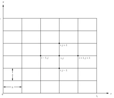
second order derivative. This stencil represents Equation 2.3. 12 2.3 Discretization of temperature over a flat surface. The domain

is divided into rectangles of width h and height k. . . 16 2.4 Five-point stencil for the centered difference approximation to

Laplacean. . . 16 2.5 Graphical depiction of periodic boundary conditions( Figure

2.5a ) and constant boundary conditions ( Figure 2.5b ) of a 3x3 mesh. . . 21

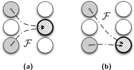
3.1 Framework for stencil computations as presented in [31]. . . . 30 3.2 Graphical depiction of the functional dependencies of Laplace

stencil computation ( Figure 3.2a ) and its partition depen-dencies ( Figure 3.2b ). . . 31 3.3 Perimeter of a partition with respect to partition area for row

and block partitioning in a 2 dimensional working domain. . . 34 3.4 Dependencies between partitions with respect to parallelism

degree for row or block partitioning in a two dimensional work-ing domain. . . 34 3.5 Pseudocode representation of the Laplace stencil at the

con-current level. Partitions (or processes) are labelled by means of the coordinates with respect to the actual partition. . . 36 3.6 Pseudocode representation of the Laplace stencil at the

con-current level. With respect to concon-current code shown in Figure 3.5, we have that communication and computation overlaps. . 37

(6)

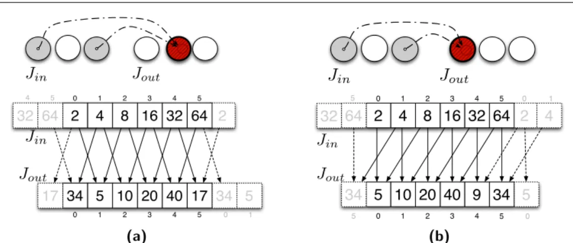
4.1 Graphical depiction of a time step of a mono dimensional ja-cobi stencil on a toroidal grid (Figure 4.1a) and a positive Q trasformation of the same stencil ( Figure 4.1b). . . 40 4.2 Graphical depiction of the incoming functional dependencies

of Laplace stencil computation with positive Q Transforma-tion applied. . . 41 4.3 Graphical depiction of Partition dependencies in the case of

the Laplace stencil (Figure 4.3a) and Laplace stencil with ap-plied Q trasformation (Figure 4.3b). Incoming (Figure 4.3d) and outgoing (Figura 4.3c) communications at the concurrent level with respective regions. . . 43 4.4 Graphical depiction of two time steps of a mono dimensional

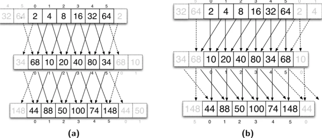
jacobi stencil on a toroidal grid (Figure 4.4a) and the same computations with a positive Q trasformation applied in the first time step and a negative Q trasformation applied at the second step ( Figure 4.4b). The stencil kernel is the sum of the two elements of the shape. Notice that the final displacement of output values is correct. . . 44 4.5 Graphical depiction of functional dependencies in the case of

naive jacobi stencil (Figure 4.5a) and the Jacobi stencil with applied positive QM trasformation(Figure 4.5b). . . 46 4.6 _{QM transformation of the one dimensional jacobi stencil}

com-putation presented in Figure 4.5. . . 46 4.7 Graphical depiction of the incoming communications of Laplace

stencil computation (Figure 4.7a). Graphical depiction of the outgoing communications ( Figure 4.7b ) with QM trasfor-mation applied. . . 47 4.8 Execution of transformed Laplace Stencil with_QM

trasforma-tion(Figure 4.8a). Execution of transformed Laplace Stencil with QW trasformation(Figure 4.8b) . . . 49 4.9 Graphical representation of incoming communications (fig. 4.9a)

and outgoing communications (fig. 4.9b) of the nine point stencil. . . 52 4.10 Graphical representation of the incoming communication

pat-tern (fig. 4.10a) and outgoing communication patpat-tern (fig. 4.10b) of the nine point stencil with shift method applied. Numbering reflects the order of the communications needed to preserve correctness. . . 52 4.11 Communication patterns of a generic stencil computation (left)

compared with the same computation with oversending method applied (center) and with a _{Q trasformation applied (right). . 56}

(7)

List of Figures

4.12 Step Fusion method applied to the two dimensional Jacobi stencil computation. . . 57

5.1 Extended reference model. . . 63 5.2 Memory accesses with increasing step fusion factor in Jacobi

computation. . . 65 5.3 Number of cache miss (normalized with respect of the number

of time steps) for different size of the data matrix and a fixed number of cache locations (1k). . . 66 5.4 Elements accessed by the naive and the SF version of the

ja-cobi 2d stencil. Red elements are updated by the naive version. Blue elements are updated by the _{SF version. . . 67} 5.5 Pattern of accesses to matrix A of Listing 5.9 . . . 72 5.6 Convex polyhedron which represent the iteration space of

List-ing 5.10 . . . 73 5.7 Reuse of a generic element of the mesh in a jacobi 2d stencil. . 76 5.8 Graphical depiction of the optimized schedule of the two

di-mensional jacobi stencil . . . 77 5.9 Figure 5.9b shows a graphical depiction of the pattern of

up-dates in a optimized schedule for the 3d Laplace stencil shown in Figure 5.9a. . . 78 5.10 Graphical depiction of time skewing applied to a

monodimen-sional laplace stencil. . . 79 5.11 Area of a trapezoid (cache block) for a generic mono

dimen-sional stencil . . . 80 5.12 Projection of a 3d space time lattice for a skewed 2 dimensional

stencil with order equal to one. . . 82 5.13 Time skewing that has to be reduced because the number of

time steps is not sufficient. The optimal trapezoid (dotted) would have been substantially bigger than the actual trape-zoids (shaded) . . . 83 5.14 A generic trapezoid. As usual, the two slopes are derived from

the data dependencies of the computation. . . 84 5.15 Figure 5.15a shows a graphical depiction of a space cut. Figure

5.15b shows a graphical depiction of a time cut. . . 84

6.1 Number of cache miss with respect to step fusion level. The optimal value corresponds to M2_{/B. Matrix has a size of} 2048x2048 and the cache has a size of 1024 elements. . . 91

(8)

6.2 Graphical depiction of time skewing on a mono-dimensional stencil. Different trapezoids should be executed from left to right. . . 94 6.3 Graphical depiction of parallel time skewing. Different

trape-zoids belongs to different workers. The space-time portions labelled as “clean up work” should be updated after the adja-cent trapezoids. . . 95 6.4 Circular Queue optimization of a time skewed mono

dimen-sional stencil. . . 95 6.5 Execution of three steps of the proposed modified version of

time skewing. . . 96 A.1 Mean completion time of a single time step of the naive, Q

, _{Q and SH versions of the two dimensional Jacobi stencil} executed on Andromeda. . . 100 A.2 Communication time of a single time step of the of naive, Q

, _{Q and SH versions of the two dimensional Jacobi stencil} executed on Andromeda. . . 101 A.3 Computation time of a single time step the of naive,Q , Q and

SH versions of the two dimensional Jacobi stencil (without MPI communications) executed on Andromeda. . . 102 A.4 Mean completion time of naive of the naive Q and Q + SH

version of the Jacobi stencil executed on Titanic. . . 102 A.5 Total, computation and communication time of the two

di-mensional jacobi stencil (naive version) executed on Titanic. . 103 A.6 Mean completion time of naive and_{Q + SH version of the 3d}

Jacobi stencil executed on Andromeda. . . 104 A.7 Mean completion time of naive,SF2 _and _SF2 ₊_{SH version}

of the Jacobi stencil executed on Titanic. Values are normal-ized w.r.t the number of time steps. . . 105 A.8 Comparison of Computation cost for both naive andSF2

ver-sion. Communication cost of the naive version is shown for reference. Notice that for sufficiently big partitions the com-putation cost dominates. . . 105 A.9 Comparison of naive, loop tiling and time skewing version of

the two dimensional laplace stencil. . . 106 A.10 Speedup (Tnaive/Topt) of loop tiled and time skewed version

with respect to the naive version of the two dimensional laplace stencil. . . 107

(9)

Listings

1.1 Pseudocode of a Jacobi update for the resolution of a two dimensional poisson equation. . . 2 1.2 Pseudocode of reordered Jacobi update for the resolution of a

two dimensional poisson equation. . . 3 2.1 Pseudocode of a generic map computation. The computation

is defined over 4 time steps. . . 7 2.2 Pseudocode of the implementation of the map computation

presented in Listing 2.1. Two real data structures are used and elements are updated sequentially. . . 8 2.3 Pseudocode of Laplacian Operator. . . 9 2.4 Pseudocode of a Jacobi Iteration for matrix equation 2.7. . . . 13 2.5 Pseudocode of a Gauss Seidel Iteration for matrix equation 2.7. 14 2.6 Pseudocode of a Red Black Gauss Seidel Iteration for matrix

equation 2.7. . . 15 2.7 Pseudocode of Jacobi method for the linear system 2.18. . . . 18 4.1 Pseudocode representation of a two dimensional nine point

stencil, which has dependencies with every surrounding parti-tion. Partitions (or processes) are labeled by means of coordi-nates with respect to the examined partition. . . 51 4.2 Pseudocode representation of a two dimensional laplace stencil

with oversending method applied. . . 55 5.1 Pseudocode of naive 2d Jacobi stencil. . . 62 5.2 Pseudocode of 2d Jacobi stencil with applied_{SF method. . . 62} 5.3 Code of a mono dimensional laplace operator . . . 70 5.4 Loop unrolling of Listing 5.3 . . . 70 5.5 Pseudocode that computes the sum of the columns in a matrix.

We are assuming that the matrix A is stored in memory in row order. . . 70 5.6 Pseudocode of the Loop Interchanged version of the algorithm

shown in Listing 5.5 . . . 70 5.7 Pseudocode of the matrix vector multiplication . . . 71

(10)

5.8 Pseudocode of the matrix vector multiplication with innermost loop tiled. b is a multiple of block size B. . . 71 5.9 Pseudocode of the matrix vector multiplication with both loops

“tiled”. . . 72 5.10 Generic for loop with loop conditional as affine functions. . . . 73 6.1 Pseudocode representation of a generic structured grid

com-putation defined at the concurrent level. The working domain is defined in two dimension and has size M xM . Depending on the stencil shape some of the SEND and RECV operations might not be necessary. . . 88 6.2 Nested loops for the update of the incoming independent

re-gion of a two dimensional Jacobi stencil. . . 89 6.3 Nested loops for the update of the incoming independent

re-gion of a two dimensional Jacobi stencil with SF applied. . . 89 6.4 Pseudocode representation of a generic two dimensional stencil

(η = 1) with shift method applied. Not all SEND and RECV operation might be necessary depending on the stencil’s shape. 92 6.5 Pseudocode representation of a generic two dimensional stencil

(η = 1) with oversending method applied. Not all SEND and RECV operation might be necessary depending on the stencil’s shape. . . 93

(11)

Chapter 1 Introduction

Data Parallelism is a well known form of parallelization, which is based on partitioning the data across different parallel computing nodes. Its relevance will increase in the near future because of two joint factors. The first factor is the industry switch to parallel microprocessors. The second factor is the subtle and constant transition from control intensive computations to data intensive computations driven by the massive amount of information gener-ated today[4]. One of the most challenging open problems is the optimization of such computations in order to ensure the desired performance and hope-fully, portability of performance, among the diverse set of future computer architectures. In order to investigate the difficulties of optimization, we se-lected a subset of all data parallel computations known as structured grid computations[4]. As we will see in the next section, structured grids are cen-tral for many simulation codes; therefore, they were studied extensively in the high performance computing community. Although they are relatively simple computations in terms of structure, their optimization is a difficult process and many different solutions were proposed in literature. Because of these complications, no standard libraries or frameworks exist for structured grid computations while almost standard solutions exist for dense linear alge-bra (ATLAS[43]), sparse linear algealge-bra (OSKI[42]) and spectral (FFTW[19]) computations.

1.1 Structured Grid Computations

Partial differential equation (PDE) solvers constitute a large portion of all scientific applications. PDE solvers are at the heart of simulation codes for many areas, from physical phenomena[27] to financial market stock pricing[22]. In order to solve partial differential equations, one possible approach is the

(12)

finite difference method[28]. In this method, the differential operators are approximated by truncated Taylor expansions of their derivatives and the continuous domain where PDEs are defined is discretized. This results in a very sparse matrix equation with predictable entries that can be solved efficiently by using iterative methods. Iterative methods find the solution by repeatedly updating an initial guess until numerical convergence is achieved. Each point is updated with a weighted contributions of its neighbours. Con-sider as an example a two dimensional poisson equation: ∆u = f where f is a known function. After applying the finite difference method its solution can be found by updating an initial guess with the Jacobi iterative method until the error is below a given threshold. The pseudocode of a single jacobi update is shown in Listing 1.1.

for i = 1 .. n for j = 1 .. n

unew[i][j] = (f [ i ][ j ] − uold[i−1][j] − uold[i+1][j] − uold[i][j+1] −

uold[i][j+1])/4

Listing 1.1: Pseudocode of a Jacobi update for the resolution of a two dimensional poisson equation.

These solvers can be easily implemented in a data parallel fashion where different workers update different portions of the result for the next time step.

Given the regularity of these computations, they are called structured grid computations. Computations in this class range from very simple Jacobi iterations (Listing 1.1) to multigrid[9] or adaptive mesh refinement methods[7]. We chose structured grids computations as a benchmark for optimization methods for data parallel computations because of two factors:

1. They are fundamental for a wide set of simulation codes in multiple disciplines.

2. Although they are very simple, these computations usually achieve a fraction of their theoretical peak performance on modern architectures[25].

Therefore, the optimization of these computations has been the subject of much investigation. In particular, previous research has shown that mem-ory transfers constitute the main bottleneck for this class of computations. Therefore, research focused primarily on tiling optimizations that attempt to reduce the memory traffic by increasing the temporal locality (reuse) of the computation. Tiling optimizations constitute a subset of the class of loop reordering transformations. Loop reordering transformations modify the

(13)

Chapter 1. Introduction

order in which updates are executed. Assuming a row order storage of data, we could reorder the computation in Listing 1.1 in the following way:

for jj = 1,B,n for i = 1 .. n

for j = jj .. jj + B − 1

uold[i][j+1])/4

Listing 1.2: Pseudocode of reordered Jacobi update for the resolution of a two dimensional poisson equation.

Since the updates of the Jacobi method can be performed in any order, the transformed program will produce the same result. Moreover, by selecting a good parameter B we can reduce the number of cache miss. A formalization of this method, together with a rigorous analysis, is presented in Chapter 5. Initial research focused on tiling only the spatial dimension[34] (Listing 1.2). However, reuse in structured grids computations is relatively limited compared to classic methods for dense linear algebra. In fact, further research has shown that tiling also in the time dimension (time skewing) gives the best results[24]. A comprehensive analysis of different tiling techniques was presented in [14].

The effectiveness of tiling is strictly related to an optimal selection of the tile sizes. Sophisticated models were introduced in order to solve this problem[25]. However, peculiarities of modern architectures makes formal modelling of this problem difficult. In fact, research has focused on auto-tuning techniques in order to select an optimal set of parameters without having to derive a formal model[15, 13]. Another possible approach is to use cache oblivious algorithms. A cache oblivious time skewed algorithm for d-dimensional structured grids was presented in [20, 21]. The idea behind cache oblivious algorithms is to recursively divide the working domain so that almost optimal tile sizes are selected for a given level of recursion thus, making the algorithm oblivious to the problem size or the specifications of the cache hierarchy. Recently, a compiler for stencil computations using a cache oblivious approach was presented[38].

Some optimizations methods, specific to structured grid computations were recently developed in our HPC lab[29, 31]. Unlike other methods present in literature, these methods attempt to reduce the overhead of communica-tions between processors by slightly modifying the computation. As a exam-ple consider the code in Listing 1.1 which can be graphically represented as in Figure 1.1a. The_{Q trasformation presented in [31] modifies the functional} dependencies of the computation and produces the shape in Figure 1.1b.

(14)

(1, 0) (−1, 0) (0, 1) (0, −1) (a) (1, 0) (0, 1) (2, 1) (1, 2) (b)

Figure 1.1: Graphical representations of the functional dependencies of respec-tively Jacobi and Jacobi with applied Q trasformation stencils

These optimizations are presented in Chapter 4. Unfortunately, research on specific methods for parallel stencil codes on distributed memory ma-chines is very limited[35]. Some methods were presented in order to reduce the number of communications among parallel executors[17, 33]. Overall, the work of Meneghin[31] is the most comprehensive in this specific context. In particular, it presents transformations for structured grids that ensure a minimal number of communications and occupation of memory among all techniques found in literature. We present them, together with standard methods found in literature, in a structured model extended from [31]. A cost model is used to derive theoretically the performance gain of different optimizations. In particular, for tiling optimizations, we show that it is pos-sible to reduce the number of memory accesses to the order of the theoretical lower bound. Moreover, their interaction with transformations presented in [31] is analyzed in detail and solutions are presented in order to maintain the benefits of both classes of optimizations.

Methodology We claim that a structured model is necessary to study the interaction of different optimizations. Optimizations are often presented in a non-structured way where benefits are elucidated in an intuitive way and then experimental results are used to prove the optimization’s suitability. Instead, we selected a simple cost model derived from [40]. The cost for a program is the maximum between the cost of communication and com-putation TC = max(Tcalc, Tcomm). We are assuming that we can overlap completely computation and communication. Tcalc is the maximum of the number of memory access among different processes in an external memory model. Tcomm is derived by associating a fixed cost to every communication Tsetupand a variable cost that depends on the message size, Ttrasm. So a

(15)

com-Chapter 1. Introduction

munication of m elements between two workers will have an associated cost of Tsetup+ m∗ Ttrasm. By using such model, it is possible to show the perfor-mance gain of optimizations without meddling with peculiarities of modern architectures. Moreover, we are able to study the interaction of the different methods, which were analyzed individually.

1.2 Thesis Outline

Data parallel computations are presented in Chapter 2. Structured grids are examined in detail in the same chapter. Their relevance is demonstrated with real world examples and typical properties of a structured grid compu-tations are described. The structural model that we used to present different optimizations is introduced in Chapter 3. This model is general in order to represent any framework for a class of computations. Moreover, a spe-cific instance of the model for structured grids computations, along with a concretion and optimization examples, are illustrated. Optimizations for a parallel implementation of structured grids are introduced in Chapter 4. Most of the methods presented were developed by Meneghin in his doctoral thesis[31]. Chapter 5 briefly explains optimizations implemented by modern compilers. Among all possible optimizations, the class of loop reordering transformations is analyzed in great detail because most optimizations rel-evant to structured grids computations found in literature belongs to this class ( tiling optimizations belongs to this class). Specific optimization ex-amples are presented for structured grids and their impact on performance is validated using the model introduced in Chapter 3. Our analysis concludes in Chapter 6 where we study the combination of optimization methods for parallel execution (Chapter 4) and loop reordering (Chapter 5).

(16)

(17)

Chapter 2 Data Parallel with Stencil

Computations

In this chapter, we introduce data parallel with stencil computations. Data parallel is a well known parallel programming paradigm which is based on the replication of functions and partitioning of data [40, 41]. Data paral-lel with stencil computations (we will from now on refer to them as stencil computations for simplicity) constitutes a subset of data parallel computa-tions, which have functional dependencies between executors. In fact, the term stencil indicates the communication pattern among workers, which is necessary to perform the computation.

2.1 Map Computations

Firstly, we analyze the simplest class of data parallel computations known as map. In such paradigm, data is partitioned among workers (or execu-tors) which all perform the same function _{F on the partitioned data. This} is usually repeated for a series of time steps ( four time steps for the map computation presented in Listing 2.1). As an example, we consider an image processing application which reduces luminosity of every pixel of a grayscale image represented as a M xM matrix. Pseudo-code of a generic map compu-tation is presented in Figure 2.1.

for s = 0 .. 4

forall i , j = 0 .. M−1 do As+1

i,j = F(Asi,j)

Listing 2.1: Pseudocode of a generic map computation. The computation is defined over 4 time steps.

(18)

At the highest level of abstraction, there is no reference either to parti-tions or to data structures. Conceptually s + 1 matrices exist and the update of every element is performed in parallel1_{. At an underlying (concrete) level,} there is a fixed number of real processors and concrete data structures. There-fore, multiple elements will be stored in real data structures and assigned to a single real processor (executor), which will sequentially perform the given function on every point of its partition2_.

for s = 0 .. 4 for i = 0 .. M−1 for j = 0 .. M−1 B[i , j ] = F(A[i,j]) for i = 0 .. M−1 for j = 0 .. M−1 A[i, j ] = B[i,j ]

Listing 2.2: Pseudocode of the implementation of the map computation presented in Listing 2.1. Two real data structures are used and elements are updated sequentially.

We need to formally define the relationship between ownership and up-date of an element:

Definition 2.1 (Owner Computes Rule). The processor that owns the left-hand side element will perform the calculation.

In other words, this rule states that the owner of the Ai,j element is the only one allowed to modify it. After the data distribution phase, each process takes ownership of the distributed data that it is storing; this means that it is the only one that can modify that data. Consequences of the owner computes rule are that the elements in the right hand side have to be sent to the worker performing the update. Notice that this is not the only possibil-ity, because the computation may take place on a different worker and the final result could be sent to the owner of the left hand side for assignment. However, since every element _As+1_i,j needs only its predecessor _As

i,j , no in-teraction is necessary between executors. Therefore, map computations can be easily translated from a high level representation to a concrete implemen-tation; elements can be grouped together either statically (at compile time) or dynamically (at runtime) in any possible combination without affecting correctness.

1_{Conceptually, this is equivalent to the Virtual Processors presented in [39]} 2_{We will use the notation A}

i,j to indicate an element at the highest level of abstraction

(19)

Chapter 2. Data Parallel with Stencil Computations

2.2 Data Parallel with Stencil Computations

As anticipated at the beginning of this chapter, stencil computations require a pattern of communications between workers. We need to formally define this concept.

Definition 2.2 (Stencil computation). A stencil computation is a data par-allel computation where functional dependencies exist between different ele-ments.

Definition 2.3 (Functional Dependency). A functional dependency is a re-lationship between two elements: i_{→ j meaning that element j need elements} i in order to be updated.

Notice that functional dependencies for map computations are always from an element to itself (Listing 2.1). To introduce stencil computations, we consider the Laplace equation solver (Figure 2.3).

for s = 0.. N

forall i , j = 0 .. M−1 do

As+1i,j = F(Asi,j,Asi−1,j,Asi+1,j,Asi,j−1,Asi,j+1)

Listing 2.3: Pseudocode of Laplacian Operator.

From the pseudo-code is evident that As+1_i,j has the following functional dependencies: As

i,j+1, Asi+1,j, Asi−1,j ,Asi,j−1. The set of all functional depen-dencies of an element is called the shape of the stencil. The element that is updated is called the application point. The function performed on the input data is the stencil kernel. When the Ai,j elements are assigned to a real partition the owner computes rule is applied; therefore, a pattern of interaction between workers is derived.

2.2.1 Classification of Stencil Computations

At this point, a taxonomy of data parallel computations is at this point nec-essary. Firstly, we classify these computations depending on the presence or absence of functional dependencies. If no functional dependencies are present between different elements, then we turn to map computations (Section 2.1). If there are functional dependencies, we define the following four classes based on the properties of functional dependencies of the computation3_:

3_{This classification was introduced in a more mathematical rigorous way in [31] as the}

HUA model.

(20)

• Fixed vs Variable: In a Fixed stencil, the functional dependencies do not change over different time steps. Otherwise the stencil computation is Variable.

• Dynamic vs Static: In a Static stencil, the functional dependencies over different time steps can be derived at compile time. Otherwise, if the dependencies are based on the value of the elements of the domain, the stencil is dynamic.

The class of fixed static computations is the simplest to analyze. Many problems in this class happen to have regular functional dependencies4_{, that} are fixed not only with respect to the time steps, but also with respect to the spatial position (Notice that the Laplace equation solver presented in Figure 2.3 belongs to this class).

Static fixed stencil computations can be found at the heart of Partial Differential Equations (PDE) solvers. PDE solvers are fundamental for al-most any simulation codes, from the heat equation [28] to stock market pricing[22] and computer vision [23]. Stencil codes are also used in BioIn-formatics algorithms for RNA prediction[3, 11] usually on monodimensional arrays while PDE solvers are usually performed on multidimensional grids [7, 28, 9, 30, 44, 6, 18]. All these computations have a pattern of interaction which is limited to neighbouring elements. Moreover, they are fixed with respect to time and space; therefore, they are usually cited as Structured Grids computations.

2.3 Structured Grids in the Real World

In this section, we present how structured grids computations arise from the finite difference method for partial differential equations. Although this is outside the actual scope of this thesis, we wanted to explain why such class is so important and how it arises from real world problems. Otherwise, it would seem that we are studying a synthetic benchmark.

The process of finding an approximate solution to PDE via the Finite Dif-ference Method can be summarized as follows.

1. For a given PDE, we firstly approximate differential operators using a finite difference approximation of the partial derivatives at some point x.

(21)

2. PDEs are defined over continuous domains. Therefore, we discretize the domain of the PDE by dividing it into small subintervals. In each subinterval i, we apply the finite difference approximation of Step 1 and thus, arrive at a linear system of difference equations.

3. We solve the linear systems with iterative methods such as Jacobi or Gauss Seidel.

Figure 2.1: The process of finding an approximate solution to the PDE via the Finite Difference Method.

2.3.1 Finite Difference Method

The finite difference method is based on local approximations of the partial derivatives in a Partial Differential Equation, which are derived from low or-der Taylor series expansion [36]. By the Taylor series expansion of a function u in the neighborhood of x, we have that

u(x + h) = u(x) + hdu dx + h2 2 d2_u dx2 + h3 6 d3_u dx3 + h4 24 d4_u dx4 + O(h 5₎ _(2.1) u(x_{− h) = u(x) − h}du dx + h2 2 d2_u dx2 − h3 6 d3_u dx3 + h4 24 d4_u dx4 + O(h 5₎ _(2.2)

where h is a value close to zero such that x + h and x_{− h are in the} neigh-borhood of x. If we add Equation 2.1 and 2.2 and divide by h2_{, we arrive at} the following approximation of the second order derivative.

d2_u(x) dx2 =

u(x + h)− 2u(x) + u(x − h)

h2 + O(h

2₎ _(2.3)

The above expression is called the centered difference approximation of the second order derivative. The dependence of this derivative on the values of u at the points involved in the approximation is represented by a stencil [36]. The figure below shows the three-point stencil of the centered difference approximation to the second order derivative.

(22)

-1 -2 1

Figure 2.2: Three-point stencil of centered difference approximation to the second order derivative. This stencil represents Equation 2.3.

2.3.2 Discretization of Partial Differential Equations

Consider now a very simple differential equation:

−u00(x) = f (x) for x _{∈ (0, 1)} (2.4)

u(0) = u(1) = 0

The value of u00(x) is known and we want to compute an approximation of u(x). Boundaries conditions are: u(0) = u(1) = 0. If we want to approximate the solution of a PDE over its domain of definition, we discretize the domain by dividing it into smaller regions.

The interval [0,1] of equation 2.4 is divided into n + 1 subintervals of uniform spacing h = 1/(n + 1). The discrete set of points that divide the interval are:

xi = i· h where i = 0, ..., n + 1 (2.5)

This set of points, derived by the discretization of the real continous domain is called the mesh[36].

By applying equation 2.3 to equation 2.4, we have that

−ui−1+ 2ui− ui+1 = h2fi (2.6)

where ui is the numerical approximation of u(xi) and fi ≡ f(xi). Note that for i = 1 and i = n, the equation will involve u0 and un+1 which are known quantities, both equal to zero in this case. Thus, we have a set of n linear equations which we represent by the following matrix equation Au = f .

         2 −1 −1 2 ₋₁ −1 2 ₋₁ . .. ... ... −1 2 −1 −1 2          ·        u1 u2 ... un−1 un        =        h2_f 1+ u0 h2_f 2 ... h2_f n−1 h2_f n+ un+1        (2.7)

This linear system can be solved by direct methods such as LU or QR fac-torization. However, these methods require to explicitly modify the matrix

(23)

2.7 which is bigger than the discretization domain. Moreover, this matrix is very sparse and very regular; storing it explicitly is inefficient and stan-dard factorization methods would destroy its structure. Therefore, iterative methods are the best solution for these kind of problems.

2.3.3 Iterative Methods to Solve PDE

Now, we elucidate three iterative methods in order to solve the linear system, Au = f . These three iterative methods, applied to a sparse and regular matrix, such as the one in Equation 2.7 will produce stencil computations.

Jacobi Method

The Jacobi method is the simplest approach. The ith equation of a system of n linear equations is:

Σn_j=1ai,juj = fi (2.8)

where uj is the jth entry of the vector u. The idea (beyond the Jacobi method) is to solve independently for every vector component ui while as-suming the other entries of u remain fixed. This results in the iteration:

u(k)_i = fi− Σj6=iai,ju (k−1) j aii

(2.9)

Since this method treats each equation independently, all the u(k)_i compo-nents can be computed in parallel. Moreover, notice how it is not necessary to explicitly store the matrix A (Equation 2.7). The implementation of the Jacobi Method is presented in Listing 2.4.

for t = 1..T

forall i = 1 .. n

unew[i] = (f[i] − uold[i−1] − uold[i+1])/2

forall i = 1 .. n uold[i] = unew[i]

Listing 2.4: Pseudocode of a Jacobi Iteration for matrix equation 2.7.

Notice that the element f[i] does not belong to the shape of the stencil since it is a constant. Since the array f is never updated its elements are conceptually shared among all the workers.

(24)

Gauss Seidel method

A faster version of the Jacobi method is the Gauss-Seidel method. The idea is to reuse values updated in the current timestep. More precisely,

u(k)_i = fi− Σj<iu (k)

j − Σj>iu(kj −1) aii

(2.10)

Since each component of the new iterate depends upon all previously com-puted components, the updates cannot be done simultaneously as in the Jacobi method. On the other hand, the Gauss-Seidel Iterations uses less memory and it is faster to converge. Its implementation for linear system (2.7) is presented in Figure 2.5:

for t = 1 .. T for i = 1 .. n

u[i]=(f[ i ] − u[i+1] − u[i−1] )/2

Listing 2.5: Pseudocode of a Gauss Seidel Iteration for matrix equation 2.7.

The Gauss Seidel iteration depends upon the order in which the equa-tions (2.8) are examined. In particular, the Gauss Seidel iteration updates the elements of array u in a linear scan. If this ordering is changed, the components of the new iterates will also change. Different orderings of the Gauss Seidel iteration are cited in literature as Multicolor Orderings and are usually employed to find a compromise between the Jacobi and the Gauss Seidel iterative scheme.

Red and Black Gauss Seidel

The Red and Black Gauss-Seidel method changes the ordering of the standard Gauss-Seidel method. The standard Gauss-Seidel method follows the natural ordering while the Red and Black Gauss Seidel method follows an ordering that can be represented by a checker board pattern made of red and black dots. More precisely, in a monodimensional mesh, a gridpoint i is colored red if it is even and is colored black otherwise. The method updates the solution in two passes: first the red dots are calculated from the black dots and then the black dots are calculated from the new red dots. This method not only has faster convergence than Gauss-Seidel, but also allows parallel updates since there is no interdependences within a single sweep.

The implementation of the Red and Black method for the matrix (2.7) is presented in Figure 2.6.

(25)

for t = 1 .. T forall i = 1 .. n

// red sweep if mod(i,2) == 0

b[i]= (f [ i ] − a[i−1] − a[i+1])/2 forall i = 1 .. n

// black sweep if mod(i,2) == 1

a[ i]= (f [ i ] − b[i−1] − b[i+1])/2

Listing 2.6: Pseudocode of a Red Black Gauss Seidel Iteration for matrix equation 2.7. Notice that the u vector is replicated in two vector a and b which are updated in a alternated fashion.

2.3.4 Heat Equation

We are now going to present the two dimensional heat equation as an example of a more complex, real world application of structured grids computations. The heat equation describes the distribution of heat (variation of temper-ature) in a given region over time. Consider a flat surface with a given distribution of temperature. It can be discretized as a two dimensional array u where u[i][j] contains the discretized value of temperature in the spatial domain (Figure 2.3).

The heat equation states: ∂u

∂t = α∆u (2.11)

where ∆ is the laplacian operator and α is a positive constant related to the physical properties of the surface material (thermal diffusivity). In our two dimensional mesh the laplacian operator corresponds to the following:

∆u = ∂ 2_u ∂x2 +

∂2_u

∂y2 (2.12)

We can utilize the two variable version of the finite difference approx-imation shown in Equation (2.3) in order to obtain the discrete laplacian operator:

∆u≈ u(x + h, y)− 2u(x, y) + u(x − h, y)

h2 + (2.13)

u(x, y + k)− 2u(x, y) + u(x, y − k) k2

(26)

Figure 2.3: Discretization of temperature over a flat surface. The domain is divided into rectangles of width h and height k.

If we let h = k, i.e., discretization has the same precision over the two axis, we have the following simplification:

∆u(x) ≈ 1

h2[u(x+h, y)+u(x−h, y)+u(x, y+h)+u(x, y−h)−4u(x, y)] (2.14) The above equation is called the five-point centered approximation to the Laplacian[36] and its corresponding stencil is shown in Figure 2.4.

1

1 1 -4

Figure 2.4: Five-point stencil for the centered difference approximation to Laplacean.

Consider now the case that ∂u

∂t is known over domain Ω and boundary values are known on the domain boundary τ . We want to compute the

(27)

distribution of temperature u at a given time instant t0. By substituting equation (2.13) in (2.11) we obtain the following Discrete Poisson Equation:

u(x + h, y) + u(x_{− h, y) + u(x, y + h)} (2.15) +u(x, y− h) − 4u(x, y) = h2_{f (x, y) on Ω}

u = 0 on τ

where function f (x, y) represents the known values of ∂u_∂t over domain Ω. Similarly to Section 2.3.2, we can derive a matrix equation from this system of equations. In order to do so, we take the lexicographical column ordering of u, meaning

u = ((u1,1, u2,1..., un,1), (u1,2, u2,2, ...un,2), ..., (u1,nu2,n...un,n)). (2.16) and we will indicate the various column as:

u1 =(u1,1, u2,1..., un,1) u2 =(u1,2, u2,2..., un,2)

...

un=(u1,n, u2,n..., un,n)

(2.17) We obtain the follow matrix equation:

        T _−I 0 . . . 0 −I T _−I . .. ... 0 . .. ... ... 0 ... ... −I T −I 0 . . . 0 _−I T         ·        u1 u2 ... un−1 un        =        f1 f2 ... fn−1 fn        (2.18)

where I is the nxn identity matrix and T is the nxn tridiagonal matrix:         4 −1 0 . . . 0 −1 4 −1 . .. ... 0 . .. ... ... 0 ... ... −1 4 −1 0 . . . 0 −1 4         (2.19)

Applying the Jacobi method to the matrix equation (2.18) we obtain the following code:

(28)

for t = 1..T

forall i = 1 .. n forall j = 1 .. n

uold[i][j+1])/4

forall i = 1 .. n uold[i][j] = unew[i][j]

Listing 2.7: Pseudocode of Jacobi method for the linear system 2.18.

Simulation

The previous example assumed that the derivative of temperature at a given time was known. The final value computed is the distribution of temperature at a given time instant (steady state). Consider the more interesting case where we know the distribution of temperature at a given time t0 and by using the heat equation (2.11) we want to simulate how the system evolves in time. In order to do so we introduce another approximation by discretizing

∂u

∂t using the fist order forward time difference: ∂u

∂t ≈

u(t + k)_{− u(t)}

k (2.20)

We then apply this approximation (2.20) (discretized with respect of time) to the heat equation (2.11) obtaining:

u(t + 1)− u(t)

k = α∆u (2.21)

then we discretize over the spatial domain using the discrete laplacian operator (2.13) obtaining.

u(t + 1, x, y)_{− u(t, x, y)}

k = α

1

h2[u(t, x + h, y) + u(t, x− h, y) (2.22) +u(t, x, y + h) + u(t, x, y− h) − 4u(t, x, y)]

We let r = αk/h2 _{and rewrite equation 2.22:}

u(t + 1, x, y) = u(t, x, y) + r_{∗ (u(t, x + 1, y), u(t, x − 1, y),} u(t, x, y + 1), u(t, x, y_{− 1) − 4u(t, x, y))}

(29)

which is the five point stencil presented in Figure 2.4, only with different coefficients.

The importance of Structured Grid computations should be clear now. Partial differential equations are fundamental in order to model almost any physical phenomena. Moreover, PDE solvers based on the finite difference method require the execution of a structured grid computation. The two dimensional heat equation presented here is probably one of the simpler problems to solve. Other models, e.g., hydrodynamic models involve multiple discretized domains of higher dimensionality[13]. Moreover, it should be clear that the size of a stencil shape and the size of the discretized domain are both a function of the required precision. Therefore, structured grids, although a fairly narrow class of data parallel computations, are fundamental for many simulation codes and exhibit remarkable differences depending on the modelled phenomena.

2.4 Properties of Structured Grid

Computa-tions

Now that we have introduced some simple real world examples of structured grids computations, we can further explore their properties. We have seen that they perform sweeps5 _{over multidimensional data structures. The size} and number of spatial dimensions of these data structures are related to the type of problems and the required precision. For a “typical” stencil computation, the following usually applies:

1. The size of accessed (and updated) data structures exceed the capacity of available data caches.

2. The number of shape points is small, e.g. five points for the laplacian operator.

A consequence of 1 is that elements have to be fetched from the memory mul-tiple times during a time step. Moreover, because of 2, the number of floating point operations per point is relatively low, which suggests that transfers of data from the memory are the limiting factor for performances. Therefore, most of the research on optimizations for stencil computations has focused on the full exploitation of the memory hierarchy in order to avoid stalling caused by memory transfers; most notably by using tiling optimizations[34]. Tiling

5_{With the term sweeps we denote the update of a data structure, touching every point.}

The ordering is not relevant.

(30)

optimizations modify the order in which updates are performed in order to reduce the distance between accesses to the same location in memory. This effectively reduces the number of cache miss and increases the computation performance. Tiling is not only utilized for structured grids computation, but also in scientific computing applications6_{. Its efficiency is strictly dependent} on:

1. The computation type.

2. The data size.

3. The underlying concrete machine where the program will be executed.

We will now concentrate on the first point: the peculiarities of structured grids computations that may affect optimizations techniques. We will expand on the latter two topics in the following chapters.

Now we can analyze the three methods introduced in the previous section. The Jacobi, Gauss-Seidel and Red & Black examples presented in Section 2.3 are all possible solutions to the same computational problem. The Jacobi method is the most promising in terms of performances because:

• There are no functional dependencies between elements inside the loop. Therefore the update of different elements can be performed in par-allel. On the other hand, the Gauss-Seidel method has dependencies between elements during the same time step, e.g., _As+1_i,j has the fol-lowing functional dependencies As

i,j+1 , Asi+1,j , As+1i−1,j ,As+1i,j−1 . • During a time step, Jacobi performs a single sweep over all elements

while the Red & Black version requires two sweeps.

However, it is clear that the result obtained by these three algorithms is different after a timestep. Therefore, we have to consider their numerical properties in order to determine which one performs best.

2.4.1 Convergence

While numerical convergence properties of iterative methods are outside the scope of this thesis, they are fundamental for achieving the best performance in real world applications. The Jacobi method is without doubt the most

6_{Tiling can be beneficial for any computation accessing data structures (bigger than}

the size of available data caches) multiple times. These conditions usually arise in scientific computing applications.

(31)

16 G G G G

G

G G G G G

(a)

A 2D grid with ghost

cells for storing

boundary conditions.

(b)

A 2D grid with periodic

boundary conditions

and no extra cells.

G

Figure 2.5: In (a), we show a 3

_{×3 grid with surrounding ghost cells (marked with a}

“G”) that are used to store boundary conditions. In (b), we show a 3

_{×3 grid which}

does not require ghost cells because it has periodic boundary conditions.

Constant Boundaries

There are two main types of constant boundary conditions. In the first case, the

points along the boundary do not change with time, but do change depending on

position. In this case, we can use ghost cells (like in Figure 2.5(a)) to store these

values before any stencil computations begin. Once the ghost cells are initialized,

they do not need to be altered for the rest of the problem. In this thesis, all three

3D stencil kernels have this type of boundary condition. However, the ghost cells

consume a non-trivial amount of memory for 3D grids. Suppose that we have an N

3 grid that is surrounded by ghost cells. Then, the resulting grid has (N + 2)

3 cells. If

N = 16, then ghost cells represent an astounding 30% of all grid cells. However, if

N = 32, then the percentage drops to 17%.

The second case is if the boundary value does not change with time or position.

In this case, the entire boundary can be represented by a single constant scalar

throughout the course of the problem. Consequently, we no longer need to have

individual ghost cells like the previous case.

Periodic Boundaries

Another common boundary condition is to have periodic boundaries, as shown in

Figure 2.5(b). For points along the boundary, this means that they have additional

neighbors that wrap around the grid. For example, the left neighbor of the upper left

(a)

16

G G G G G G G G G G G G G G G (a)

A 2D grid with ghost cells for storing boundary conditions.

(b)

A 2D grid with periodic boundary conditions

and no extra cells. G

Figure 2.5: In (a), we show a 3

×3 grid with surrounding ghost cells (marked with a

“G”) that are used to store boundary conditions. In (b), we show a 3

×3 grid which

does not require ghost cells because it has periodic boundary conditions.

Constant Boundaries

There are two main types of constant boundary conditions. In the first case, the

points along the boundary do not change with time, but do change depending on

position. In this case, we can use ghost cells (like in Figure 2.5(a)) to store these

values before any stencil computations begin. Once the ghost cells are initialized,

they do not need to be altered for the rest of the problem. In this thesis, all three

3D stencil kernels have this type of boundary condition. However, the ghost cells

consume a non-trivial amount of memory for 3D grids. Suppose that we have an N

3

grid that is surrounded by ghost cells. Then, the resulting grid has (N + 2)

3

cells. If

N = 16, then ghost cells represent an astounding 30% of all grid cells. However, if

N = 32, then the percentage drops to 17%.

The second case is if the boundary value does not change with time or position.

In this case, the entire boundary can be represented by a single constant scalar

throughout the course of the problem. Consequently, we no longer need to have

individual ghost cells like the previous case.

Periodic Boundaries

Another common boundary condition is to have periodic boundaries, as shown in

Figure 2.5(b). For points along the boundary, this means that they have additional

neighbors that wrap around the grid. For example, the left neighbor of the upper left

(b)

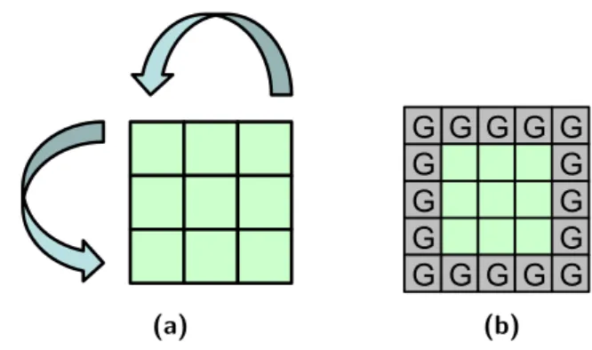
Figure 2.5: Graphical depiction of periodic boundary conditions( Figure 2.5a ) and constant boundary conditions ( Figure 2.5b ) of a 3x3 mesh.

efficient, but it is very often the slowest to converge to a solution [13]. More-over, it is not possible to determine a priori which of the three methods will converge the fastest although heuristics exist. As an example, for problems arising from finite difference approximations, the Red & Black algorithm gives the best results [16].

Consider now a more subtle problem related to numerical convergence. Numerical convergence has to be tested periodically, i.e., at the end of each time step ( or a sequence of time steps ). These tests obviously take some time therefore increasing the total running time of the computations. Even if their contribution can be negligible, they modify the computation structure, reducing its regularity and therefore excluding some optimization techniques. Intuitively, we can understand that if the computation during different time steps is always the same, then we could take advantage of this property, e.g., by collapsing the execution of different time steps.

2.4.2 Boundary Conditions

In the examples in Section 2.3, we selected very simple boundary conditions. Since finite difference methods are used to discretize real world problems, complex boundary conditions may arise. Boundary conditions can be classi-fied in a similar way as stencil computations:

• Constant Boundaries: Boundary values do not change over time. In this case, we have a halo around the boundaries of the grid where values are never updated. These elements are often called ghost cells. • Variable Boundaries: Boundary values change over time. A common

case is periodic boundary conditions where the domain is toroidal; therefore, functional dependencies that exceed the domain boundaries

(32)

are wrapped around the computation domain. As an example, consider a two dimensional domain, where the right neighbour of an element in the right border is the left most element lying in the same horizontal axis.

The case of ghost cells is the easiest to implement and does not affect per-formance. It will be necessary to have slightly bigger data structures in order to contain the ghost cells. Ghost cells will be only read and never updated; therefore, the computation performed for every element is the same. In the case of periodic boundary conditions, additional modulo and conditional op-erations should be introduced in order to distinguish boundary and external elements and to wrap around spatial coordinates on the toroidal domain. In some cases, the handling of boundary conditions can dominate the runtime of a stencil computation[38].

2.4.3 Stencil Coefficients

The matrix presented in equation (2.7) has a very regular structure. However, there are matrices where the non zero elements are not predictable. Thus, it will be necessary to store additional grids of coefficients, increasing the memory transfer per element update. This is true for lattice boltzmann methods (LBM) for computational hydrodynamics[13].

2.4.4 Notable Examples and Conclusions

Other notable examples of widely used stencil computation that are hard to classify are:

• Multigrid methods: Used as PDE solvers, they utilize a hierarchy of discretizations [9]. This approach is based on the fact that the conver-gence of the finite elements methods can be accelerated by varying the domain discretization over time.

• Adaptive Mesh Refinement (AMR) methods: In this class of compu-tations, the discretization is varied over time depending on the actual phenomena that is modelled. As an example consider a physical model with collisions, where we want to dynamically increase the precision of the simulation in the part of the domain where the collision take place. These methods are used when a higher precision on all the domain at all time would make the simulation infeasible[7].

(33)

Notice that AMR methods, although very similar to structured grid com-putations, are dynamic variable stencil computations.

In conclusion, structured grids are a subset of data parallel computations which exhibit a pattern of interaction only between neighbour elements. They usually stem from numerical algorithms for the resolution of partial differen-tial equations, which are in turn at the heart of most simulation codes.

(34)

(35)

Chapter 3 A Hierarchical Model for

Optimization Techniques

In this chapter, we introduce a formal model for optimization methods. The process of concretion from a high level abstraction to an executable pro-gram for stencil computations was presented by Meneghin in his doctoral thesis[31]. Specifically, at the highest level, the stencil computation is ex-pressed in a domain specific language while at the lowest level, an executable file is produced. This process of concretion is performed by a framework for a class of computations.

We claim that optimizations conceptually work at different levels of ab-straction; therefore, they can be added to the concretion hierarchical model. Moreover, their effect can be estimated by defining a cost model at every different level of abstraction, thus providing a tool to analyze program trans-formations. The two biggest difficulties of optimization are:

1. Determining if a transformation is safe. Enforcing a semantic equiva-lence that is too strict will reduce the number of applicable transfor-mations. “Unfortunately, compiler without high level knowledge about the application, can only preserve the semantics of the original algo-rithm” [2]. Therefore, it is necessary to gather domain specific knowl-edge about the application that has to be optimized and render this information usable by a compiler.

2. Determining if a transformation is beneficial for performances.

3. Determining the optimal configuration, i.e. the best parameters, for a large set of different optimizations which have complex interaction patterns.

(36)

The benefits of a framework are obvious for a programmer since it provides high level mechanisms to express a computation. These high level mecha-nisms are implemented in a hierarchical way; therefore, the framework is also extensible. On the other hand, the benefits of optimizations are determined with certainty only by executing the computation. However, it is fundamen-tal to have a structured model to analyze optimizations and estimate their impact using a cost model of the real architecture. Therefore, we claim that by using a single hierarchical model we can represent and analyze both the implementation and the optimization of a class of computations.

3.1 Optimization in a Hierarchical Model

In this section, we introduce the notion of a framework for a generic class of computations[31]. We will assume that we have a domain specific lan-guage for this class of computations. By domain specific lanlan-guage, we refer to a language tailored explicitly to express a subset of all possible computa-tions. Domain specific languages trade generality for expressiveness and for a high level of abstraction, thus resulting in higher productivity[32]. A com-putation expressed with such language features a high degree of abstraction with respect to an executable program described at firmware level. In fact, a high level language has the primary objective of preventing programmers from managing low level mechanisms. However, since the computation is ex-ecuted on a real architecture, there is a gap between the level of abstraction desired by a programmer and the execution of the computation. A frame-work fills this gap between the high level representation and the firmware level executable by implementing the concretion process. This process con-sists in the transformation of a program described at the highest level into its equivalent version at the lowest level. The process is structured in a hierar-chical way, meaning that it is defined on multiple steps. Every level i in this process has a set of instruction (or mechanisms) Ii and a specific language Li. Moreover, every mechanism of a level i is implemented at a lower level j using mechanisms defined in the language Lj.

Now, we have to define a concretion step between two levels.

Definition 3.1 (Concretion Function). Given two adjacent levels of abstrac-tion, the concretion function Ci

j is a mapping from the higher level i to the lower level j which is always defined for every semantically correct program. We are implicitly stating that there always exists a naive way to translate a program from a high level of abstraction down to an executable one. If we only consider the definition of the concretion function and define the language

(37)

Chapter 3. A Hierarchical Model for Optimization Techniques

of every level, we have a model for the concretion of a class of computations. However, we enrich this model in order to account for optimizations. Intu-itively, an optimization transforms an input program into an equivalent one, which performs better on a given architecture. Aho et al.[2] introduce the concept of optimization as “Elimination of unnecessary instructions in object code, or the replacement of one sequence of instructions by a faster sequence of instructions that does the same thing”. Although it is very clear, this is not a formal definition.

Definition 3.2 (Program Transformation). Let the space of well formed pro-grams at level i be L∗_i. A program transformation is a function of L∗_i in itself.

Therefore, given a program a ∈ L∗

i, a transformed program b ∈ L∗i is produced. Notice that a transformation is defined on a specific level. It is obvious that a program transformation is relevant only if it preserves the meaning of the program; in that case, the transformation is legal (or safe). The explicit definition of legal transformation was debated extensively in the compiler research field. Bacon et al.[5] give many possible definitions of a legal transformation and conclude that the following is the most reasonable: “A transformation is legal if the original and the transformed programs pro-duce exactly the same output for all identical executions”. However, we will provide a more abstract definition that better suits our needs. More pre-cisely, in order to formally define a legal transformation, we need to define the concept of equivalence of two programs.

Definition 3.3 (Equivalence). For every level i, there exists a formal seman-tic associated to every well formed program expressed in Li. Two programs a and b will be equivalent at level i if their semantic is equal: JaKi = JbKi. Therefore, the space of well formed programs at level i will be partitioned into disjoint groups of equivalent programs.

Now we can define:

Definition 3.4 (Legal Transformation). A transformation f defined at level i is legal if ∀a ∈ L∗

i f (a) = b =⇒JaKi =JbKi

In other words, a transformation is legal if for every input program, it produces an equivalent one. There could be an infinite number of legal transformation which can be trivially obtained from a given input program a. As an example, consider a sample piece of code defined in a general purpose language:

B[i , j ] = A[i,j ] + 1

(38)

An equivalent program is:

B[i , j ] = A[i,j ] +3 −2

The semantic of the right hand side of both statements is obviously the same and countless other legal transformation can be made in a similar trivial way. Until now, we have only defined a program transformation and a legal trans-formation. An optimization is a legal transformation which introduces some benefits in terms of performance. Performance is evident when executing the application on a real architecture. Therefore, we need to formally introduce the concept of performance in our model. In order to do so, we assign a cost model to every level.

Definition 3.5 (Cost Model). Given the space L∗_i of well formed programs at level i, cost model _Ci for level i is a function of L∗i to R+.

This is a very general definition because it states that for every level, there exists a function that associates every program to its cost, which cannot be negative. Since our model is hierarchical, the cost model should also be hierarchical. Therefore, the cost model at the highest level features a high level of abstraction and it does not consider peculiarities of specific architectures. On the other hand, the cost model of lower levels should be closer to the actual execution of the application on the given architecture. Next, we formally define an optimization.

Definition 3.6 (Optimization). Given a hierarchical model which corre-sponds to the execution of a computation on a target architecture, a legal transformation f , defined at level i, is an optimization if _∃P1 ∈ L∗i. f (P1) = P2 and at an underlying level j ≤ i, the cost of the transformed program Cj(P2) is less than the cost of the original program Cj(P1)1.

In other words, an optimization for a program corresponds to the applica-tion of a legal transformaapplica-tion such that the cost of the transformed program is lower at an underlying (or at the same) level of abstraction. We are not imposing that the cost should be lower at the same level of abstraction where the transformation is applied. This is because the cost model at an higher level might be too abstract to capture the advantage of the optimization ( this is the case of many optimizations described in Chapter 4). Notice that we are also not implying that the cost of the transformed will be lower at the firmware level, where it corresponds to the actual completion time of the computation. Otherwise, we would have that an optimization, in order

1_{When considering the cost of a program C}

j(P1) where P1 is defined at a higher level

(39)

Chapter 3. A Hierarchical Model for Optimization Techniques

to be labelled so, has to increase performances on any possible real archi-tecture which is generally infeasible. The extreme consequence is that we could only define optimizations at the firmware level (therefore only for a specific architectures). Instead, we want to define and analyze optimizations using abstractions that are oblivious to architecture peculiarities. It would be compiler’s responsibility to decide when to apply a given optimization after knowing the real architecture where the program has to be executed.

This definition of optimization in a hierarchical model, although fairly ab-stract, expounds many real practices in compilation techniques. The equiva-lence classes of a program at a given level correspond to the space of possible optimizations (optimization space). A heuristic serves to prune this space and eliminate choices that are known to be inefficient. After space pruning, the compiler will make a choice among all candidate programs. Notice that this type of optimization problems are usually NP, e.g., selecting the best partitioning[15]. Defining the process on multiple levels reflects the fact that optimizations works at different levels of abstraction. Therefore, an opti-mization working at higher level of abstraction, where the semantics of the language is as close as possible to the intended semantics of the program, will manage different mechanisms with respect to a peephole optimization2 working on the object code of the application.

3.2 The Reference Architecture

In this section, we introduce the notion of a framework for the class of stencil computations developed in[31]. Similarly to Section 3.1, we will assume that we have a domain specific language[32] for the class of stencil computations. We will use these computations as an example throughout all this thesis, but note that the formalization presented in the previous section is valid for any generic computation. A stencil representation, defined with a domain specific language, features a high degree of abstraction with respect to an executable program described at firmware level. The model presented in this section will give an idea of the whole process of concretion. In [31], the concretion process was defined on four separate levels:

1. Functional Dependencies.

2. Partition Level.

2_{In compiler theory, peephole optimization is a kind of optimization performed over}

a very small set of instructions in a segment of generated code, e.g., removing duplicate instructions.

(40)

3. Concurrent Level. 4. Firmware Level. Assembler: LOAD STORE DMA.. Processes and Chennels: send-receive Partition Strategy, Partition Regions System Levels System Abstractions Steps, Shape, Application Points C oncr etiz ation High Abstraction Degree Low Abstraction Degree P rogrammers Framework Support Functional Dependencies Partition Dependencies Concurrent Language Assembler - Firmware

Figure 3.1: Framework for stencil computations as presented in [31].

I The stencil computation is defined at the highest level of Functional Dependencies.

II The stencil computation, defined at the functional dependencies level is then translated in the underlying Partition Level where functional dependencies become dependencies among partitions.

III At the Concurrent Level, the partitions are associated to different processes and the dependencies between partition become communica-tions among processes. Therefore, we assume that a message passage paradigm is used.

IV Finally, we compile an executable program by means of a standard com-piler.

We briefly explain these steps showing the concretion process for a struc-tured grid computation: the Laplace operator of Figure 2.3. At every step, we will indicate language, equivalence class, and cost model of every level.

Optimization Techniques for Stencil Data Parallel Programs: Methodologies and Applications

University of Pisa and Scuola Superiore

Sant’Anna

Master Degree in Computer Science and Networking

Corso di Laurea Magistrale in Informatica e Networking

Master Thesis

Optimization Techniques for

Stencil Data Parallel Programs:

Methodologies and Applications

Candidate

Supervisor

Andrea Lottarini

Prof. Marco Vanneschi

Contents

List of Figures

Listings

Chapter 1

Introduction

1.1

Structured Grid Computations

1.2

Thesis Outline

Chapter 2

Data Parallel with Stencil

Computations

2.1

Map Computations

2.2

Data Parallel with Stencil Computations

2.2.1

Classification of Stencil Computations

2.3

Structured Grids in the Real World

2.3.1

Finite Difference Method

2.3.2

Discretization of Partial Differential Equations

2.3.3

Iterative Methods to Solve PDE

2.3.4

Heat Equation

2.4

Properties of Structured Grid

Computa-tions

2.4.1

Convergence

16

G G G G

G

G

G

G

G

G

G G G G G

(a)

A 2D grid with ghost

cells for storing

boundary conditions.

(b)

A 2D grid with periodic

boundary conditions

and no extra cells.

G

Figure 2.5: In (a), we show a 3

×3 grid with surrounding ghost cells (marked with a

“G”) that are used to store boundary conditions. In (b), we show a 3

×3 grid which

does not require ghost cells because it has periodic boundary conditions.

Constant Boundaries

There are two main types of constant boundary conditions. In the first case, the

points along the boundary do not change with time, but do change depending on

position. In this case, we can use ghost cells (like in Figure 2.5(a)) to store these

values before any stencil computations begin. Once the ghost cells are initialized,

they do not need to be altered for the rest of the problem. In this thesis, all three

3D stencil kernels have this type of boundary condition. However, the ghost cells

consume a non-trivial amount of memory for 3D grids. Suppose that we have an N

3

grid that is surrounded by ghost cells. Then, the resulting grid has (N + 2)

3

_{×3 grid with surrounding ghost cells (marked with a}

_{×3 grid which}