Scuola di Ingegneria Industriale e dell'Informazione
Corso di Laurea Magistrale in Ingegneria Elettrica
A Method to Classify Substation Load Profiles Based
on PCA
Relatore: Prof. Alberto Berizzi
Correlatore: Dott. Alessandro Bosisio
Tesi di Laurea Magistrale di:
Tianxing Qi
Matr. 10534003
INDEX
ABSTRACT ... 1
1 INTRODUCTION ... 3
1.1 Research Background ... 3
1.2 Research status ... 5
1.3 Thesis content and outline ... 6
2 BASIC CONCEPTS OF LOAD PROFILE CLASSIFYING ... 8
2.1 Load classification in power system ... 8
2.2 Load data preprocessing ... 12
2.2.1 Bad data processing ... 13
2.2.2 Normalization ... 14
2.2.3 Missing value processing ... 16
2.2.4 Outliers processing ... 24
2.3 Summary ... 26
3 BASIC CONCEPT OF PCA ... 27
3.1 Introduction of PCA ... 27
3.2 Basic idea ... 27
3.2.1 Goal ... 28
3.2.2 Definition and property ... 28
3.3 Data process ... 31
3.3.1 Data requirements ... 31
3.3.2 Data standardization ... 33
3.4 Summary ... 34
4 THE LOAD CLUSTERING MODEL BASED ON PCA ... 36
4.1 The load clustering model based on PCA ... 36
4.2 Loading raw load data from the database ... 38
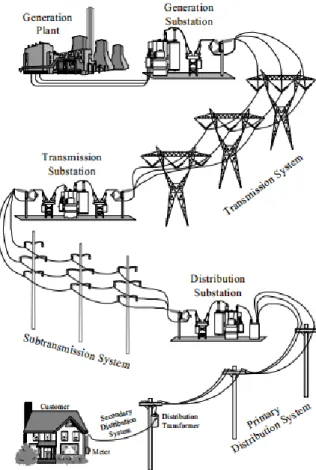
4.2.1 T&D system in Italy ... 38
4.2.2 Database in UNARETI company ... 40
4.2.3 Refined database building ... 44
4.3 Load data preparation ... 45
4.3.1 Defining and deleting bad data ... 45
4.3.2 Data normalization ... 47
4.3.3 Data interpolation ... 48
4.3.4 Outliers processing ... 49
4.4 PCA method in load profile ... 51
4.4.1 PCA in load profiile ... 51
4.4.2 The process to apply PCA ... 51
4.5 Load profile classification and application ... 53
4.6 Summary ... 54
5 RESULT OF THE PCA ON LOAD PROFILES ... 56
5.1 Analysis of PCA components ... 56
5.1.2 PCA main components ... 56
5.1.3 The load properties of main components ... 59
5.1.4 Brief summary ... 63
5.2 Result of load profile classification ... 63
5.2.1 Classification result ... 63
5.2.2 Geographic proof ... 65
5.3 Load profile classification by the daily peak load ... 68
5.4 Summary ... 70
6 CONCLUSIONS ... 71
INDEX OF FIGURE
Figure 2.1: Example of the piecewise constant interpolation ... 17
Figure 2.2: Example of the linear interpolation ... 18
Figure 2.3: Example of Piecewise Cubic Hermite Data Interpolation ... 21
Figure 2.4: The example of boundary problem with PCHIP method ... 22
Figure 2.5: The PCHIP plus ARMA interpolation method process ... 24
Figure 2.6: The example of PCHIP plus ARMA interpolation in boader ... 24
Figure 2.7: The possibility distribution for normal distributed data... 26
Figure 3.1: The corresponding PCA analysis process algorithm ... 31
Figure 3.2: The PCA application situations... 33
Figure 3.3: PCA concept clarification ... 35
Figure 4.1: The clustering stages of the load profiles... 37
Figure 4.2: The power delivery system ... 38
Figure 4.3: The continous lacking substations ... 47
Figure 4.4: The PCHIP method compared with PCHIP+ARMA method ... 49
Figure 4.5: The process of filling the outliers ... 50
Figure 4.6: Example of an outlier fixing ... 51
Figure 4.7: The process of PCA in load profile analysis ... 52
Figure 4.8: The classification model ... 54
Figure 5.2: Coefficients of the first main component ... 57
Figure 5.3: The coefficients of the second main component ... 58
Figure 5.4: Average daily temperature in Milan ... 58
Figure 5.5: The coefficients of the third main component ... 58
Figure 5.6: Coefficients of the third main component in Feburary ... 59
Figure 5.7: The score of all the substations in couple ... 60
Figure 5.8: Load profile of No.809 and No.496 substations ... 60
Figure 5.10: The load profile of No.156 and No.450 substations ... 61
Figure 5.11: The load profile of No.411 and No.758 substations ... 62
Figure 5.12: The two week load profile of No.411 and No.758 substations ... 62
Figure 5.13: Scatter graph of three components ... 64
Figure 5.14: Octants classification method ... 64
Figure 5.15: Load classifications distributions ... 66
Figure 5.16: Different load classifications in in google map ... 66
Figure 5.17: Type 1 substation in google map ... 67
Figure 5.18: Type 2 substation in google map ... 67
Figure 5.19: Type 7 substation in google map ... 68
Figure 5.20: Type 8 substation in google map ... 68
INDEX OF TABLE
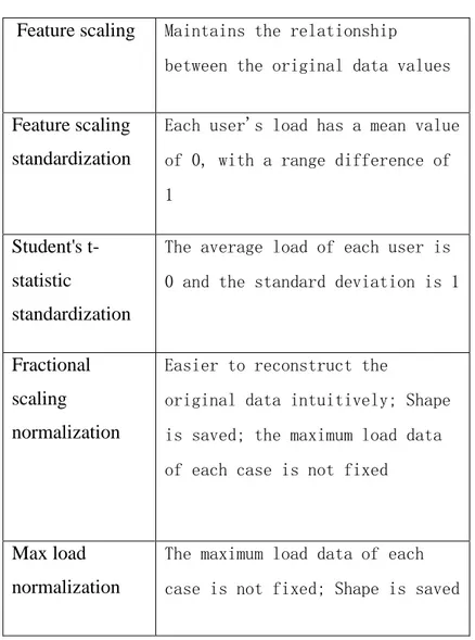
Table 2.1 Typical normalization methods ... 16
Table 2.2 Value table of unknown function f(x) ... 17
Table 4.1 The original daily load profile database ... 40
Table 4.2 The original coordinates database ... 41
Table 4.3 The original LV customer information database ... 42
Table 4.4 The original overload number information database... 43
Table 4.5 The refined database ... 44
Table 4.6 The typical interpolation methods comparation ... 47
Table 4.7 The detail database scale ... 51
Table 5.1 The explain matrix of the daily load... 56
ABSTRACT
Abstract in italiano
Questa tesi tratta un metodo per classificare i profili di carico delle cabine secondarie MT, basato sull‟analisi delle componenti principali (PCA).
La procedura di classificazione si articola su cinque passaggi: 1) Caricamento dei profili di carico: in questa fase la base dati viene omogeneizzata e semplificata. 2) Preparazione dei dati: questa fase include quattro processi: identificazione e ed eliminazione delle serie non valide, normalizzazione dei dati, interpolazione dei dati e rilevamento dei valori anomali. Una combinazione di Piecewise Cubic Hermite Interpolating Polynomial (PCHIP) e Autoregressive Moving-Average (ARMA) viene applicato per l‟interpolazione dei dati agli estremi della serie. 3) Semplificazione dei dati tramite PCA. La PCA che viene utilizzata per estrarre le componenti principali, al fine di ridurre la dimensione dati base. 4) Classificazione dei profili di carico: le cabine secondarie vengono classificate in 8 gruppi sulla base delle prime 3 componenti principali 5) Interpretazione dei risultati.
Analizzando i risultati della classificazione, si può ipotizzare che: 1) Le prime 3 componenti principali rappresentano: il fattore presenza/assenza di attivita, il fattore di condizionamento estivo e il fattore carico feriale/festivo. 2) Definendo 8 tipologie di profilo, solo quattro risultano significative.
I clienti di “tipo 1” sono caratterizzati da una uniforme attivita durante tutto l‟anno, forte utilizzo del condizionamento estivo, limitata differenza tra carico feriale e festivo; i clienti di “tipo 2” sono caratterizzati da una riduzione dell‟attivita durante il periodo agostano, forte utilizzo del condizionamento estivo, limitata differenza tra carico feriale e festivo; i clienti di “tipo 3” catatterizzati da una riduzione dell‟attivita durante il periodo agostano, basso utilizo del condizionamento estivo, sensibile differenza tra carico feriale e festivo; i clienti di “tipo 4” caratterizzati da una uniforme attivita durante tutto l‟anno, basso utilizzo del condizionamento estivo, sensibile differenza tra carico feriale e festive.
Abstract in inglese
This thesis is about a method to classify MV/LV substation load profiles based on principle component analysis (PCA) method, considering the real daily load data from the UNARETI company in Milan. The classification model includes five steps: 1) Loading raw load profiles: in this step time series are refined and simplified. 2) Data preparation: this step includes four processes: defining and deleting the bad data, normalizing data, the data interpolation and outlier detecting. A method that combines PCHIP and ARMA is applied to deal with the boundary issues. 3) Data simplifying with PCA method: PCA method is used to extract the main components, in order to decrease the dimension of the data. 4) Load profile classification: MV/LV substations are classified in 8 groups based on the first 3 components. 5) Result applications. By analyzing the load customers classifying in Milan, it can be concluded that 1) The main 3 components of daily load profile are: the activity factor, the air conditioner factor and the holiday factor. 2) After the classification, 8 types of substations have been identified but only four result to be common. Type 1 customers have the character of uniform activities, high airconditioner occupancy, low holiday differences, for example commercial center; Type 2 customers have the character of non-uniform activities, high airconditioner occupancy, low holiday differences; Type 3 customers have the character of non-uniform activities, low airconditioner occupancy, high holiday differences; Type 4 customers have the character of uniform activities, low airconditioner occupancy, high holiday differences.
Keyword: load classification; principle components analysis; data processing; load profile
1 INTRODUCTION
Load classification has always been the basis of power system planning, peak management, flexible electricity price, and load forecasting. Good load classification methods can provide correct basis and guidance for system planning and peak load management. Therefore, a method of load classification is studied in this thesis. Based on real data, this method is applied to the load classification of the Milano distribution, and the load characteristics of the power grid are analyzed in detail.
1.1 Research Background
Nowadays, the load is growing rapidly, but the analysis of power load characteristics is still at a relatively less studied stage, mainly reflected in the following aspects:
(1) The models and data required for the analysis of load characteristics are dispersed in multiple production and management systems. The underlying data has not been integrated and unified data management and analysis cannot be performed;
(2) There are many types of users in the power system, and various types of users exhibit different load characteristics. Currently, there is a lack of a scientific and effective load classification method and a comprehensive load characteristic index system that meets the actual conditions of the power grid.
(3) There are many kinds of influencing factors for the classification of load characteristics, and the influences for each kind are different. At present, there is no in-depth and systematic analysis for the factors affecting the change of load characteristics and the degree of influence.
(4) The research on the classification load characteristics is not thorough, and its rules are not accurately studied. An effective statistics and analysis system cannot be formed. The effective technical support and guidance can not be provided for load forecasting, power grid planning, economic dispatch and electricity market.
The above problems have restricted the further improvement of the load management and application in the power grid, and lead to the difficulties to adapt to the requirements of refined management and technical progress of the power grid. At present, there are
many researches on power grid load forecasting, but there are relatively few studies on load classification. Load classification is the basis of load forecasting. Through the analysis of load characteristics and load classification, it is very important to understand the changes and trends of power grid load. It is necessary, therefore, to study accurate and appropriate load classification method is of great significance.
In the long run, accurate load classification methods are not only beneficial to the power system, but also beneficial to users, and are specifically expressed in the following aspects:
(1) Beneficial to power system
The scientific and accurate load classification method can save the country‟s infrastructure investment in the power industry, improve the thermal efficiency of power generation equipment, reduce fuel consumption, reduce the cost of power generation, increase the safety and stability of power system operation, improve the quality of power supply, and is conducive to the overhaul of power equipment. At the same time, it is an important basis for power planning, production, and operation. It is also an important reference for formulating relevant policies. It provides technical guidelines for the production and operation in power grids, power grid planning, the power grids accurate management, and innovative creation work. To meet the requirements of the development and improvement of the economy, power companies must understand the market, rely on the market, open up markets, and scientifically accurate load classification to optimize the planning and operation of the power grid, improve the quality of customer service, and ensure the safety, economy, quality and environmental protection of the power grid.
(2) Beneficial to the users
The ultimate beneficiaries should be mostly users. Since the country‟s investment in user equipment can be saved, shaving peak load and filling valley load, where electricity consumption during peak hours is led to the valley hours, can reduce electricity bills, which in turn reduces production costs and benefit the people in urban and rural residents. As a result of the measures taken, employees of factories and factories have taken a break from work and staggered work shift times, so that the load of service industries such as local transportation, water supply and gas supply and so on can be balanced.
1.2 Research status
With the development of smart grid, more and more smart meters are installed into distribution networks [1]. Consumption behaviors of customers are known through load curves data collected from smart meters. Clustering technology is very useful for data mining in smart gird. In competitive electricity market with severe uncertainties, performing effective customer classification according to customers' electrical behavior is important for setting up new tariff offers [2].
The load classification is to separate enormous load profiles into several typical clusters.[3] In recent years, researchers have proposed a variety of clustering methods. Various methods for clustering load curves have been used in the load clustering in recent years. such as K-means[4]-[5], fuzzy c-means(FCM) [6]-[8], hierarchical methods[9], [10], self-organizing map (SOM) [11], support vector machine (SVM) [12], [13], subspace projection Method [14].
In the meanwhile, there are some papers combining some methods together. In [15], a method combine with hierarchical and fuzzy-c mean was introduced. [16] proposes a two-stage clustering algorithm combining supervised learning methods to classify electric customer.
With the development of data mining technologies, some new clustering methods have emerged for electricity consumption patterns classification. In paper [17], they built a prediction model to identify the customers who would most likely respond to the prospective offering of the company. Thus in [18], the extreme learning machine method is used to analyze the nontechnical loss to classify the customers.
However, in the data mining technologies, instead of improving the method of clustering, decreasing the dimension of the data and extract the main features of the load profile can be another important method to cluster. In [19], a statistical analysis of end-users‟ historical consumption is conducted to better capture their consumption regularity. With the features captured, it is easier to classify the customers. [20] focus on the description of the construction and implementation of the recognition of customers' risk preference model. Consider the following information: customer consignment streamline data, customer exchange streamline data, customer fund streamline data, and so on. Using
PCA, two important indicators, behavioral characteristics and risk preferences of the customers, are selected, with which the construction of the customer classification model is built with K-means clustering algorithm.
1.3 Thesis content and outline
According to the achievements and existing problems in the field of power load classification, this thesis analyzes daily load data of more than 4000 MV/LV substations in Milano. A methodology to classify distribution load profiles based on PCA method is put forward. Based on the basic theory of classification of load characteristics, a procedure has been defined as follow:
(1) Select the substation daily peak load curve (366 values, in the year 2016) as the load feature vector of the power system user, and deal with the data in three steps: defining bad data, data interpolation and dealing with outliers;
(2) PCA (Principal Component Analysis) is used to analyze the load eigenvectors of the substations, the principal components are extracted, the dimension of the data set is reduced, and each principal component is analyzed.
(3) According to the results of the principal component analysis, MV/LV substations load profile are classified, and combined with geographical information, a set of load types are defined and classified.
The thesis is organized as follows:
(1) The basic concepts and theories of load classification. This chapter mainly introduces three aspects: the load characteristics and type of power system, the extraction and preprocessing of load data, and the basic load classification method.
(2) Basic concepts of load profile classifying. This chapter mainly introduces the basic concept of load classification. On one side, it introduced the profile classification already known and the need to produce a new load classification. On another side, the load data preprocessing, which is one of the most important task in load classification, is studied in four aspects, that is bad data processing, load curve normalization, missing value processing, and outlier processing.
(3) The basic concepts and theories of principal component analysis. This chapter introduced the basic principles and properties of principal component analysis, and lists the basic steps of principal component analysis. In addition, two important points of principal component analysis are discussed in the end of the chapter: data requirements and the data standardization.
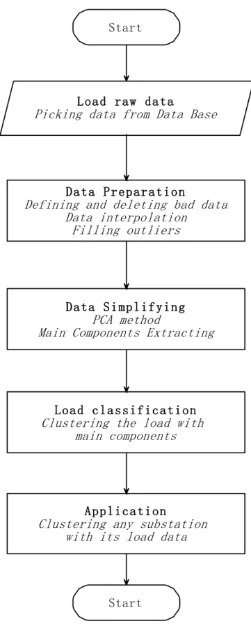
(4) The load classifying model based on PCA method. This chapter mainly introduced the five steps of the procedure, that is: loading raw load data from the database, load data preparation, data simplifying with PCA method, load profile classification and applications. Based on the real data from the Milano distribution network, among all the five steps, the loading of raw data is mainly introduced.
(5) The result analysis. In this chapter, at first, the result of PCA is given. And after the analysis, the main components are settled down. Then, with the result of PCA, the classification of the substations is given, together with the meaning of each classification.
2 BASIC CONCEPTS OF LOAD PROFILE
CLASSIFYING
With the in-depth development of the electricity market and the extensive application of DSM technology, the load classification of power systems has become a very important basic work, such as load pricing, load forecasting, system planning, and load modeling. To complete all of the work needs to have a scientific and accurate classification of the type of load. Therefore, the in-depth study of methods and applications of power system load classification helps to timely master the changes in the law and trends of power load, and it helps to the scientific management of electricity load, which is beneficial to planning for the development of electricity use. Therefore, it has important theoretical and practical significance.
2.1 Load classification in power system
The basic task of the power system is to provide uninterrupted high-quality electrical power to meet the needs of various types of loads. Normally, the load is the workload that a transformer substation or a grid is responsible for at a certain moment. For the user, the power load refers to the sum of the power consumed by all the user's devices connected to the power grid at a certain moment.
The power system load characteristics, whether for the system planning and design, or the optimized safety operation, are extremely important. Therefore, research on load characteristics is an important task of the power system. Research on load forecasting, load classification, load pricing, load demand side management and load modeling has become an important research area in the modern power market environment, and it is also an important content in the field of power system automation research.
The actual power system has a variety of loads, and the total system load is a sum of various types of loads. Therefore, for the actual power system, all types of loads should have a formal and accurate classification, so that the same type of load has the same or similar characteristics, thereby simplifying or reducing the difficulty and complexity of load management.
In general, the load can be divided into urban civilian loads, commercial loads, rural loads, industrial loads, and other loads. The urban civilian load mainly refers to the urban household load, and the commercial load and industrial load are the load of commercial and industrial services. The rural load refers to the load of all rural areas (including the rural civilian load, production, irrigation and commercial electricity, etc.), while other loads include municipal electricity (e.g. street lighting), utilities, government offices, railways and trams, military and others. According to different standards, different types of loads can be divided:
1. Divided by physical performance
According to the physical performance of the load can be divided into active load and reactive load.
(1) Active load: It is the energy that is converted into other forms of energy and is actually consumed in electrical equipment. The unit of calculation is kW (kilowatts).
(2) Reactive power load: In the process of power transmission and conversion, it is necessary to establish the power consumed by magnetic fields (such as transformers, motors, etc.) and electric fields (such as capacitive field energy). It only completes the conversion of electromagnetic energy and does not do work. In this sense, it is called "reactive power" and the unit of calculation is l kvar.
2. Divided by electrical energy
According to the production, supply, and production of electricity, the load can be divided into generation load, power supply load, and electricity load.
(1) Power generation load: It refers to the power load that the power plant supplys to the power grid, plus the power load consumed by the power plant itself at the same time, and the unit is kW.
(2) Power supply load: It refers to the sum of the power generation load of each power plant in the power supply area, minus the power load consumed by the power plant itself, plus the load inputted from other power supply area, minus the load absorbed by the other power supply area, unit kW.
(3) Customer load: It refers to power supply load in the area minus the loss in the line and the transformer. The unit of calculation is kW.
3. Divided by time scale
The load can be divided into yearly load, monthly load, daily load and hourly load .
4. Divided by requirements for reliability of power supply
According to the nature of the electricity load and the different requirements for the reliability of the power supply, the load can be divided into level-one load, level-two load and level-three load.
(1) Level-one load: The event of a power outage in this load will result in personal injury or death, or political, military, and economically significant losses, such as an accident that endangers personal safety, causes unrecoverable damage or disorder to key equipment in industrial production, resulting in major losses in the national economy. The loads of important military facilities, hospitals, airports and other places generally belong to this class of loads.
(2) Level-two load: When the blackout occurs in this load, it will result in production cuts, work stoppages, traffic congestion in some areas, and troubles in the normal activities for a large number of residents in cities. For instance, the load of residents and factories in large and medium-sized cities generally are always classified into level-two load.
(3) Level-three load: It is general loads other than level-one and level-two loads. The loss caused by the interruption of such loads is not significant. Such as the factory's ancillary workshops, small towns and rural public loads, etc. are often classified as such loads.
5. The international general classification of electricity load
According to the international general classification of the power load, the power load can be divided as follows:
(1) Agriculture, forestry, animal husbandry, fishery and water conservancy. Rural irrigation, agricultural side production, agriculture, forestry, animal husbandry, fisheries, water conservancy and other kinds of load are included.
(2) Industry. A variety of mine industries, manufacturing and other kinds of load are included.
(3) Geological survey and exploration industry. (4) Construction industry.
(5) Transportation, post and telecommunications. Loads in road and railway station, ship terminals, airport, pipeline transportation, electrified railway and post and telecommunication are included.
(6) Commercial, public catering, material supply and warehousing, various stores, catering, material supply units, and warehouse loads.
(7) Other institutions. The load in the city's public transport, street lighting, art and sports institutions, national party and government agencies, various social groups, welfare services, scientific research institutions and other units is included.
(8) Urban and rural household electricity.
Although load in the power system can be divided according to the above criteria, such classification is not strict and accurate. In the actual classification, it may happen that the actual load is reduced to what kind of dispute.
In this case, it is generally determined by the power supply department itself. Therefore, in some power supply departments, each of them may have its own more load classification list in detail in order to prepare for load classification. However, there are still some problems in the practical application of the load classification method adopted by the above power supply department:
(1) Users in the same work field may have different load characteristics.
At present, the power supply department classifies the power system user load, most of which is based on the industry to which the user load belongs and the economic activity characteristics of the user. However, as the composition of the user's load devices becomes more and more complex and people's production and lifestyle changes, the user's load characteristics in the same industry are not exactly the same, and their load curves may have large differences.
(2) It cannot reflect changes and differences in the power grid.
With the development of economy and society, there will be some new types of user loads in the power grid, and these types of user loads may have large differences from the already defined types of user loads. Therefore, it is necessary to reconsider the type and definition. And there are also certain differences in the load composition between the power grids in different regions. The load types of the power grids should be divided according to the actual situation.
(3) Inaccurate classification affects the further application on this basis.
The traditional load classification method does not fully consider the actual characteristics and rules of the customer load, lacks theoretical basis. And it reduces the accuracy and rationality of the classification result, affecting some applications. For example, it reduces the accuracy of the classification load forecasting, which causes the unreasonable electricity price policy and so on.
Therefore, in order to solve the above problems, it is necessary to study a scientific and accurate load classification method to provide powerful reference and basis for load classification based on which new applications can be applied in the power supply department.
2.2 Load data preprocessing
It is often said that 80% of data analysis is spent on the process of cleaning and preparing the data. Data preparation is not just a first step, but must be repeated many times over the course of analysis as new problems come to light or new data is collected. Despite the amount of time it takes, there has been surprisingly little research on how to clean data well. Part of the challenge is the breadth of activities it encompasses: from outlier checking, to date parsing, to missing value imputation.
The load database is extremely large, and the database can be easily affected by noise, lost data, and inconsistent data. Low quality load data will lead to low accuracy of classification results, so data preprocessing is an important first step in load classification. Data preprocessing usually includes four aspects: bad data processing, load curve normalization, missing value processing, and outlier processing.
In power systems, almost all research on loads is based on raw data. Therefore, the accuracy of the research results is determined by the correctness of the original data. The raw data is usually directly derived from the real-time data collected in the EMS/SCADA system. Due to the dynamic data acquisition, there are sometimes channel failures, congestion, and other phenomena. In addition, the interruption of the data acquisition program can also cause errors in the original data. At the same time, according to the needs of the classification method used, the data needs to be normalized and other processing. Therefore, before applying the method of this thesis to study the system load classification, we need to preprocess the sample data from the following aspects.
2.2.1 Bad data processing
Bad data can be defined in just a few general classifications. The vast majority of data quality professionals would break data quality issues in these terms:
1. Incomplete data: A data record that is missing the necessary values that render the
record at least partially useless.
2. Invalid data: A data record that is complete, but has values that are not within
pre-established parameters.
3. Inconsistent data: Data that is not entered in the same way as the other data
records.
4. Unique data: A data record unlike any other previously measured data record. 5. Legacy Data: Defining data as too old can also be very important in order to utilize
data that is still relevant to the organization, and excluding data that was collected before certain variables were established.
There are many causes of bad data, which may be determined by the inherent characteristics of the data generation mechanism, or may be due to imperfect data acquisition equipment, data transmission errors, data loss and other human controllable factors. Bad data includes missing values, 0 values, and straight line load values. Bad data identification includes physical identification and statistical identification.
The physical identification method is based on people's experience in identifying bad data. The statistical identification method is to give a confidence probability and determine
a confidence threshold. Any error that exceeds this threshold is considered not to belong to the random error range, and it is considered as a method of rejecting bad data. The physical identification is usually used in bad load data detection.
2.2.2 Normalization
The user load data obtained through the power system load measurement device will have a large difference in the value range, and these differences will have a great impact on the classification result. Therefore, sample data should be normalized before classification to eliminate the influence of these differences.
There are several ways to normalize data. Here introduces five normalization methods: To make it simple, the original user load is presented as
X
( ,
x x
1 2,...,
x
n)
.1. Feature scaling
The user data is normalized according to Equation (2-1), and the value
x
i is mapped tox
i
in the interval [a,b]. The feature scaling maintains the relationship between the original data values.min( )
(
)
1, 2,...,
max( )
min( )
i ix
X
x
b a
a
i
n
X
X
(2-1) 1 2max( )
X
max( ,
x x
,...,
x
n)
(2-2) 1 2min( )
X
min( ,
x x
,...,
x
n)
(2-3) Normally, a = 0 and b = 1, so the normalized data range is between 0-1.2. Feature scaling standardization
After the feature scaling standardization, each user's load has a mean value of 0, with a range difference of 1, and
x
i
1
. So the error can be reduced in the PCA.1
1
n j jX
x
n
(2-4)1, 2,...,
max(
)
min(
)
i ix
X
x
i
n
X
X
(2-5)3. Student's t-statistic standardization
After the student's t-statistic standardization, the average load of each user is 0 and the standard deviation is 1. The equation shown below is the calculation:
,
1, 2,...,
i ix
X
x
i
n
s
(2-6) 2 11
(
)
1
n i is
x
X
n
(2-7)It is always used to normalize residuals when population parameters are unknown
4. Fractional scaling normalization
The decimal scaling is normalized by moving the decimal places in
x
i. The number of decimal places to move depends on the maximum absolute value ofx
i. The formula is as follows, where i is the smallest integer which makesmax(
x
i
) 1
.10
i i i
x
x
(2-8)In this method, all the load can be restricted to [0,1]. Due to the factor is the base of 10, it is easier to reconstruct the original data intuitively. And the shape of data is saved. But it has a problem that the maximum load data of each case is not fixed.
5. Max load normalization
The max load normalization is normalized by dividing the maximum load. This normalization is based on the fact that all the load data are larger than zero. This kind of normalization is simple, and the load shape can be reserved.
,
1, 2,...,
max( )
i ix
x
i
n
X
(2-9)Table 2.1 Typical normalization methods Feature scaling Maintains the relationship
between the original data values
Feature scaling standardization
Each user's load has a mean value of 0, with a range difference of 1
Student's t-statistic
standardization
The average load of each user is 0 and the standard deviation is 1
Fractional scaling normalization
Easier to reconstruct the
original data intuitively; Shape is saved; the maximum load data of each case is not fixed
Max load normalization
The maximum load data of each case is not fixed; Shape is saved
2.2.3 Missing value processing
During the data collection process, due to equipment or machinery, some missing values can be generated. Dealing with missing values of non-bad data, interpolation is an effective method. In the field of numerical analysis, interpolation is a method of constructing new data points within the range of a discrete set of known data points.
A closely related problem is the approximation of a complicated function by a simple function. Suppose the formula for some given function is known, but too complicated to evaluate efficiently. A few data points from the original function can be interpolated to produce a simpler function which is still fairly close to the original. The resulting gain in simplicity may outweigh the loss from interpolation error.
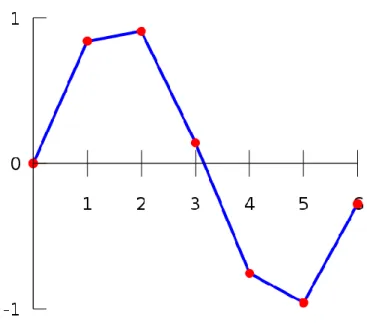
Given the values of an unknown function f(x) in table 2.2, there are some methods that can be used to interpolate the missing data:
Table 2.2 Value table of unknown function f(x) x f(x) 0 0 1 0.8415 2 0.9093 3 0.1411 4 -0.7568 5 -0.9589 6 -0.2794
1. Piecewise constant interpolation
The simplest interpolation method is to locate the nearest data value, and assign the same value. In simple problems, this method is unlikely to be used, as linear interpolation is almost as easy, but in higher-dimensional multivariate interpolation, this could be a favorable choice for its speed and simplicity.
Figure 2.1: Example of the piecewise constant interpolation
Another simple method is linear interpolation (sometimes known as lerp). Consider the above example of estimating f(2.5). Since 2.5 is midway between 2 and 3, it is reasonable to take f(2.5) midway between f(2) = 0.9093 and f(3) = 0.1411, which yields 0.5252.
Figure 2.2: Example of the linear interpolation
Generally, linear interpolation takes two data points, say
(
x y
a,
a)
and(
x y
b,
b)
, and the interpolation at the point( , )
x y
is given by:(
)
a a b a b ax
x
y
y
y
y
x
x
(2-10)This previous equation states that the slope of the new line between
(
x y
a,
a)
and( , )
x y
is the same as the slope of the line between(
x y
a,
a)
and(
x y
b,
b)
.Linear interpolation is quick and easy, but it is not very precise. Another disadvantage is that the interpolation is not differentiable at the point
x
k.The following error estimate shows that linear interpolation is not very precise. Denote the function which we want to interpolate by g, and suppose that x lies between
x
a2
( )
( )
(
b a)
f x
g x
C x
x
(2-11) Where [ , ]1
max
( )
8
r x xa bC
g r
(2-12)Thus the error is proportional to the square of the distance between the data points. The error in some other methods, including polynomial interpolation and spline interpolation, is proportional to higher powers of the distance between the data points. These methods also produce smoother interpolation.
3. Spline interpolation
Spline interpolation uses low-degree polynomials in each of the intervals, and chooses the polynomial pieces such that they fit smoothly together. The resulting function is called a spline.
For instance, the natural cubic spline is piecewise cubic and twice continuously differentiable. Furthermore, its second derivative is zero at the end points. The natural cubic spline interpolating the points in the table above is given by
3 3 2 3 2 3 2 3 2 3 2
0.1522
0.9937 ,
0.01258
0.4189
1.4126
0.1396,
0.1403
1.3359
3.2467
1.3623,
( )
0.1579
1.4945
3.7225
1.8381,
0.05375
0.2450
1.2756
4.8259,
0.1871
3.3673
19.3370
34.9282,
x
x
x
x
x
x
x
x
f x
x
x
x
x
x
x
x
x
x
if
0,1
if
1, 2
if
2,3
if
3, 4
if
4,5
if
5,6
x
x
x
x
x
x
(2-13)In this example we get f(2.5) = 0.5972.
Like polynomial interpolation, spline interpolation incurs a smaller error than linear interpolation and the interpolation is smoother. However, the interpolation is easier to evaluate than the high-degree polynomials used in polynomial interpolation. Even the global nature of the basis functions leads to ill-conditioning.
In numerical analysis, a cubic Hermite spline or cubic Hermite interpolator is a spline where each piece is a third-degree polynomial specified in Hermite form: that is, by its values and first derivatives at the end points of the corresponding domain interval.
Cubic Hermite splines are typically used for interpolation of numeric data specified at given argument values x1,x2,…,xn, to obtain a smooth continuous function. The data should
consist of the desired function value and derivative at each xk. If only the values are
provided, the derivatives must be estimated from them. The Hermite formula is applied to each interval (xk, xk+1) separately. The resulting spline will be continuous and will have
continuous first derivative.
Given a set of interpolation points x0<x1<…<xN, the Piecewise Cubic Hermite Spline
Interpolation(PCHIP), S to the function f, satisfies: (i)
S
C x x
1[ ,
0 N]
(ii)
S x
( )
i
f x
( )
i andS x
( )
i
f x
( )
i for i=0,1,…,N. (iii) On each interval[
x x
k,
k1]
, S is a cubic polynomial.We can construct these splines as follows. On each interval
[
x x
k,
k1]
, let S be the cubic polynomial Si is given by:2 3
0 1 1 2 1 3 1
( )
(
)
(
)
(
)
i i i i
Figure 2.3: Example of Piecewise Cubic Hermite Data Interpolation
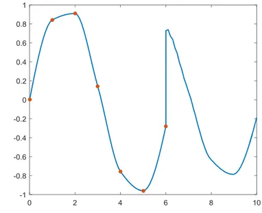
The figure 2.3 shows the interpolation in the previous case. PCHIP method features software to produce a monotone and "visually pleasing" interpolation to monotone data. Such an interpolation may be more reasonable than a cubic spline if the data contain both 'steep' and 'flat' sections.
5. PCHIP plus ARMA method
PCHIP is an excellent method to keep the shape of the curves when the data contain both 'steep' and 'flat' sections. But there is a deadly weakness: it cannot deal with the boundary interpolation. When there is some amount of lacking data on the boundary, it is not accurate to use PCHIP method to interpolate. In the meanwhile, it will bring the deadly disorder due to the property of the cubic interpolation.
For instance, if we want to interpolate until 10 in the example, the interpolation shows out as figure 2.4:
Figure 2.4: The example of boundary problem with PCHIP method
To overcome this issue, we used a PCHIP plus ARMA(autoregressive–moving-average) method.
In the statistical analysis of time series, ARMA models provide a parsimonious description of a (weakly) stationary stochastic process in terms of two polynomials, one for the autoregression and the second for the moving average.
Given a time series of data Xt , the ARMA model is a tool for understanding and,
perhaps, predicting future values in this series. The model consists of two parts: the autoregressive (AR) part and the moving average (MA) part. The (AR) part involves regressing the variable on its own lagged (i.e., past) values. The (MA) part involves modeling the error term as a linear combination of error terms occurring contemporaneously and at various times in the past.
The model is usually referred to as the ARMA(p,q) model where p is the order of the autoregressive part and q is the order of the moving average part.
1. Autoregressive model
The notation AR(p) refers to the autoregressive model of order p. The AR(p) model is written
1 p t i t i t i
X
c
X
(2-15)where
1,...,
p are parameters, c is a constant, and the random variable
t is white noise.Some constraints are necessary on the values of the parameters so that the model remains stationary. For example, processes in the AR(1) model with
1
1
are not stationary.2. Moving-average model
The notation MA(q) refers to the moving average model of order q:
1 q t i t i t i
X
X
(2-16)where the
1,...,
q are the parameters of the model, μ is the expectation ofX
t (often assumed to equal 0), and the
t,
t1,...
are again, white noise error terms.3. ARMA model
The notation ARMA(p, q) refers to the model with p autoregressive terms and q moving-average terms. This model contains the AR(p) and MA(q) models,
1 1 q p t t i t i i t i i i
X
X
X
(2-17)The general ARMA model was described in the 1951 by Peter Whittle, who used mathematical analysis (Laurent series and Fourier analysis) and statistical inference. ARMA models were popularized by a 1970 book by George E. P. Box and Jenkins[22], who expounded an iterative (Box–Jenkins) method for choosing and estimating them. This method was useful for low-order polynomials (of degree three or less).
Figure 2.5: The PCHIP plus ARMA interpolation method process
The figure 2.6 shows the result of the interpolation using PCHIP plus ARMA methd. Compared with the result of PCHIP method, the PCHIP plus ARMA methodis able to better capture features of the original data set.
\
Figure 2.6: The example of PCHIP plus ARMA interpolation in boader
2.2.4 Outliers processing
In statistics, an outlier is an observation point that is distant from other observations. An outlier may be due to variability in the measurement or it may indicate experimental
Input the data within the range [xmin,xmax]
PCHIP method to interpolate the missing data in [xmin,xmax]
ARMA method to predict the data out of the range [xmin,xmax] Start
error. The latter sometimes have to be excluded from the data set. An outlier can cause serious problems in statistical analysis.
In larger samplings of data, some data points will be further away from the sample mean than what is deemed reasonable. This can be due to incidental systematic error or flaws in the theory that generated an assumed family of probability distributions, or it may be that some observations are far from the center of the data. Outlier points can therefore indicate faulty data, erroneous procedures, or areas where a certain theory might not be valid. However, in large samples, a small number of outliers is to be expected.
There is no rigid mathematical definition of what constitutes an outlier, determining whether or not an observation is an outlier is ultimately a subjective exercise. There are various methods of outlier detection. Some are graphical such as normal probability plots, others are model-based or hybrid.
Considering that normally distributed data are common in the reality, here the outlier detection based on 3-σ rule is introduced.
In the case of normally distributed data, the 3-σ rule means that roughly 1 in 22 observations will differ by twice the standard deviation or more from the mean, and 1 in 370 will deviate by three times the standard deviation.[21] In a sample of 1000 observations, the presence of up to five observations deviating from the mean by more than three times the standard deviation is within the range of what can be expected, being less than twice the expected number and hence within 1 standard deviation of the expected number and not indicate an anomaly. If the sample size is only 100, however, just three such outliers are already reason for concern, being more than 11 times the expected number. The figure 2.7 shows the probability of the normally distributed data.
Figure 2.7: The possibility distribution for normal distributed data
Thus, as the equation shown below, 3-σ rule is used in the outlier detection in daily load. The daily load can be signed as
X
( ,
x x
1 2,...,
x
n)
with the mean valueX
and the standard deviation
, then we say thatx
i is an outlier ifx
i
X
3
orx
i
X
3
.2.3 Summary
In this chapter, the basic concept of load profile classifying and data processing is introduced. On one hand, the basic definition of load is introduced, together with five general load classifications: the load classification divided by physical performance, electrical energy, time scale, reliability and the international classification nowadays. On the other hand, the concept of load data preprocessing is introduced. According to the problems existing in the data preparing, the methods in the bad data processing, the data normalization, the missing value processing and the outliers processing are introduced. Especially in the interpolation of missing values, a method that combine PCHIP and ARMA interpolation is put forward to deal with the boundary problem.
3 BASIC CONCEPT OF PCA
3.1 Introduction of PCA
Principal component analysis (PCA) is an important statistical method to study how to convert multiple-index problems into fewer comprehensive indicators. Those few comprehensive indicators are not related to each other and can provide most of the information of the original indicators. PCA transforms high-dimensional space problems into lower dimensional one.
In addition to reducing the dimensions of multivariate data systems, PCA also simplifies the statistical characteristics of variable systems. PCA can provide many important system information, such as the location of the gravity center (or average level) of the data points, the maximum direction of data variation and the distribution range of the group points.
As one of the most important multivariate statistical methods, PCA has its applications in various fields such as social economy, enterprise management, and geology, biochemistry engineering. In comprehensive evaluation, process control and diagnosis, data compression, signal processing, model recognition and other directions, PCA method has been widely used.
3.2 Basic idea
The basic idea of PCA can be summarized as follows:
With an orthogonal transformation, the component-dependent original random variable is converted into a new uncorrelated variable. From an algebraic perspective, the covariance matrix of the original variable is converted into a diagonal matrix. From the geometric point of view, the original variable system is transformed into a new orthogonal system, so that it points to the orthogonal direction in which the sample points are dispersed, and then the dimensionality of the multidimensional variable system is reduced. In terms of feature extraction, PCA is equivalent to an extraction method based on the minimum mean square error.
3.2.1 Goal
The following considerations leads people to introduce PCA method when dealing with big data:[23]
(1) The number of components should be significantly less than the original number of data, preferably only one;
(2) The newly constructed components should reflect as much as possible the behavior and various information of the project under the original data;
(3) If there is more than one component, they should not be related to each other, and different components have different degrees of importance
3.2.2 Definition and property
Definition 1: Assume
X
(
X X
1,
2,...,
X
p)
is a p-dimensional random vector whose i th principal component can represent asY
i
u X i
i
,
1,2,...,
p
, Whereu
i is i th column vector of the orthogonal matrix U, and satisfies the following conditions:(1)
Y
i is the linear combination ofX X
1,
2,...,
X
p with the largest variance; (2)Y
k is irrelevant toY Y
1,
2,...,
Y
k1, where k=2,3,…,p.Property 1: Assume that
is the covariance matrix of the random vector1 2
(
,
,...,
p)
X
X X
X
, and its eigenvalues-eigenvectors pairs can be1 1 2 2
( , ),(
e
, ),...,(
e
p,
e
p)
, where
1
2
...
p
0
. So the i th component canbe: 1 1 2 2
...
,
1,2,...,
i i i i ip pY
e X
e X
e X
e X i
p
(3-1) Wherevar( )
Y
i
e
i
e
i
i,
i
1,2,...,
p
(3-2)cov( ,
Y Y
i k)
e
i
e
k0,
i
k
(3-3)Property 2: Assume that random vector
X
(
X X
1,
2,...,
X
p)
has a covariancematrix
, and its eigenvalues-eigenvectors pairs can be( , ),( , ),...,(
1e
1
2e
2
p,
e
p)
, where
1
2
...
p
0
. Yk is the main component, then:11 22 1 2 1 1
...
var(
)
...
var( )
p p pp i p i i iX
Y
(3-4)The property 2 shows that the covariance matrix
of the principal component vectors is the diagonal matrix
. The variance represents the variability and reflects the amount of information. It is easy to know from the above analysis that the total variance=11 22
...
pp
=
1
2...
p, that is the total amount of information can bemeasured by eigenvalues. The corresponding eigenvalues reflect the amount of information corresponding to the principal components. [24]
This leads to the following definition:
Definition 2: 1 k p i i
is the contribution rate for the k principal component,1 1 k i i p i i
isthe cumulative variance contribution rate of the first k principal components.
Property 3: If
Y
i
e X
i
is the principal component obtained from the covariance matrix
, then:( ,
k i)
ki k,
1, 2,...,
iie
Y X
i k
p
(3-5)is the correlation coefficient between component
Y
k and variableX
i , where1 1 2 2
Definition 3: The correlation coefficient index
( ,
Y X
k i)
between the k-th principal componentY
kand the i-th component of the original variableX
i is called the loading ofi
X
inY
k.However, it should be noted that
( ,
Y X
k i)
only measures the contribution of a single variableX
i to the principal component Y. When other Xj exists,
( ,
Y X
k i)
doesnot accurately indicate the importance of
X
j to Y. In practice, variables with larger (in absolute value terms) coefficients tend to have larger correlations, so importance measures for univariate and multivariate result to similar result. Therefore,
( ,
Y X
k i)
helps to explain the principal components.3.2.3 Basic algorithms and steps
The basic algorithms and steps of PCA can be shown below:
(1) Collect the sample workers of the p-dimensional random vector
1 2
(
,
,...,
p)
X
X X
X
, list observation data matrixX
(
x
ij n p)
;(2) Preprocess the raw data in the sample array converting the original data into positive indicators (the raw data preprocessing was already discussed in Chapter 2), and then use the following formula:
*
1, 2,...,
1, 2,...,
var(
)
ij j ij jx
x
x
i
n
j
p
x
(3-6)Where
x
j andvar(
x
j)
are the mean value and the standard variance of the j-th variables. Standardize the resulting data to obtain a standardized array Z.1 2 n
z
z
Z
z
(3-7)1
ij p pZ Z
R
r
n
(3-8)(4) Solve the Eigen-equation of sample correlation coefficient matrix R to obtain p eigenvalues
1
2
...
p
0
(5) Obtain the main component
Y
i
u X i
i
,
1,2,...,
p
, orY
UX
, where1 2 n
u
u
U
u
,
u
ij
z b
i
0j ,b
0j is the unit eigenvector.The corresponding PCA analysis process algorithm is shown in figure 3.1:
Figure 3.1: The corresponding PCA analysis process algorithm
3.3 Data process
In this section, PCA data processing is discussed.
3.3.1 Data requirements
A basic assumption of the PCA method is that the values of each case corresponding to each component obey the normal distribution.
Is PCA available in the problem?
raw data processing
raw data standarization
calculate correlation coefficient matrix R
Solve eigenvalues and eigenvectors of matric R
Solve the principle components Yes
Yes
other methods No
Usually, especially when the number of cases is large, the assumption is true. However, when the number of cases is small, or the degree of discretization of the criteria values is high, it cannot be assumed that the values of the component also follow the normal distribution. In addition, according to the Law of Large Numbers in mathematical statistics, as the number of evaluation objects increases, the average level and dispersion degree of evaluation indicators tend to be stable, so the covariance matrix also tends to be stable, increasing the accuracy of evaluation results. The PCA is suitable for comprehensive evaluation of large data set. Therefore, in this sense, the PCA method is not applicable to situations where the number of cases is small and the number of components is relatively large.
Similarly, when the PCA is used for multi-index calculation, the normalization (Z-Score) method is often used for dimensionless processing. The premise of standardized application is that the number of data is larger, and it is better to exceed the number of large samples and the sample data is much larger than the index.
On the other hand, the advantage of PCA is that it can turn related data into irrelevant data. In a sense, we also require that the original data have a certain degree of correlation. Otherwise, we lose the significance of applying PCA. In general, the relationship between indicator data is related to the following conditions:
(1) n variables are completely correlated
At this point, the n-1 variables are deleted, and the objects to be evaluated can be sorted. However, this is not really multivariate sorting, and PCA is not useful.
Since the principal components are mutually independent variables, that is, they meet the property 1; many literatures believe that the principal component analysis can eliminate multiple correlations of the original variables. However, in fact, the multiple correlations of variables will distort the real data information from both direction and quantity.
(2) n variables are completely uncorrelated
At this time, these variables cannot be compressed by PCA. Or, usually, the starting point variable correlation matrix of PCA becomes a diagonal matrix, and the de-correlation of PCA does not exist.
(3) There is a certain correlation between n variables
There are certain correlations between n variables, so you can use PCA to compress the data. In this case, the higher the degree of correlation between variables, the better the PCA works.
The relation between variable correlation and feasibility of PCA is shown in the figure 3.2. In real life, most of the indicator variables are not completely correlated, so the PCA is of great use.
Completely correlated variables Not completely correlated variables Completely uncorrelated variables Highly correlated Mid correlated Lowly correlated Calculate the Correlation matrix
PCA is not needed
PCA is not needed PCA has better
performance
PCA has less performance
Figure 3.2: The PCA application situations
Summarizing, when performing PCA, the following requirements are imposed on the data:
The number of data required should be large, so that the sample data is much larger than the index. It is not applicable to the case where the number of cases is small and the number of components is relatively large; the variables can have a certain correlation, but in practical applications, it is incorrect to artificially create multiple correlations for variables for comprehensive evaluation. Since most of cases can meet the above requirements in practical applications, therefore the application prospect of PCA is very broad.
3.3.2 Data standardization
The key to principal component analysis is to find the principal component, and its tool is the covariance matrix. Since the covariance matrix is susceptible to the dimension