Optimization with machine learning-based modeling: an application to humanitarian food aid

ALMA MATER STUDIORUM - UNIVERSIT `A DI BOLOGNA

DEPARTMENT OF ELECTRICAL, ELECTRONIC, AND INFORMATION ENGINEERING ”GUGLIELMO MARCONI”

SECOND CYCLE DEGREE IN

ENGINEERING MANAGEMENT

Master thesis

in

Optimisation Tools Laboratory

Optimization with machine

learning-based modeling:

an application to humanitarian food aid

Supervisor

Candidate

Prof. Valentina Cacchiani

Donato Maragno

Co-supervisor

Prof. Dick den Hertog

Graduation Session II

Academic year 2019/2020

Acknowledgements

S

Un grazie speciale a tutte le persone che mi hanno accompagnato lungo questo viag-gio. ´E a voi che dedico questo importante traguardo.

Contents

1 Introduction 3

2 Literature review 7

2.1 Operations Research-Machine Learning . . . 7

2.2 The humanitarian food aid . . . 8

3 The diet problem with palatability constraints 11 3.1 The diet problem: the origins . . . 11

3.2 Humanitarian Food Supply Chain model description . . . 11

3.3 The food basket palatability . . . 13

4 Data-driven optimization 15 4.1 Machine Learning model design . . . 17

4.1.1 Data collection . . . 17

4.1.2 Data preparation . . . 18

4.1.3 Model choice and training . . . 19

4.2 Embedding the Machine Learning model . . . 24

5 Case study: A palatable diet for Humanitarian Aids 26 5.1 Technical implementation . . . 26

5.2 Data collection for the case study . . . 26

5.2.1 On-site data collection using people’s opinions . . . 27

5.2.2 Artificial data collection using a food basket generator . . . . 28

5.3 Data preparation for the case study . . . 34

5.4.1 MLBO with Linear Regression . . . 35

5.4.2 MLBO with Artificial Neural Network . . . 35

5.5 Embedding the Machine Learning model for the case study . . . 36

5.6 Numerical results . . . 37

5.6.1 Specific Food Basket Generator . . . 44

6 Considerations 47

7 Conslusions and further research 50

Bibliography 53

1

Introduction

Operations Research (OR) is a discipline that has its origins in the Second World War, when it was used as a support for decision-making in the military field. The Association of European Operational Research Societies (EURO) describes OR as: “a scientific approach to the solution of problems in the management of complex systems. In a rapidly changing environment, an understanding is sought which will facilitate the choice and the implementation of more effective solutions which, typi-cally, may involve complex interactions among people, materials, and money” [2]. Nowadays, it is widely used in different types of industries, from finance to retail, from telecommunications to medical services, from oil and gas to industrial produc-tion. Regardless of the specific industrial application, Operations Research tools can support managers to make quantitative, better and more informed decisions. This is achieved through the implementation of mathematical models that represent the reality in which we operate and for which we look for a solution, possibly optimal. Model design and model resolution are two opposite activities, in the sense that, if on the one hand, the aim is to increase the accuracy in the representation of reality, on the other hand, it is necessary to consider the model complexity in terms of fea-sibility and time consumption. Models that poorly approximate the reality result in useless solution, too complex models make usually not possible to find an algorithm that runs in polynomial time in the size of the inputs and finds a global optimum. Generally speaking, a good model finds the right balance between model accuracy and model complexity.

In recent years, some research on the improvement of OR models, both in accuracy and complexity, has seen new forms of ”collaboration” with algorithms belonging to the field of Machine learning (ML). The term Machine Learning was coined by Arthur Samuel [37], an American IBMer and pioneer in the field of computer gaming

and Artificial Intelligence. Ron Kohavi refers to ML, saying that it is the application of induction algorithms as one step in the process of knowledge discovery[26]. These algorithms are used to build data-based mathematical models in order to make pre-dictions or decisions without explicit programming [27]. Like Operations Research, Machine Learning is widely used in various types of applications in any industry due to its unique flexibility.

The focus of this thesis is on the combination of Operations Research and Ma-chine Learning. The goal is to build a data-driven, rather than problem-driven, mathematical model through the integration of these two disciplines. Specifically, we will use an ML model to shape a constraint of an optimization model. This par-ticular type of integration is useful whenever we have to model one or more relations between the decisions and their impact on the system. These kinds of relations can be difficult to model manually, and so ML models are used to learn it through the use of data. This methods is very generic and can be applied whenever information can be inferred from data.

An example in which a data-driven approach has shown good results is presented in [29]. The authors work on two dispatching problems that consist of mapping a set of heterogeneous jobs on the platform cores so as to maximize an objective related to the core efficiencies. In this case, the Machine Learning model is used to predict the efficiency of each core according to various factors including temperature, workload, core position, and so forth.

Another example can be the use of Machine Learning models to predict the main-tenance of an industrial machine whose work schedule is defined by an optimization model. Knowing, dynamically, the probability of failure of a machine (or one of its components) it is possible to make more accurate scheduling that may involve more machines.

Our case study concerns the important issue of humanitarian food aid. We start illustrating an existing model that optimizes the flow of food throughout the hu-manitarian supply chain, minimizing the total costs in order to feed more people in

need. Then, we focus on the diet sub-problem implementing an ML-based model that takes into account the ration palatability. Since the palatability constraint (es-pecially when we have to consider people’s opinions rather than just general rules) is difficult to express in a mathematical way, we use Machine Learning to learn it au-tomatically. The process to derive an optimization model which includes a Machine Learning-based component is divided into four steps:

• Data collection. Data collection is necessary to get an idea of the opti-mization model structure and to train the ML models that will be used as a constraint. The data collection process may involve the external environment, or, like in our case study, can be the result of an artificial data generator.

• Data processing. Data processing involves a series of tasks to improve the quality of the dataset and make it suitable for model training. This phase includes data cleaning and data transformation activities.

• Building and training of the ML model. Once the dataset is structured and the data is pre-processed, the ML model has to be designed and trained taking into account the trade-off between model complexity and accuracy.

• Embedding the ML model into the optimization model. Once the ML model has been trained, it can be embedded into the optimization model to build a data-driven constraint or (part of the) objective function.

The remainder of the research is structured as follows. In Section 2.1, the relevant literature regarding the integration of Machine Learning and Operations Research is reviewed. The literature review on humanitarian supply chain management, which is the baseline scenario in the case study, follows in Section 2.2. In Section 3, the importance of the optimal diet and its palatability are discussed. In Section 4, the new data-driven approach is explained in detail. A real application of this approach is described in Section 5 with a case study that includes all the steps mentioned in the previous section. In Section 5, are also discussed the results obtained from the case study. Then, in Section 6, the data-driven approach is analyzed with the

pros and cons that emerged during the case study. Lastly, conclusions and possible subjects of further research are outlined in the final Section 7.

2

Literature review

2.1

Operations Research-Machine Learning

In this research, we focus on a particular approach where ML is used to improve an OR model, however, it should be noted that the OR-ML combination is not one-way. Well-known and extensively studied OR algorithms can improve or even replace ML models in some cases. A perfect example comes from the field of Explainable Arti-ficial Intelligence XAI, where exact approaches such as Optimal Classification Tree [6] or Boolean Decision Rules via Column Generation [12] report results compa-rable to state-of-the-art ML models in terms of accuracy, but with a much higher degree of explainability. Another example is presented by Fischetti and Jo where a Mixed-integer Linear Programming (MILP) model is used for feature visualization and the construction of adversarial examples for Deep Neural Networks (DNNs) [16].

Focusing on how Machine Learning can support Operations Research, the survey titled ”Machine Learning for combinatorial optimization: a methodological tour d’horizon” [5] reports various situations in which ML models can improve the reso-lution of OR problems. The authors point out that from an optimization perspective, Machine Learning can help improve optimization algorithms in two ways:

• Replace some heavy calculations with fast approximations. In this case, learn-ing can be used to construct these approximations in a general way without the need to derive new explicit algorithms.

• Expert knowledge is not complete, and some algorithm decisions can be del-egated to the learning machine to explore the decision space and hopefully implement good decisions.

For example, some research has been conducted on new approaches for branch and bound (B&B) algorithms. One of these approaches considers a special type of

deci-sion tree that approximates strong branching decideci-sions and decides on what variable to branch next [30]. For a complete survey on this type of B&B algorithms we refer to [28].

Another way to combine ML and OR is to use the first one to build (part of) the optimization model replacing, or supporting, the (traditional) manual model building. According to [29], this approach is able to (i) use data in order to learn relations between decision variables (decidables), and their impacts (observables), and (ii) encapsulate these relations into components of an optimization model, i.e., objective function or constraints.

The idea of using ML to learn and define parts of the optimization model that are difficult to derive manually is the central theme of this thesis. According to [13], this approach allows for using data to define specific models for specific problems, does not require domain experts to the same extent as traditional modeling, can be less expensive in terms of money and time, and is easily adjustable to changes in the scenario.

It paves the way for a powerful type of optimization model building but brings with it a series of new tasks to perform and some drawbacks to consider. Therefore, it is essential to have a clear idea of the scenario in order to evaluate the need for transparency, the accessibility of data, and the trade-off between complexity and accuracy.

2.2

The humanitarian food aid

The case study of this research focuses on one of the key points in the humanitarian aids research area: the distribution of food in geographical areas that have been/are subject to natural (e.g. hurricanes, earthquakes, floods) or human-made (e.g. wars, oil spills) disasters. According to the Food and Agriculture Organization (FAO) report (2020) [15], in today’s world, there are more than 689 million undernourished people in the world, accounting for 8.9 percent of the global population. It is esti-mated that by 2030 (the year the United Nations has set the goal of achieving the

zero hunger challenge of sustainable development [43]), this number will increase to more than 840 million. According to the new studies conducted by the World Food Programme (WFP) [45], due to the COVID-19, the number of people facing starvation is expected to skyrocket if no new plans are implemented. The WFP is the world’s largest humanitarian organization addressing hunger and promoting food security. It provides food assistance to an average of 91.4 million people in 83 countries each year, with more than 16,000 employees across the globe [44].

In a more general setting, providing aid to vulnerable people is the core purpose of the humanitarian supply chain management (HSCM) [41]. HSCM aims to ensure the prioritization of needs, and hence to respond to affected people by using given re-sources efficiently during and after a disaster [46]. Within HSCM, Altay and Green split the disaster management into 4 stages: mitigation, preparedness, response, and recovery [1]. The first two stages occur before the disaster (pre-disaster) and involve all necessary preventive measures to avoid/minimize the negative impacts. The third and fourth stages involve short-term response after the disaster (post-disaster) and long-term reconstruction to restore the affected communities to their pre-disaster condition [38]. The post-disaster relief and reconstruction phase is one of the most difficult tasks, both in terms of planning and coordinating. It includes or-der fulfillment, demand and supply management, human resource management, and performance evaluation [24]. Nevertheless, according to [8], most of the literature on humanitarian logistics focuses on disaster preparedness and response, making long-term recovery a neglected topic. Only a few mathematical models cover the entire scope of the humanitarian supply chain. In these cases, attention is focused on (a combination of) three sub-problems, namely facility location [3], distribution [19, 31, 36] and, inventory control [4, 34].

Because of this gap in mathematical formulations for post-disaster relief, Peters et al. [32] developed a deterministic linear model (Nutritious Supply Chain (NSC) model from now on) which integrates multiple supply chain decisions such as food basket design, transfer modality selection, sourcing, and delivery plan. The various

successful applications of the NSC model fostered us to use its basic version (with no cash and no voucher modalities allowed) as the starting point of our research.

3

The diet problem with

palata-bility constraints

In this section, first, we present the origin of the diet problem, and then describe how it is considered in the NSC model. Finally, we describe the palatability constraint and what makes it so interesting.

3.1

The diet problem: the origins

Back in 1945, George Stigler, winner of the 1982 Nobel Prize in Economics, pub-lished the paper ”The Cost of Living” [39]. Stigler proposed the following problem: ”For a moderately active man weighing 154 pounds, how much of each of 77 foods should be eaten every day so that the man’s intake of nine nutrients will be at least equal to the Recommended Dietary Allowances (RDAs) suggested by the National Research Council in 1943, with the cost of the diet being minimal?” The problem, initially solved by a heuristic method, became, according to G. Dantzig [11], the first large-scale problem solved by using the Simplex Method by Jack Laderman in 1947.

Since 1945, many variants of the diet problem have been developed [14, 33, 17], each of them tailored to a specific situation. In Peters et al. HSCM, dietary issues represent a relevant part of the model. A brief description of the NSC model is required before delving into the diet formulation.

3.2

Humanitarian Food Supply Chain model

de-scription

The model formulated by Peters et al. [32] is a combination of a capacitated, multi-commodity, multi-period network flow model and a diet problem via the addition

of nutritional components and requirements. In the humanitarian supply chain, the suppliers are modeled as source nodes, the discharge ports and WFP warehouses are considered transshipment nodes, and the demand nodes are the Final Delivery Points (FDPs), where the demand is dependent on the food basket and the number of beneficiaries.

Suppliers are divided into international, regional, and local suppliers. International suppliers refer to suppliers located outside the mission country, regional suppliers refer to suppliers within the mission country, and local suppliers indicate the FDPs markets. Supply nodes are the only places in the network were goods can be procured and enter the network. After the goods enter the network, they are transported to transshipment nodes, locations in which food can be temporarily stored before being shipped to Final Delivery Points. The FDPs are the locations of beneficiaries, these are modeled as the endpoint of the humanitarian supply chain.

The objective function is composed of transportation costs, storage costs, handling costs in suppliers’ nodes, and other costs such as milling, packaging, monitoring, reporting, etc. Constraints affect the flow of commodities, purchasing, transporta-tion and processing capacity, the degree of satisfactransporta-tion of nutritransporta-tional needs, and the amount of each commodity. The demand is defined as nutritional requirements. This allows to optimize the food baskets, rather than using pre-defined ones. In this way, it is necessary to provide accurate information about the nutritional value of different foods, as well as the minimum nutritional requirements for the average person. In this thesis, we used the daily nutrient requirements presented in the re-port ”Planning a Ration” by the World Health Organization (WHO) [42]. Further adjustments can be done depending on the demographics, ages, city/country tem-perature, and other factors. For example, according to WHO (Table 3.1), with an average temperature of 20 degrees Celsius or higher, the daily energy requirement is 2100 kcal. A reduction of 5 degrees means that daily energy intake will increase by 100 kcal, a further decrease of 5 degrees will require another 100 kcal, and so on.

Adjustments to energy requirement mean daily temperature 20◦C 15◦C +100 kcal 10◦C +200 kcal 5◦C +300 kcal 0◦C +400 kcal

Table 3.1: Source: The management of nutrition in major emergencies. WHO. Geneva, 2000.

In this study, we consider only average values and these values are reported in Table A.1 and A.2 shown in the Appendix.

3.3

The food basket palatability

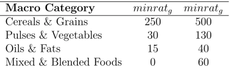
According to [32], their NSC model aims to generate food baskets that address the nutrient gap, are distributable, and palatable. The definition of palatability is based on constraints that limit the maximum and minimum quantity of each food in the basket. These constraints are used to avoid solutions with extreme (too high or too small) values. For example, solutions with more than half a kilogram of peas or 200 grams of oil in a daily ration would be considered unpalatable. Therefore, in the NSC model, there are five constraints, one for each macro category of foods, that impose upper and lower bounds to the amount of food per category. These limits are based on ”unwritten rules” quantified with the help of nutrition experts and food basket designers.

Macro Category minratg minratg

Cereals & Grains 250 500 Pulses & Vegetables 30 130

Oils & Fats 15 40

Mixed & Blended Foods 0 60

Table 3.2: These ration sizes are tailored for General Food Distribution (GFD), which is the bulk of WFP distribution. Source: Peters et al. (2016)[32]

This approach can, with a high degree of approximation, include some socio-cultural aspects in the constraint’s formulation (e.g. an higher limit of rice for Asians) but it is very unlikely that it also considers subjective components. This

may drive to food baskets whose palatability score is misleading and far from the beneficiary’s opinion. Moreover, this approach forces the ration to be palatable but does not provide the flexibility to impose varying degrees of palatability.

Considering that much of the information useful for modeling this constraint can be derived from beneficiaries’ opinions, we decided to use, in our research, a Machine Learning model for extracting information and using it to model the palatability constraint. In this scenario, a data-driven constraint has the potential to model (implicit) cultural, social, and geographic factors in a very insightful way. Moreover, this constraint can be used with different palatability scores to ensure a higher degree of flexibility.

4

Data-driven optimization

The general process to describe a scenario with a mathematical programming formu-lation, and solve it, is composed of problem identification, mathematical modeling, solution analysis, decision-making, and evaluation of the results obtained through the use of simulators or real applications. Usually, the most complex part is the mathematical modeling, where a full understanding of optimization tools and the scenario to be modeled is essential. From the point of view of accuracy, a good optimization model must be both inclusive (i.e., it includes what belongs to the problem) and exclusive (i.e., shaved-off what does not belong to the problem). An inaccurate model can lead to optimal, but useless solutions. A very accurate model could be extremely complex to solve.

The worst situation would be if a complex formulation is also inaccurate. This is more likely if the relations between decisions and system observations are man-ually translated into mathematical formulations.

The purpose of this research is to show how Machine Learning algorithms can be used to learn the relation between decidables and observables, on the system. One of the main reasons why these algorithms can be used is to replace, or complete, the traditional problem-driven constraints, relieving the OR expert from the onerous task of manual modeling, whenever the translation into mathematical constraints turns out to be extremely complex or is not possible because of lack of knowledge. Among the different positive aspects, this approach has consequences in terms of accuracy and the ability to adapt to changes in the scenario. We will see it in the case study and in the final considerations.

The Machine Learning-based Optimization (MLBO) model typically has the following structure:

min x,z f (x, z) (4.1) s.t. (4.2) gj(x, z) ≤ bj ∀j ∈ J (4.3) z = h(x) (4.4) x ∈ D (4.5)

where, x represents the decidables in domain D, and z is the vector of observables, which is inferred from the target system, and that we are modelling with the use of h(x). The h(x) vector of functions is the encoding of the ML model that describes those parts of the system where the relationship between observables and decidables is highly complex to model manually. Both the objective function f(x,z) and the constraint functions gj(x, z) can be based on a combination of decision variables and

observables.

In order to design a model with the structure just presented, there are three steps to follow:

1. Optimization model formulation. In this phase OR experts, in collabo-ration with domain experts, formulate a general structure of the optimization model. They decide what should be the objective function, what are the decision variables, and what is the design of those constraints that can be effi-ciently (right trade-off between accuracy and complexity) built in a traditional problem-driven way.

2. Machine Learning model design. This phase includes data collection, data processing, the choice of the Machine Learning algorithm to embed, its training, and evaluation. This step is not trivial, and it may take a long time to make the model accurate.

3. Embedding the trained Machine Learning model into the optimiza-tion model. It is possible to embed an ML model into an optimizaoptimiza-tion model

only if the former one is encoded so that it can be exploited by the optimization solver for the search process.

Since the first step is to define the optimization model and the process depends on the application, we will present it directly in the case study (Chapter 5). A complete explanation of the second and third steps is provided in the following sections.

4.1

Machine Learning model design

In this paragraph, we present the process of developing a Machine Learning model. Usually, it consists of: data collection, data preparation, model choice, and model training. In order to perform these steps in the best way, it is necessary that the general structure of the optimization model is already defined. With clear informa-tion about the decision variables and the observables, it is easier to identify what are the inputs and what should be the output of the ML model. Questions such as: “What are we trying to predict?”, “What are the target features?”, “How is the target feature going to be measured?”, “What kind of problem are we facing?” can help to identify the necessary tasks to perform.

Now, we discuss those steps that require special attention in the MLBO context.

4.1.1

Data collection

The process of gathering data is an essential step to maintain the correctness of the model since the quality and quantity of data has a direct influence on the final model performance.

The dataset for the learning techniques can be harvested from the real system or extracted from a simulator based on the real system. In the former case, we use methods such as observations, surveys, or interviews. Often these methods are very expensive in terms of time (for example, data gathering may involve manual activi-ties that are much slower than automated processes) and money (for example, the use of ad hoc sensors), but no, or few, assumptions and approximations are needed. An alternative is to use software that simulates reality in order to collect data. This method may be faster than previous methods, usually cheaper, and very flexible.

However, it can lead to poor approximations of reality, and therefore to a useless dataset. Hence, it must be performed in an accurate way.

Whenever we deal with MLBO, the trained Machine Learning model is applied to all those solutions that the solver evaluates during the optimization process. On these solutions, the ML model can perform very badly if the dataset is composed especially by the most likely solutions that can occur in the scenario. To avoid this problem, we have to realize a dataset that covers the entire space of solutions as uniformly (and unbiased) as possible [29].

4.1.2

Data preparation

Once we have the dataset, it can be necessary to clean and transform raw data into a form that can readily be used to train the Machine Learning model. Cleaning refers to the operation such as deleting irrelevant data and outliers or filling in missing values. Transforming data is the process of updating the format or value entries to reach a well-defined outcome. In the latter process are included tasks such as labels and features extraction, feature scaling, and data splitting into training, validation, and test sets:

• Training dataset. It is used to fit the model.

• Validation dataset. It is used to provide an unbiased evaluation of a model fit on the training dataset while tuning model parameters, also known as hyper-parameters.

• Test dataset. It is used to provide an unbiased evaluation of a final model fit on the training dataset.

Labels and features extraction is a critical process that impacts the final performance of the ML model. In the MLBO, we can decide to feed the Machine Learning model with (part of) the decision variables, or/and with their mathematical combinations. To use more complex features they must be encoded in the MLBO model by using specific constraints for feature extraction. If on the one hand, it can improve the

accuracy of the ML model, on the other hand, it can also increase the computational complexity of the final model optimization.

4.1.3

Model choice and training

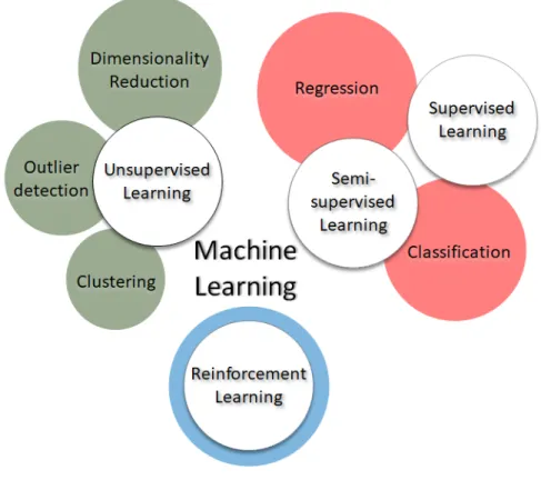
A good knowledge of the main Machine Learning algorithms is necessary to identify the algorithms that would perform best in the application of interest. Generally, Machine Learning algorithms are divided in four types of Learning: supervised, unsupervised, semi-supervised and reinforcement (Figure 4.1):

• In Supervised Learning, the dataset is a collection of labeled examples {(xs, ys)}Ns=1 where xs is a vector of features, in our case represented by the

decidables, and N is the number of samples s in the dataset. Each of the features contains information about the system that we are studying. ysis the

label associated with xs and it can be either an element belonging to a finite

set of classes (also called categories), or a real number, or a more complex structure, like a vector, a matrix, a tree, or a graph. These algorithms are used for regression and classification problems to predict the label associated with a vector of features passed as input to the trained model.

• In Unsupervised Learning, the dataset used to train the model is a col-lection of unlabeled examples {xs}Ns=1. In this case, the goal is to create a

model that takes as input a vector of x and searches for patterns and informa-tion that was previously undetected. These algorithms are used in clustering, dimensionality reduction, and outlier detection.

• In Semi-supervised Learning, a dataset combines a small amount of labeled data with a large amount of unlabeled data. The goal is the same as that of supervised learning, but it is hoped that using many unlabeled examples can help the learning algorithm to compute a better model.

• In Reinforcement learning, the algorithm interacts with an environment and is capable of perceiving the “state” of that environment as a vector of features. The algorithm is able to perform actions based on the current state, and it gets rewards based on the goodness of taken actions. The goal of this

kind of algorithm is to learn a function, also known as policy, that takes as input the state vector and outputs the optimal action to take.

We refer to [40, 18] for a more comprehensive explanation of these algorithms.

Figure 4.1: Types of Learning

Once we have identified the type of algorithms suitable for our problem, it is time to choose the specific algorithm that, once trained, will return better results on the test set. The processes of model training and quality assessment are widely studied in the literature [35, 21]. In a traditional application, the accuracy is measured with metrics such as Means Squared Error (MSE) or the number of correctly classified instances. However, in MLBO, the quality assessment can be compromised since the ML model has to work with instances that correspond to the solutions evaluated by the optimization solver. Often, these instances, favored in terms of objective function cost, are not present, or are but in a relatively small number, in the test set. If the machine learning model performs poorly in these situations, the quality assessment performed on the test set will not highlight this issue and will result in optimistic accuracy values. We will deepen it in the case study, where a solution to

this problem is presented.

In traditional Machine Learning applications, evaluating the model is usually a mat-ter of accuracy, and the computational complexity is often overlooked. In MLBO, when we talk about ML-model complexity, we refer to the size and linearity of the trained model. This architectural complexity has an impact on the MLBO model resolution both in terms of time to solve and in terms of optimality guarantees. This leads to a trade-off between accuracy and complexity in the choice of the predictive model. Two Machine Learning models antipodal in terms of architectural com-plexity are Linear Regression (linear model) and Artificial Neural Networks (highly nonlinear model).

Linear Regression

(Multiple) Linear regression (LR) is a supervised algorithm for regression problems. A Linear Regression model takes as input a vector x ∈ Rn_{of decidables and predicts}

the value of a scalar Y ∈ R that is called dependent variable. The output is a linear function of inputs and the general formula is:

Y = xβ + ε, (4.6)

where β ∈ Rn is the vector of parameters, or weights, and ε ∈ R is the intercept. Different techniques can be used to train the linear regression model from data, the most common of which is called Ordinary Least Squares (OLS).

In the basic case, with no regularization terms, the architectural complexity of Lin-ear Regression models is usually low due to the model linLin-earity and the number of parameters that is equal to the number of variables plus the intercept. If, on the one hand, the simplicity of the model makes it very attractive for embedding in OR models, on the other hand, if the relation between x and Y is nonlinear we have poor performances that make the model useless in practice.

performance of LR used as a constraint of an MLBO model.

Artificial Neural Networks

Artificial Neural Networks (ANNs) are biologically inspired models whose basic unit is called node, or neuron. According to Haykin [22], a neuron k can be described mathematically by the following equations:

vk = n X i=1 wkixi (4.7) yk= ϕ(vk+ bk), (4.8)

where vk is a linear combination of inputs x1, x2, ..., xnand weights wk1, wk2, ..., wkn.

The bias bk aims to increase/decrease the net input of the activation function. ϕ(·)

is the so-called activation function, which is a nonlinear, monotonic, non-decreasing function. yk is the output of neuron k (Figure 4.2).

Figure 4.2: Scheme of an artificial neuron. Source: Haykin (2009)[23]

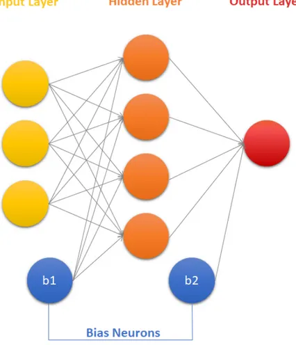
Typically, neurons are aggregated into layers and the number of layers defines the depth of the ANN. The first layer is the input layer, the last one is the output layer, and those in the middle are called hidden layers. Each neuron has inputs and produces a single output which can be sent to multiple other neurons. The

input can be derived from the feature values of external data, or it can be derived by the output of the neurons in the previous layer. The outputs of the final layer accomplish the predictive task.

The ANN architecture used for the case study is a Fully Connected Neural Net-work (FCNN) where all the neurons in one layer are connected to the neurons in the next layer (Figure 4.3).

Figure 4.3: Fully Connected Neural Network architecture

Generally, ANNs are very flexible and adaptable to different scenarios, resulting in good performance even with little domain knowledge. However, the disadvan-tage is that Artificial Neural Networks have a complex architecture. In FCNN, the number of trainable parameters is much higher than the number of features per sample. They depend on the input size, the number of nodes and the number

of deviations.

If an FCNN is composed of one hidden layer with h nodes, an input layer with i nodes, and an output layer with o nodes:

number of parameters = (i × h + h × o)

| {z }

connections between layers

+ (h + o) | {z }

biases in every layer

In addition to a large number of parameters, another thing that makes ANNs com-plex models is their nonlinearity. Activation functions such as the hyperbolic tan-gent, or the sigmoid make the model nonlinear, and consequently also the MLBO model. It has a huge impact in terms of computational complexity both to train the predictive model and (mainly) to optimize the final MLBO model.

4.2

Embedding the Machine Learning model

Embedding an ML model into an optimization model is the last step. A successful embedding would allow us to take full advantage of the optimization solver’s poten-tial. According to [29], the ability to embed ML models into optimization models plays a key role in bridging the gap between predictive and prescriptive analytics. The embedding process requires that the Machine Learning model trained in the previous step is mathematically “explainable” in the form of decision variables and trained parameters.

The integration of an LR model, thanks to its linear structure, has no significant impact on the complexity of the final optimization model. Furthermore, if the final model belongs to the class of Linear Programming (LP), algorithms such as the Interior-points Method would guarantee an optimal solution in polynomial time. The optimality guarantees, however, do not give information in terms of accuracy of the ML component. If the regression model performs poorly in the MLBO model, the final solution, still optimal for the MLBO model, will be useless and not appli-cable to the studied system.

it is possible to integrate each node of the neural network individually through the use of decision variables, parameters, and their own activation function. Afterwards, it is possible to combine them in order to obtain a single function that outputs the prediction of the neural network. The same process can be done in a single step, embedding the entire ANN starting from the output layer to the input layer. There-fore, if on the one hand, a large number of nodes and layers allows a more accurate description of nonlinear functions, on the other hand, the embedding of these models becomes more complicated to perform.

Unlike LR, with ANNs the final problem is a Mixed Integer Nonlinear Programming (MINLP). As long as the activation functions are supported by the MINLP solver, the integration process is feasible. With nonlinear activation functions, the MINLP solver will converge to a local optimum, possibly different from the global optimum, but still useful for the studied problem.

5

Case study: A palatable diet for

Humanitarian Aids

In this chapter, we explore how Machine Learning is used to mathematically model the ration palatability in a diet problem formulation within the HSCM scenario. We will describe how data is collected, how it is processed, and which ML models are used. Then we will proceed with the description of the MLBO model and the results obtained. Finally, we will highlight some critical issues of the MLBO model and what are the possible causes and remedies.

5.1

Technical implementation

The optimization modeling language used for the case study is Pyomo. Pyomo is an open-source software package that supports a diverse set of optimization capa-bilities for formulating, solving, and analyzing optimization models [20]. All the optimization models are taken over by NEOS server, which is a free internet-based service that provides access to more than 60 state-of-the-art solvers [10]. We adopted CPLEX v12.9 [9] to solve LP models, and KNITRO v12.2 [7] to solve MINLP mod-els.

We executed the calculations on a standard Windows 10 laptop machine featuring an Intel i7 8565U and 8 Gb RAM.

5.2

Data collection for the case study

To build a palatability constraint based on Machine Learning, it is necessary to define the dataset that will be used to train and assess the ML model. Data collection is a process whose difficulty depends very much on the type of application being considered. In our case, each sample contains a set of features represented by the quantity of each food and a label represented by the palatability score associated with that food basket. In order to collect the palatability scores, beneficiaries must

provide feedback on the goodness of different rations. As this is a difficult task to be performed in practice, especially within a short time period, we decided to build a generator of food baskets, and a set of rules to evaluate each basket in terms of palatability. In both cases, a well-defined scale must be used to classify food baskets from the most palatable to the least palatable.

5.2.1

On-site data collection using people’s opinions

The first way to collect data is to generate food baskets with different quantities and combinations of foods and then place them under the judgment of beneficiaries. One could also ask them directly to design rations that have different palatability values. This approach has the great advantage of reaching people’s subjective opinions, which implicitly contain all the factors related to social and cultural influences. However, there are some drawbacks to consider:

• Coordination complexity. Involving people, especially in complex situations such as those where WFP operates, requires good collaboration between bene-ficiaries and humanitarian organizations. Data collection can be done through interviews or questionnaires that may require standardized forms, a central-ized database, and the use of heterogeneous tools (digital and/or traditional). Bad coordination would increase the impact of the following points.

• High costs. Collecting data requires expensive tools for data acquisition, stor-age, and maintenance. In addition, it requires specialized personnel to handle data-related operations.

• Limited number of iterations. The data collection process can be performed in several and separate stages depending on the type of data we need. As we will describe in section 5.6.1, to improve the MLBO model we proceed with an iterative data collection process. This may not be possible, for economic and limited time reasons, when we deal with on-site data gathering.

Despite the drawbacks, we believe that with sufficient resources and a good orga-nization of activities, it is possible to carry out field data collections increasing the

scenario representativeness in the dataset. In our research, it was not possible to use field data as it is not yet available and laborious to gather in a short time.

5.2.2

Artificial data collection using a food basket generator

To generate a large number of different food baskets, we developed the Food Basket Generator (FBG) which is a mathematical optimization model with parameters (highlighted in teal) that allow getting different solutions at each run. We underline that FBG is not the optimization model that provides the best palatable food basket, but is only used for generating data on food basket palatable scores, in place of collecting data directly from the beneficiaries. The palatability score corresponding to each food basket is based on a function we defined and described just after the model presentation.

We want to specify that from now on, we will talk about daily food baskets. Deciding whether to change these baskets daily, weekly, or monthly is beyond the scope of this article. However, we expect that the resulting baskets will remain the same for a period of time that guarantees efficient quantities of food also under other cost items (e.g., purchase, transport, storage). This means that if in a daily food basket we have 20 grams of meat, and the food basket remains unchanged for 30 days, we must consider 600 grams of meat per person. The same is true for all the other foods that make up the basket, assuming that the ration palatability remains unchanged and that it does not depend on the size of the time period.

Food Basket Generator model

We use the same notation as in Peters et al.[32], adapted to our situation.

Set Description

K Set of commodities (k ∈ K)

G Set of food macro categories (g ∈ G) L Set of nutrients (l ∈ L)

Gabsence

Set of commodities that must be kept below a certain threshold (Gabsence ⊂ K)

Gpresence

Set of commodities that must be kept above a certain threshold (Gpresence ⊂ K)

Parameter Description

N utreql Nutritional requirement for nutrient l ∈ L (grams/person/day)

N utvalkl Nutritional value for nutrient l per gram of commodity k ∈ K

minratg

Lower limit per commodities macro category g ∈ G (grams/person/day)

maxratg

Upper limit per commodities macro category g ∈ G (grams/person/day)

randomT hresholdp

Threshold used as lower

bound to the amount of those foods k ∈ Gpresence

randomT hresholda

Threshold used to upper

bound to the amount of those foods k ∈ Gabsence

palat rangeg

Random value in the range [0,maxratg−minratg

2 ]

∀g ∈ G (grams/person/day)

Table 5.2: Parameter notation used in the FBG model

Parameter Description

Sl Realized shortfall of nutrient l in percentage

xk Amount of commodity k measured in hectograms

P alatabilityComponentg

Distance between the amount of food in category g and the point maxratg+minratg

2 ∀g ∈ G

Table 5.3: Variable notation used in the FBG model

Objective function

The objective function in the traditional model for the diet problem is a minimization of costs. In our case, we minimize nutrient shortfalls (5.1). This choice is based on the model structure where Slvariables can result in values that make the food basket

feasible but not meaningful if they do not constrained or used as part of the objective function. The loss in practical meaning happens because most of the nutrients do not reach the minimum requirements. We decided to avoid constraints on Sl and

use them in the objective function (assuming that all the nutrients have the same importance) to expand the space of feasible solutions. Nevertheless, if we want to minimize the cost, it is completely possible, but we have to impose upper bounds on Sl variables. min x,S X l∈L Sl (5.1)

Constraints

X

k∈k

N utvalklxk≥ N utreql(1 − Sl) ∀l = 1... |L| (5.2)

Constraints (5.2) ensure the nutrient requirements, although allowing for the use of shortfalls. Sl variables constrained to be in the range 0-1 (5.10).

minratg ≤

X

k∈g

xk ≤ maxratg ∀g ∈ G (5.3)

Constraints (5.3) bound the amount of food for all the five macro categories in order to consider only solutions with a minimum value of palatability according to Peters et al. [32].

xk ≥randomT hresholdp ∀k ∈ Gpresence (5.4)

xk ≤randomT hresholda ∀k ∈ Gabsence (5.5)

xsalt ≥ 0.15 (5.6)

xsugar ≥ 0.5 (5.7)

Constraints (5.4) and (5.5) are used respectively to force the presence of a certain type of commodity in the final solution and to exclude other commodities from it. For a feasible formulation we must have Gpresence∩ Gabsence = ∅. Constraints (5.6)

and (5.7) are used to bound the only two commodities, salt and sugar, that do not belong to any category.

X

k∈g

100xk− P alatabilityComponentg =

maxratg+ minratg

2 ∀g ∈ G (5.8)

−P alat rangeg ≤ P alatabilityComponentg ≤P alat rangeg ∀g ∈ G (5.9)

With constraint (5.9), we give to the optimization solver the flexibility to choose P alatabilityComponentg within a randomly generated range of feasible values.

P alatabilityComponentg will be chosen so as to minimize the objective function as

category g thanks to constraints (5.8).

0 ≤ Sl ≤ 1 ∀l ∈ L (5.10)

xk≥ 0 ∀k ∈ K (5.11)

Constraints (5.11) are used to impose the amount of each commodity to be greater than or equal to 0.

How to ensure a different solution at each run

The FBG is a LP model where some of the components are randomly set during the model setup. The constraints (5.8), (5.9), (5.4), and (5.5) are used to define a different search space at each run. This means that, when the optimization solver searches for the globally optimal solution, has to explore a different space of solutions every time the optimization process is launched.

CPLEX is the solver used to find the optimal solution at each run. It is possible to generate more than one hundred of different solutions in one minute with a computation time per execution of about 0.06 seconds.

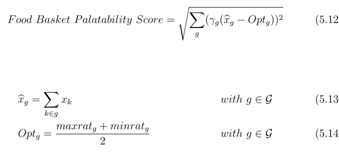
Food Basket Palatability Score

Once performed the optimization process, we have a solution with five

P alatabilityComponentg values, one for each macro category. To combine these five

values in a single palatability score (the desired label), we defined a formula based on the following idea: the closer the P alatabilityComponentg variables are to

zero, the higher the basket palatability score. This formula assigns to assign different scores depending on the amount of food. In other words, we call optimal point the center of each macro category range shown in Table 3.2, and we assign higher palatability scores to those solutions that have the sum of food per macro category closer to the optimal point.

More precisely, we aim to penalize the more those solutions that are the closer to the boundaries minratg and maxratg, hence, we use the Euclidean Distance Function

to define the score:

F ood Basket P alatability Score = s X g (γg(bxg− Optg)) 2 _(5.12) where b xg = X k∈g xk with g ∈ G (5.13) Optg = maxratg+ minratg 2 with g ∈ G (5.14)

Since the macro categories g have different range sizes, we use γg to balance the

impact of each of them on the score. The function used to calculate γg is (5.15) and

the values are displayed in table 5.4.

γg =

max{g∈G}(maxratg− minratg)

maxratg− minratg

(5.15)

Macro category γg

Cereals & Grains 1 Pulses & Vegetables 2.5

Oils & Fats 10

Mixed & Blended Foods 4.16 Meat & Fish & Dairy 6.25

Table 5.4: γg values for the five macro categories.

With (5.12), we get a palatability score that goes from 0 to 279.96 where 0 represents the highest palatability and 279.96 the worst one.

In order to get higher scores associated with higher palatabilities we reversed the score by this expression:

F ood Basket P alatability Score = 279.96 − F ood Basket P alatability Score

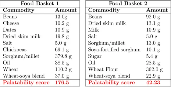
In Table 5.2 we see two examples of daily food baskets generated through the FBG and their palatability score.

Food Basket 1 Food Basket 2

Commodity Amount Commodity Amount

Beans 13.0g Beans 92.0 g

Cheese 10.2 g Dried skim milk 13.1 g

Dates 10.9 g Milk 10.9 g

Dried skim milk 19.8 g Salt 5.0 g

Salt 5.0 g Sorghum/millet 13.0 g

Chickpeas 69.1 g Soya-fortified sorghum 10.1 g

Sorghum/millet 379.8 g Sugar 5.4 g

Oil 38.5 g Oil 28.5 g

Wheat 110.2 g Wheat Flour 362.0 g

Wheat-soya blend 37.0 g Wheat-soya blend 22.9 g Palatability score 176.5 Palatability score 42.23 Table 5.5: Two examples of daily food baskets generated by the FBG.

Figure 5.1 is a 3D representation of how the palatability score function 5.12 works with different amounts of food per macro category, where darker colors are associated with lower scores (less palatable baskets). Since it is possible to visualize data in maximum three dimensions, only 3 out of 5 categories are plotted.

Figure 5.1: 3D scatter plot on the Food Basket Palatability Score function. X axis: Cereals & Grains [g], Y axis: Pulses & Vegetables [g], Z axis: Mixed & Blended Foods [g]. Darker colors are associated with lower scores.

5.3

Data preparation for the case study

The dataset created by FBG consists of 650,000 samples. Each sample is character-ized by 25 features and 1 label. Each feature represent the grams of commodities that make up the daily food basket and the label represent the basket palatability score. Since we use the FBG, no data cleaning activities are required. We divided the whole dataset into training set (80%) and test set (20%). The shape of the training set is (520,000; 26) and the shape of the test set is (130,000; 25), where the label column will be used for quality evaluation.

We performed a label ”Min-Max Normalization”, which is necessary for Neural Net-works with output activation functions that return values between 0 and 1. Besides, it is worth noting that label scaling does not affect the MLBO model, but feature scaling requires specific scaling constraints.

In addition to the amount of each food in the basket, we decided not to add more complex features. This choice has two main reasons: (i) since we know a priori the function that associates a food basket with its palatability score, it is possible to manually build more complex functions making the ML model useless. The second reason (ii) is related to the complexity of the MLBO model, which would increase with the addition of feature extraction constraints.

With a dataset made of beneficiaries’ opinions, the situation is different, and the reason (i) would no longer be meaningful.

5.4

Model choice and training for the case study

We use two alternative ML models to predict the palatability score: a Linear Re-gression model and a Fully Connected Neural Network. Both models are trained on the same training set and evaluated on the same test set. To evaluate the perfor-mance of the trained model on the test set, we used the Algorithm 1. If the absolute difference between the target and the prediction is greater than a certain threshold, the algorithm considers the prediction to be wrong. In this way, it is possible to measure the model accuracy as if we were working with a classification problem.

Algorithm 1 Compute the accuracy of the Machine Learning model Require: List of Predictions P ∈ Rn.

Require: List of Target values T ∈ Rn_.

Ensure: Percentage of wrong predictions. PercErr ∈ R. 1: Err ← 0

2: for i in 1 ... P.size() do

3: if |P [i] − T [i]| ≥ T HRESHOLD then 4: Err ← Err + 1

5: end if 6: end for

7: PercErr = _P.size()100Err

5.4.1

MLBO with Linear Regression

The Linear Regression model used in this application is a weighted linear combina-tion of inputs plus the intercept term. OLS was used for model fitting. It takes a few seconds to fit the model to the training set. If on the one hand, the simplicity of the model makes it ideal to be integrated into the MLBO model, on the other hand, it makes the model unable to approximate nonlinear functions. This can be seen from the performance measured using Algorithm 1:

• Percentage of error with threshold 0.05 = 19.54% • Percentage of error with threshold 0.03 = 27.05% • Percentage of error with threshold 0.01 = 36.97%

The performance on the test set is poor, but we decided to conduct further evalua-tions with the LR model embedded in the optimization model in order to perform another type of assessment.

5.4.2

MLBO with Artificial Neural Network

The second Machine Learning model used is a Fully Connected Neural Network. The architecture chosen is a good compromise between accuracy and complexity (as defined in section 4.1.3). It consists of an input layer, two hidden layers respectively composed of five and three neurons each, and an output layer consisting of a single neuron activated by a sigmoid function. In all the other layers, we have the hyper-bolic tangent as activation function. Training is performed on 1,000 epochs with a

batch size of 256 samples, MSE as loss function and Adam [25] as optimization al-gorithm. The training process took around 2 hours, and the performance measured on the test set shows the following results:

• Percentage of error with threshold 0.05 = 0.60%

• Percentage of error with threshold 0.03 = 5.06%

• Percentage of error with threshold 0.01 = 11.11%

The FCNN accuracy is much better than Linear Regression but its nonlinear struc-ture may require the use of global solvers, which usually take a long time to find an optimal solution. The alternative is to use non-global solvers and get locally optimal solutions in a much shorter time. We used KNITRO solver, which has no global optimality guarantees but returns the best solution in about a minute.

5.5

Embedding the Machine Learning model for

the case study

The final step of the data-driven approach is to embed Machine Learning model into the optimization model. In our case study, the only ML-based constraint is used to control the food basket palatability score. We emphasize that, depending on the scenario, the ML model can be used in more than one constraint and/or as (part of) the objective function.

The designed MLBO model is very similar to the FBG model. The objective function remains the same as well as for constraints (5.18), (5.17), (5.22), and (5.23) which are equal to those used in FBG. Also constraints (5.19) and (5.20) remain equal to (5.6) and (5.7) (used in FBG) in order to prevent the MLBO model from generating solutions where the amount of salt and sugar exceeds the threshold imposed in the FBG. Such solutions would probably be predicted very poorly by the Machine Learning model since it has never seen something similar in the training set. In the

MLBO model, we do not consider constraints (5.4), (5.5), (5.8) and (5.9). min x,S X l∈L Sl (5.16) X k∈k N utvalklxk≥ N utreql(1 − Sl) ∀l = 1... |L| (5.17) minratg ≤ X k∈g xk ≤ maxratg ∀g ∈ G (5.18) xsalt ≥ 0.15 (5.19) xsugar ≥ 0.5 (5.20)

P alatability prediction(x) ≥ P limit (5.21)

0 ≤ Sl ≤ 1 ∀l ∈ L (5.22)

xk ≥ 0 ∀k ∈ K (5.23)

Constraint (5.21) is based on Machine Learning. It consists of variables, trained weights, and activation functions (in the case of Neural Networks) that combined together approximate the relationship between food baskets and their palatability score. This constraint is used to force the best solution to be at least as palatable as the parameter P limit (according to the ML model prediction).

If the ML model does not perform well once embedded in the optimization model, it may underestimate, or in the worst case overestimates the real palatability score. In order to check the match between real palatability and predicted palatability we can use the score function (5.12), which would return the real palatability score of any solution generated by the MLBO model. If we use field data, it is necessary to collect the beneficiary’s feedback and use it as real score. The latter situation is affected by all the disadvantages already mentioned in Section 5.2.1.

5.6

Numerical results

In subsections 5.4.1 and 5.4.2, in order to evaluate the performance of the ML mod-els, we have performed a quality assessment based on the test set. In this section, we evaluate the LR and FCNN models as part of the optimization process.

solver can select as best solutions whose real palatability score is very different from the predicted one. Pushing this concept to the limit, a solution that is overesti-mated in terms of palatability can also be preferred in terms of objective function, because an overestimation of palatability corresponds to a sort of relaxation of the palatability limit constraint. Therefore, the solver can more easily find a solution with low amount of shortfalls. In this case, the ML model would have a poor perfor-mance when integrated into the MLBO model, and high perforperfor-mance if measured exclusively on the test set.

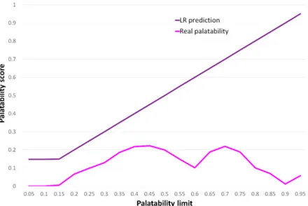
Figure 5.2 compares the performance of the two Machine Learning models embed-ded into the MLBO model. These results are obtained using CPLEX and KNITRO as optimization solvers respectively for the LR-MLBO model and the FCNN-MLBO mode. On the x-axis, we show different values (between 0 and 1) of P limit used in the optimization model. On the y-axis, we show the difference between the real palatability and the palatability predicted by the ML model for the solution obtained by solving the MLBO model.

Figure 5.2: Difference between Real Palatability and Predicted Palatability in both FCNN and LR

This difference is never less than zero due to the fact that the objective function ”pushes” in the direction with lower palatability scores. The amount of each food in the optimal solution and the corresponding value of the objective function are shown in Table A.3 and A.4.

In Figures 5.4 and 5.3, the same type of assessment is shown from a different per-spective. The gray line and the pink line represent the real palatability of the best solutions found at each different P limit s. The blue and violet lines represent the predicted palatability score.

Figure 5.3: Comparison between predicted palatability and real palatability in an FCNN-MLBO scenario.

Figure 5.4: Comparison between predicted palatability and real palatability in an MLBO scenario.

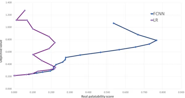
In Figure 5.5, we compare FCNN (blue line) and LR (violet line) defining each solution with its objective value and real palatability score. From an ideal predictive model, we would expect a non-decreasing line that always goes from left to right, but, as we can see, this is not the case in neither of the models studied by us. With the LR-MLBO model, the optimal solutions have much higher objective values compared to those generated by the FCNN-MLBO model. This happens even though with the LR-MLBO the solutions never exceed 0.22 in real palatability score.

Figure 5.5: Comparison between solutions generated with the LR-MLBO and solu-tions generated with the FCNN-MLBO model. Each solution is represented by its real palatability score and objective value.

Even once embedded in the optimization model, the performance of the Neural Network is significantly better than that of Linear Regression. With the LR model, we can solve the MLBO model to global optimality, but because it is not able to clearly describe the space of feasible solutions, it would lead to solutions with no practical meaning. With the FCNN, global optimality is not guaranteed by KNI-TRO, but the approximation of reality is good, especially when compared with the LR.

The worst FCNN performances occur when P limit is around 0.5, and above 0.9. The cause of this error is clearly due to a poor approximation of the Food Basket

Palatability Score function. According to the label definition, the solutions with higher palatability are those closest to the center of the polytope. In other words, the solution with the highest palatability score is the solution whose

P alatabilityComponentg1 value is closest to ±0 for each macro category (whether

they approach zero from negative or positive values). Looking at Table 5.6, we no-ticed a correlation between the performance of the predictive model and the values of P alatabilityComponentg (one for each macro category and calculated as in the

FBG model). The more negative P alatabilityComponentg values are, the greater

the error. It seems that the Neural Network fails to model properly that once the ”center of the polytope” is passed, the palatability score begins to decrease again.

Original MLBO model - Palatability Component per macro category

P limit Cereals&Grains Pulses&Vegetables Oils&Fats Mixed&Blended Meat&Fish&Dairy Error

0.1 125 23.17 12.5 30 20 0.0203 0.2 91.67 1.5 12.5 30 20 0.0464 0.3 49.46 -10.28 12.5 28.10 20 0.0875 0.4 38.17 -27.71 12.5 23.26 17.01 0.1738 0.5 32.71 -35.96 12.5 21.74 15.57 0.2246 0.6 30.58 -33.41 12.24 16.05 12.68 0.2438 0.7 23.91 -22.09 6.59 13.58 10.71 0.1346 0.8 26.30 -11.53 1.33 11.05 8.17 0.0720 0.9 31.77 1.92 -5.78 7.28 5.07 0.2326 0.95 23.96 7.90 -12.49 5.62 4.86 0.4138

Table 5.6: Comparison between P alatabilityComponentg values and the difference

between Predicted and real palatability (Error) in the best solutions found, at dif-ferent P limit in the original MLBO model.

In order to see whether negative values of P alatabilityComponentg critically

affect the performance of the Neural Network, we tested it within the MLBO model modifying the constraint (5.18), which becomes:

minratg + maxratg

2 ≤

X

k∈g

xk≤ maxratg ∀g ∈ G (5.24)

Hence, we bind P alatabilityComponentg to be greater than 0 in each macro

cate-gory. It is still possible to increase the palatability score from 0 to 1, but it is not possible to go beyond the center by continuing in the same direction. The results in Figure 5.6, Figure 5.7, and Table 5.7 show significant improvements in the accuracy of the FCNN model.

1_{P alatabilityComponent}

Figure 5.6: FCNN performance before and after the change of constraint (5.18)

Figure 5.7: Comparison between predicted palatability and real palatability in an FCNN-MLBO model with constraint (5.18) replaced by constraint (5.24)

Modified MLBO model - Palatability Component per macro category

P limit Cereals&Grains Pulses&Vegetables Oils&Fats Mixed&Blended Meat&Fish& Dairy Error

0.1 125.00 23.17 12.50 30.00 20.00 0.0204 0.2 91.67 1.50 12.50 30.00 20.00 0.0465 0.3 40.75 2.28e-07 12.50 25.78 20.00 0.0535 0.4 34.99 2.35e-09 12.50 21.89 15.44 0.0574 0.5 27.50 2.26e-09 9.44 18.60 13.59 0.0291 0.6 18.28 1.24e-07 6.19 15.78 11.29 0.0106 0.7 10.99 5.68e-09 3.23 13.36 9.59 0.0134 0.8 13.69 4.51e-08 0.20 11.03 7.51 0.0350 0.9 14.74 1.30e-09 1.70e-10 3.14 3.30 -0.0289 0.95 4.23 1.09e-09 1.25e-10 1.31 2.9378 0.0220

Table 5.7: Comparison between P alatabilityComponentg values and the difference

between Predicted and real palatability (Error) in the best solutions found, at dif-ferent P limit, with the modified MLBO model.

In Figure 5.6, we see that, in the modified MLBO model, the difference between the predicted palatability and the real palatability is at most equal to 0.0546. In Table 5.7, instead, we see a progressive approach to 0 by P alatabilityComponentg

in all the macro categories when the palatability score increases. We would have ex-pected a similar behavior in the unmodified MLBO model if the FCNN had worked properly.

The same proof was performed with the LR-MLBO model, which resulted in im-pressive results especially for high values of P limit. From 0.7 to 0.9 we have feasible solutions with real palatability scores higher than the predicted ones. This can be a problem in terms of objective value, but it is a good result in terms of feasibility. In Figure 5.8, we can see a comparison between the LR-MLBO model before and after the change of constraint 5.18. The problem, in this case, turns out to be for P limit greater than or equal to 0.95, where the model results infeasible.

Figure 5.8: Comparison between predicted palatability and real palatability in an LR-MLBO model with constraint (5.18) replaced by constraint (5.24)

Also in this case, it is useful to display different solutions, generated by the two modified MLBO models, in terms of real palatability scores and objective values. In Figure 5.9, we show the comparison between the modified LR-MLBO model and the modified FCNN-MLBO model. The optimization model with the Neural Network always has a lower, and therefore better, objective value probably because it is able to better describe the space of feasible solutions allowing the optimization solver to

search in a larger space.

Figure 5.9: Comparison between solutions generated with the modified LR-MLBO model and solutions generated with the modified FCNN-MLBO model. Each solu-tion is represented by its real palatability score and objective value.

The dataset used for model training plays a major role in this error. Indeed, only 1.5% of samples have one or more negative P alatabilityComponentg values.

Therefore, further data generation should be carried out focusing more on solutions with negative P alatabilityComponentg. This requires to modify constraints (5.9)

in the FBG.

5.6.1

Specific Food Basket Generator

For what concerns Neural Networks, another way to improve the performance of predictive models is to insert in the training set solutions computed by MLBO. The iterative logic behind Algorithm 2 requires the use of the MLBO model to generate solutions with different P limit values from 0 to 1. Each solution is associated with its real palatability score calculated with the function (5.12). Once P limit is equal to 1, the solutions and their scores are included in a partially filled dataset for retraining the Neural Network. The initial number of samples in the dataset must be enough to represent the entire population, but not too large, to prevent the new samples from having no effect on the training process. This process is repeated until the accuracy of the embedded Neural Network is considered to be adequate.

Algorithm 2 Recursive execution flow to improve the embedded Neural Network accuracy

Require: pre-trained FCNN

Require: dataset of food baskets. Partial dataset ∈ Rnx26

Require: Palatability limit increment. INCREMENT ∈ R

Require: Limit to the number of iterations. COUNTER LIMIT ∈ R Ensure: Increase in the FCNN accuracy within the MLBO model

1: Counter ← 0 2: do

3: if Counter > 0 then

4: FCNN ← train(FCNN, Partial dataset) 5: end if

6: P limit ← 0

7: while P limit ≤ 1 do

8: solution ← MLBO model(P limit, FCNN)

9: palatability ← Food Basket Palatability Score(P limit,Partial dataset) 10: Save the solution and its palatability in Partial dataset

11: P limit ← P limit + INCREMENT 12: end while

13: Counter ← Counter +1

14: while Counter ≤ COUNTER LIMIT

We used the described FCNN, INCREMENT equal to 0.05 (20 new data points in each iteration), and a Partial dataset with a shape of (40000,26)2_.

The result obtained by executing this algorithm depends on the number of iterations performed. In Figure 5.10, we see how the performance changes as the number of iterations increases. We can see a continuously improving performance until the 20th _{iteration, where it starts to decrease. With 1 iteration (yellow line), we have an}

average improvement of 1.1% in the FCNN accuracy for each P limit value. With 4 iterations (blue line) we have an average improvement of 2.63% with a peak of 7.2% for P limit equals to 0.55. With 20 iterations (red line), the best average im-provement which is around 6.04% with a peak of 26% for P limit equals to 0.55. Even with 50 iterations (green line) the average performance is 5.25% better than the initial FCNN performance, but slightly worse than the performance with 20 interactions.

For high values of P limit, the performance starts to decrease already with 20

iter-2_{The best size of the dataset and the value of INCREMENT are very important decisions that}

ations where the average performance decrease from 0.8 to 0.95 is around 12%.

Figure 5.10: Comparison of embedded FCNNs performance calculated after different iterations of Algorithm 2.

Furthermore, the number of iterations also depends on how the new samples are labeled. If we are working with field data, in order to associate each solution generated by the MLBO model with its palatability score, it is necessary to discuss with the beneficiaries and ask them to provide personal opinions. In view of this, we must consider that it may have high costs and take a long time. However, it would also be possible to perform this process as a natural feedback mechanism to be obtained when the food baskets are delivered to the beneficiaries, before defining the food basket of the successive period.