Breast arterial calcifications on mammograms : deep learning detection for women's cardiovascular risk stratification

Scuola di Ingegneria Industriale e dell’Informazione – MI Dipartimento di Elettronica, Informazione e Bioingegneria

Master of Science in Biomedical Engineering – Ingegneria Biomedica

Breast arterial calcifications on mammograms:

deep learning detection for women’s

cardiovascular risk stratification.

ADVISORS:

Prof. Giuseppe Baselli Dr. Marina Codari, PhD Prof. Francesco Sardanelli

AUTHOR: Maria Giovanna Ienco 893794

II

ABSTRACT

Cardiovascular disease is a major cause of death in women. Up to 20% of all cardiovascular events in women occur without the attendance of conventional risk factors, highlighting a lack in currently cardiovascular risk stratification methods. Breast Arterial Calcifications (BACs), detected on mammograms for breast cancer screening, though extraneous to this primary aim, have attracted the attention of researchers involved in cardiovascular disease prevention. BACs have been suggested as a “potential women-specific cardiovascular risk marker” providing the possibility of transforming the already widespread breast cancer screening program into a double test. The major obstacles to this goal, however, is the lack of a robust method to quantify BACs in mammograms for cardiovascular risk quantification and also adequate automatic support to the further workload asked to radiologists.

In this thesis work, we tackled the latter issue and implemented a deep learning model capable of classifying full breast images according to BACs presence (𝐵𝐴𝐶𝑠+_{) or absence} (𝐵𝐴𝐶𝑠−). We developed a 16-layer convolutional neural network (CNN) using a transfer learning approach. We selected one of the most famous CNN classifiers trained on low resolution natural images, VGG16 net, and customized it in order to classify high-resolution mammograms. We maintained the structure and filters of the original convolutional base and replaced the fully connected part with three new fully connected layers. We selected the optimal number of hidden units of the fully connected layers and the number of convolutional layers to fine-tune. This structure and the relevant hyperparameters were optimized to learn the high-level task-related features while avoiding overfitting. Then, we trained from scratches the fully connected layers, composed by 256, 256 and 1 neurons each, and fine-tuned the last five convolutional layers. To account for class imbalance in the dataset (𝐵𝐴𝐶𝑠+_{prevalence of 10%), we randomly down} sampled the majority 𝐵𝐴𝐶𝑠− _{class until reaching a prevalence of 30%. In addition, a} weighted training approach was used. Data-augmentation was carried out avoid overfitting and also the training epochs were stopped as soon as the validation loss function reached its minimum.

III

We evaluated the resulting architecture and learning strategy performing a 7-fold cross validation using precision, recall, and F1 score as performance metrics. The models showed good performance in terms of precision (range = [0.842-0.950], mean = 0.864 and SD = 0.040) while showing lower recall values (range = [0.433 -0.772], mean = 0.667, SD = 0.132), resulting in a F1 score ranging from 0.653 to 0.840 with mean and standard deviation values equal to 0.744 ± 0.094.

The observation of saliency maps proved the reliability of BAC detection highlighting the ROI of the single BAC or of the most evident BAC of several ones. This allowed us to ascertain the feasibility of transforming global information, such as an image-level annotation, into a local one. Hence, we foresee that the CNN will support the radiologist both by sorting out the few 𝐵𝐴𝐶𝑠+cases and indicating the ROI or ROIs to be closely examined for a future BACs ranking.

Further investigations are needed in order to reduce the number of false negatives before testing the BACs classifier performance on a new independent testing dataset. Despite the obvious need to further improve the model, the results are encouraging and legitimate future studies on the potential role of deep learning automatic BACs detection in the prevention of cardiovascular disease in women.

IV

Sommario

ABSTRACT ... II List of figures ... VI List of tables ... XII Acknowledgments ... XIII

1. Introduction ... 1

1.1 Breast arterial calcifications and cardiovascular risk ... 1

1.2 Digital mammography and BACs ... 7

1.2.1 Image acquisition process and characteristics ... 7

1.2.2 Breast anatomy representation on digital mammograms... 10

1.3 Detection and quantification of breast arterial calcifications on digital mammography ... 16

1.4 Deep learning and breast arterial calcification ... 17

THESIS AIM ... 18

2. Methods ... 19

2.1 Deep learning and Convolutional Neural Networks for binary classification ... 19

2.2 Network-based transfer learning ... 28

3. Protocol ... 31 3.1 System model ... 31 3.2 Dataset ... 32 3.3 Preprocessing ... 35 3.4 CNN architecture building up ... 40 3.4.1 Features extractor ... 41

3.4.2 Fully connected layers... 43

3.4.3 Training strategy ... 45

3.5 Model evaluation ... 51

4. Results ... 52

4.1 CNN architecture and final hyperparameters ... 52

4.1.1 Number of fine-tuned convolutional layer optimization ... 52

4.1.2 Network hyperparameters fine-tuning ... 55

V

4.2 Model validation ... 61

4.3 Saliency maps ... 63

5. DISCUSSION, CONCLUSION AND FUTURE AIMS ... 76

VI

List of figures

Figure 1.1 Top 10 global causes of deaths, 2016. Ischemic heart disease and stroke are the

two major cause of death worldwide [ ... 1

Figure 1.2 Artery wall layers. Arteries are composed of three layers: tunica Intima, tunica

media and tunica adventitia. Tunica intima is the layer in direct contact with the blood and is where the CACs occur. Tunica media is a muscular layer that lets arteries handle the high pressures from the heart. Tunica adventitia is the outermost layer that wraps the vessel. ... 2

Figure 1.3 Healthy and Mönckeberg’s calcific arteries. Cross section of human artery in

normal conditions [a] and with Mönckeberg calcifications in tunica media [b].

[www.sciencephoto.com, www.memorangapp.com] ... 3

Figure 1.4 BACs illustration from a clipped mammogram craniocaudal view.(a) A

mammogram. (b) – (e) Examples of different appearance patterns of calcific arteries on the same mammogram. [from16_{] ... 4}

Figure 1.5 Various appearance patterns of BACs. Breast arterial calcifications in zoomed

mammograms are indicated with yellow arrows. Different appearance is due to different amount of calcium deposition and 2D projection effects. [from16_{] ... 4}

Figure 1.6 Cardiovascular Disease + Breast Cancer screening program [from.8_{] ... 6}

Figure 1.7 Patient undergoing mammography. Patient’s breast is compressed and crossed

by X-rays that attenuated from breast tissues and collected from detector generate the image. [www.teresewinslow.com] ... 7

Figure 1.8 Routine screening mammography standard views. In order: Right CC, Left CC,

Right MLO, Left MLO ... 8

Figure 1.9 Mammogram image with noise. [a] Test image, Poisson Noise [b], Gaussian Nose

[c], Salt and Pepper Noise [d]. [from25_{] ... 9}

Figure 1.10 Breast anatomy[www.webmd.com] ... 10 Figure 1.11 Arterial and venous anatomy of the breast. Paired arteries and veins are found

in the perforating branches of the internal thoracic and lateral thoracic vessels. Intercostal vessels perforate the chest wall musculature to supply deeper parenchymal tissues of the breast [from28_{] ... 11}

Figure 1.12 BACs on right CC and MLO views. Right CC [a], Right MLO [b] views of the same

breast with severe very evident BACs. Not all BACs visible in MLO view (green) are visible in CC view. Signed in red and zoomed [c] BACs visible only in MLO view. ... 11

Figure 1.13 Effect of breast density on digital mammography visualization. From less dense

breast (first on the left) to the densest (last on the right) [www.mayo.edu] ... 12

Figure 1.14 Schematic of the BI-RADS microcalcification distribution descriptors. In order:

Grouped, Regional, Diffuse, Segmental, Linear. [from32] ... 13

Figure 1.15 Examples of microcalcifications on mammogram. Round microcalcifications

diffusely distributed within the breast (little white spots) [a] Regional distribution [b]. [from32_{]... 13}

VII

Figure 1.16 Example of microcalcifications in linear distribution. [from32_{] ... 14}

Figure 1.17 Dermal [a] and milk of calcium [b] calcifications. [from32_{] ... 14}

Figure 1.18 Suture calcifications. Calcification forming knots. Linear or tubular calcifications that may present knots. Common in patient who have undergone radiotherapy.[from32_{] ... 14}

Figure 1.19 Examples of thick linear calcifications. [a] Originating within a duct. Vascular calcifications are present too but is difficult to distinguish between them. [b]Originating in the duct wall. [from32_{] ... 15}

Figure 1.20 Popcorn calcifications. A nodule with coarse calcifications. [from32_{] ... 15}

Figure 1.21 Growth of the number of publications in Deep Learning, Sciencedirect database (Jan 2006-Jun 2017) [from 42_{] ... 17}

Figure 2.1 Artificial intelligence, machine learning and deep learning relationship. [From51_] ... 19

Figure 2.2 Convolutional Neural Network classification pipeline. [From 55 _{] ... 20}

Figure 2.3 How a neuron processes inputs to obtain its output. ... 21

Figure 2.4 Max pooling and Average pooling with a 2x2 filter. [From 59_{]... 23}

Figure 2.5 Binary classification using Sigmoid activation function. ... 23

Figure 2.6 Example of ROC curves. ... 27

Figure 2.7 Learning process of transfer learning. Knowledge transferred from source to the target domain in order to solve the target task. [from 70_{] ... 28}

Figure 2.8 Sketch map of the network-based deep transfer learning. Part of the network trained in source domain with large-scale training dataset is transferred to be part of a new network designed for target domain. [from 70 _{] ... 29}

Figure 2.9 Example of images and labels of ImageNet dataset. [from77_{] ... 29}

Figure 2.10 Different fine-tuning strategies. [a] Train both convolutional and fully connected layers. [b] Train fully connected layers and high-level specific task convolutional layers. [c] Train fully connected layers only. ... 30

Figure 3.1 Example of image and patient labels. CC and MLO views of right breast and MLO view of left breast are labelled as BACs = 1. Left MLO is labelled as BACs = 0 because is not visible in the image. BACs are present in both breasts, so, at the patient level we have a label BACs = 1, bilateral. ... 33

Figure 3.2 Distribution of patients’ age per BACs classes. Histograms of patient distribution according to age of women with and without breast arterial calcifications. ... 34

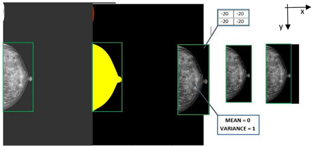
Figure 3.3 Steps involved in data preparation applied to a CC view mammogram. Starting from a 3580x2784 pixels image (first one) in which the breast can be included in an area of 1732x753 pixels (green rectangle), we obtain a 1536x768 pixels image (last one) in which the gray-scale pixels values of the breast have zero mean and variance = 1, the background is isolated (putting all pixels values = -20) and occupy the smaller area possible. It should be noted that the initial image, in addition to the breast, contained a small portion of shoulder (second image, in red) which was removed. ... 37

Figure 3.4 Gray-scale pixels intensities histogram before preprocessing. Image (left) and histogram (right). Red line corresponds to Otsu’s threshold. ... 37

VIII

Figure 3.5 Gray-scale pixels intensities histogram after preprocessing. Whole image

histogram (left), breast pixels histogram (right). ... 37

Figure 3.6 Effect of vertical and horizontal flip in BACs appearance. [a] Original no flipped

patch including BACs [b] Vertical flip [c] Horizontal flip [d] Vertical + Horizontal flip. ... 38

Figure 3.7 VGG16 architecture. Originally designed for the ImageNet database, the image

input size is 224 × 224 and after each Max Pooling layer feature maps dimension is halved. The feature extractor part of the net has as output a tensor of size 7 × 7 x 512, i.e. 512 feature maps of 7 × 7 pixels. ... 41

Figure 3.8 Deep CNN architecture used in Wang et al. BACs detection strategy. [from 39_{] ... 42}

Figure 3.9 Microarchitecture of our convolutional base transferred from VGG16. ... 43

Figure 3.10 Schematic representation of our starting classifier fully connected (FC) part. There are two hidden layers having respectively 1024 and 512 units each, followed by a dropout layer. Black neurons are turned off because of dropout. Output layer consists on one neuron with sigmoid activation function. ... 44

Figure 3.11 CNN architecture obtained stacking VGG16 convolutional base and our designed

fully connected part. ... 45

Figure 3.12 Example of learning rate range estimation. Class-weighted loss function vs

learning rate in Log10 scale is plotted. The minimum learning rate at which the networks already learns is identified by the point in which the loss starts to fast decrease( 10 − 6 ). The maximum boundary is where loss starts to increase ( 10 − 4). ... 48

Figure 3.13 Cosine Annealing schedule. Example of aggressive learning rate schedule where

learning rate starts high and is dropped relatively rapidly to a minimum value near to zero 49 Figure 4.1 Learning rate test. Class-weighted loss function vs learning rate. At each batch update the learning rate is exponentially increased and corresponding loss function is reported. Good learning rates should be values from 10 − 6 and 10 − 4, where the cost function decreases. ... 52

Figure 4.2 Training and validation log-loss function (Binary Cross-Entropy) improving during

training, while adding more convolutional layers to fine-tune. In order: 1, 2, 3, 4, 5, 6 convolutional layers tuned. We can see an initial small improvement from 3, then best performance is reached in model 5. Finally, a little overfitting starts to come from epochs 60 in model 6. ... 53

Figure 4.3 Saliency map of the worst model. Worst model (1 convolutional layer fine-tuned)

saliency map covers the entire breast. ... 54

Figure 4.4 Saliency map of the best model. Best model (5 convolutional layers fine-tuned)

saliency map is overlapped to its mammogram and is concentrated over the BACs ROI. ... 55 Figure 4.5 Distribution of patients’ age per BACs classes in under-sampled database.

Histograms of patient distribution according to age of women with and without breast arterial calcifications after under-sampling of the majority class. ... 56

Figure 4.6 Learning rate test result. Class-weighted loss function vs learning rate. At each

IX

reported. Good learning rates should be values around 10 − 6 and 10 − 3, where the cost function decreases. ... 56

Figure 4.7 Learning rate scheduling after fine-tuning. It corresponds to a truncated Cosine

Annealing schedule, in order to avoid having learning rate too low at which our model would not learn. ... 57 Figure 4.8 Evolution of loss function and metrics during training using a third division (DB3). Cost function, precision, recall and F1 score are reported for each epoch. ... 59

Figure 4.9 ROC curve, best model, third database division (DB3), validation data. ... 59 Figure 4.10 ROC curves by validation data prediction for all 7-fold cross-validation models.62 Figure 4.11 Example of true positive image having severe BACs and its saliency map. (Up,

left) Input 𝐵𝐴𝐶𝑠 + mammogram belonging to validation set, after preprocessing, (up, right) saliency map overlapped to the input image. In red/green the pixels that cause the most change in the output. They correspond to BACs area of the image. (Down, left) Zoomed BACs region. Calcifications are indicated by yellow arrows. (Down, right) Zoomed highlighted BACs regions. The output of the network for this image is equal to 0.9493 (classification threshold equal to 0.5). ... 64

Figure 4.12 Example of true positive image having sparse BACs and its saliency map. (Up,

left) Input 𝐵𝐴𝐶𝑠 + mammogram belonging to validation set, after preprocessing, (up, right) saliency map overlapped to the input image. In red the pixels that cause the most change in the output. They correspond to BACs area of the image. (Down) Zoomed BACs region. BACs are the three white clusters indicated by yellow arrows. The output of the network for this image is equal to 0.9493 (classification threshold equal to 0.5). ... 65

Figure 4.13 Example of true positive having small BACs and its saliency map. (Up, left) Input

𝐵𝐴𝐶𝑠 + mammogram belonging to validation set, after preprocessing, (up, right) saliency map overlapped to the input image. In red the pixels that cause the most change in the output. They correspond to BACs area of the image. (Down) Zoomed BACs region. BACs are white pixels indicated by yellow arrows. The output of the network for this image is equal to 0.9964 (classification threshold equal to 0.5). ... 66

Figure 4.14 Example of true positive image having linear one side BACs and its saliency map.

(Up, left) Input 𝐵𝐴𝐶𝑠 + image belonging to validation set, after preprocessing, (up, right) saliency map overlapped to the input image. In red the pixels that cause the most change in the output. They correspond to BACs area of the image. (Down) Zoomed BACs region. BACs are white pixels between the two yellow arrows. The output of the network for this image is equal to 0.9987 (classification threshold equal to 0.5). ... 67

Figure 4.15 Example of true positive image with dense breast and its saliency map. (Up,

left) Input 𝐵𝐴𝐶𝑠 + mammogram belonging to validation set, after preprocessing, (up, right) saliency map overlapped to the input image. In red the pixels that cause the most change in the output. They correspond to BACs area of the image. (Down) Zoomed BACs region. BACs are white pixels indicated by yellow arrows. The output of the network for this image is equal to 0.9968 (classification threshold equal to 0.5). ... 68

X

Figure 4.16 Example of true positive image having and its saliency map. (Up, left) Input

𝐵𝐴𝐶𝑠 + image belonging to validation set, after preprocessing, (up, right) saliency map overlapped to the input image. In red the pixels that cause the most change in the output. They correspond to BACs area of the image. (Down) Zoomed BACs region. BACs are white pixels indicated by yellow arrows. The output of the network for this image is equal to 0.9705 (classification threshold equal to 0.5). ... 69

Figure 4.17 Example of true positive having benign calcifications and its saliency map. (Up,

left) Input 𝐵𝐴𝐶𝑠 + image belonging to validation set, after preprocessing, (up, right) saliency map overlapped to the input image. In red the pixels that cause the most change in the output. They correspond to BACs area of the image. (Down, left) Zoomed BACs region. Very severe BACs indicated by yellow arrows. (Down, right) Zoomed region containing round benign calcifications. The prediction is not affected from the presence of other types of calcifications. The output of the network for this image is equal to 0.9997 (classification threshold equal to 0.5). ... 70

Figure 4.18 Example of false negative image and its saliency map highlighting BACs region.

(Up, left) Input 𝐵𝐴𝐶𝑠 + image belonging to validation set, after preprocessing, (up, right) saliency map overlapped to the input image. In red the pixels that cause the most change in the output highlighting the They are localized in an area without BACs. (Down) Zoomed highlighted region. The output of the network for this image is equal to 0.400 (classification threshold equal to 0.5). ... 71

Figure 4.19 Example of false negative image and its saliency map partially highlighting BACs

region. (Up, left) Input 𝐵𝐴𝐶𝑠 + image belonging to validation set, after preprocessing, (up, right) saliency map overlapped to the input image. In red/blue the pixels that cause the most change in the output. They are localized in three different area of the breast. In the first, the most highlighted region in red, zoomed in the green rectangle (down, left)

corresponds to a BACs region. The second one, in highlighted in blue e zoomed in the yellow rectangle (down, middle) was signed from our human reader as a dubious region. The third region contains absolutely no BACs. The output of the network for this image is equal to 0.4699 (classification threshold equal to 0.5). ... 72

Figure 4.20 Example of false negative image and its saliency map highlighting no BACs

region. (Up, left) Input 𝐵𝐴𝐶𝑠 + image belonging to validation set, after preprocessing, (up, right) saliency map overlapped to the input image. In red the pixels that cause the most change in the output highlighting a region not including BACs. (Down) Zoomed highlighted region. The output of the network for this image is equal to 0.1569 (classification threshold equal to 0.5). ... 73

Figure 4.21 Example of false positive image and its saliency map. (Up, left) Input 𝐵𝐴𝐶𝑠 −

image belonging to validation set, after preprocessing, (up, right) saliency map overlapped to the input image. In red the pixels that cause the most change in the output. They are localized in an area without BACs. (Down) Zoomed highlighted region. This image has an output of the output neuron equal to 0.6635 (classification threshold equal to 0.5). ... 74

XI

Figure 4.22 Examples of true negative images and their saliency maps. The outputs of the

net having these images as inputs are respectively 0.0284 and 0.04725 ... 75

Figure 5.1 Example of breast arterial calcification correctly detected in presence of several

high intensity objects with tubular morphology... 79

Figure 5.2 Example of breast artery with multiple calcified segments. Despite the large

extension of BAC segments along the vessel, the saliency map shows only one bright spot as a result of the binary classification task performed the developed convolutional neural network. ... 81

XII

List of tables

Table 2.1 Confusion matrix. ... 25

Table 3.1 Acquisition systems and images properties. ... 32

Table 3.2 Labels per patient. Number of patients with or without breast arterial calcifications in our dataset. ... 34

Table 3.3 Labels per image. Number of images labelled as presenting BACs or not in our dataset. ... 34

Table 4.1 Labels per patient. Number of patients with or without breast arterial calcifications in our dataset. ... 52

Table 4.2 Labels per image. Number of images labelled as presenting BACs or not in our dataset. ... 52

Table 4.3 Labels per patient after resampling. Number of patients with or without breast arterial calcifications in our resampled dataset used to fine-tune hyperparameters. ... 55

Table 4.4 Labels per image after resampling. Number of images labelled as presenting BACs or not in our resampled dataset used to fine-tune hyperparameters. ... 56

Table 4.5 Specifications of models trained in manual grid-search. Hidden units (1) and (2) refer respectively to the number of neurons of the first and second fully connected layers. Conv. Layers is the number. In green the best configuration. ... 57

Table 4.6 Metrics evaluated for each parameter combinations model. Precision, Recall, F1 score, Area Under the ROC Curve (ROC AUC) calculated on the validation set, for each model is shown. Epoch refers to the epoch in which the validation loss function value was minimum, at which point we saved the model weights as the optimal ones. Model 5 is highlighted in green, since it displayed the best performances in both DB1 and DB2 validation datasets. ... 58

Table 4.7 Metrics calculated on validation data. ... 59

Table 4.8 Confusion matrix of validation data predictions. ... 59

Table 4.9 Final CNN architecture. ... 60

Table 4.10 7-fold cross-validation results for training set. ... 61

Table 4.11 7-fold cross validation compressive result on training set. ... 61

Table 4.12 7-fold cross-validation results for validation set. ... 61

XIII

Acknowledgments

I would like to thank those who made the success of this thesis possible and those who supported me in these months of hard work.

I thank the Politecnico di Milano for giving me the theoretical foundations and the tools necessary to face such a complex problem with cutting-edge methods.

I thank Prof. Baselli for having followed me with constancy and patience and for giving me the opportunity to exploit his precious experience.

I thank Marina, who throughout the thesis period has been my fixed point of reference, always ready to give me the right advice. I thank you for the passion for your work that I was allowed to share with you.

Finally, I want to thank Prof. Sardanelli and all the research team of the IRCCS Policlinico San Donato, without them, this work would not have existed. Thank you for your time and sharing your knowledge with me.

1

1. Introduction

1.1 Breast arterial calcifications and cardiovascular risk

Cardiovascular disease (CVD) is the most common cause of death overall, causing the loss of around 7.9 million men and women each year. According to the World Health Organization, the number of deaths is destined to rise to 22.2 million by 20301_{. The 85%}

of CVD demises are the consequences of strokes and ischemic heart diseases, which occupy the first two places in the ranking of global causes of deaths, the top 10 shown in

Figure 1.1.

Figure 1.1 Top 10 global causes of deaths, 2016. Ischemic heart disease and stroke are the two major cause of death worldwide [www.who.int]

CVD constitutes a major healthcare problem that requires new prevention and risk stratification strategies, especially for women2_{. Many women with conventional risk}

factors have never experienced coronary heart diseases3_{, while up to 20% of all coronary}

events in women occur without the attendance of major risk factors4_{. These facts suggest}

sex-specific risk factors or cofactors (like pregnancy complications, oral conception, menopausal therapies, hormonal fertility5_{) not included in the actual CVD risk assessment.}

2

One of the most widely used CVD risk scores is the Framingham Risk Score (FRS), developed in 20086_{. The FRS is a sex-specific algorithm that estimates the risk of}

manifesting clinical CVDs in the next 10 years. Age, sex, total cholesterol level, high-density lipoprotein, systolic blood pressure, smoke, diabetes, hypertension and other known vascular diseases are the FRS covariates. Current guidelines recommend the inclusion of also sex and ethnicity into the calculation7_{, however the predictive value of}

risk scores based only on demographic and life-style factors is still poor. Actually, the lack of reliable, effective screening modalities remains and constitutes one of the major barriers to improve CVD outcomes in women8_{. Among noninvasive imaging biomarkers, coronary}

artery calcium (CAC) score is the most potent marker of subclinical cardiovascular disease and has been demonstrated to enhance risk prediction in women9_{. American and European}

guidelines recommend it to improve cardiovascular risk assessment in asymptomatic individuals with low-intermediate risk10_{. CACs are calcifications of the tunica intima (inner}

layer) (Figure 1.2) of the coronary arteries, vessels that wrap around the entire heart for suppling it. CACs are the results of the atherosclerotic process, an inflammatory process leading to lipid deposits and luminal narrowing11_{. CACs can be seen on a non-contrast}

chest computed tomogram (NCCT). However, a widespread CAC screening program, similar to mammography for breast cancer prevention, would expose women to excessive radiation, with a too unspecific indication. Furthermore, in some countries such as United States, assurance companies don’t cover the costs of such screening.

Figure 1.2 Artery wall layers. Arteries are composed of three layers: tunica Intima, tunica media and tunica adventitia. Tunica intima is the layer in direct contact with the blood and is where the CACs occur. Tunica media is a muscular layer that lets arteries handle the high pressures from the heart. Tunica adventitia is the outermost layer that wraps the vessel.

3

Breast Arterial Calcifications (BACs) are localized calcific depositions in the tunica media of breast arteries and are a manifestation of the Mönckeberg’s medial calcific sclerosis, notably different from atherosclerotic process involved in CACs formation12_.

Calcifications are diffuse within the tunica media of medium and small muscular arteries involving nonocclusive circumferential thickening (Figure 1.3) which results in stiffer, less compliant vessels.

Figure 1.3 Healthy and Mönckeberg’s calcific arteries. Cross section of human artery in normal conditions [a] and with Mönckeberg calcifications in tunica media [b]. [www.sciencephoto.com, www.memorangapp.com]

BACs prevalence varies depending on population age and comorbidities. In screening mammography population-based cohort studies it is reported to range from 10% to 12%. However, BACs prevalence can reach 70% in women aged 70 years or more in women with chronic kidney diseases1314_.

BACs are easily recognizable on breast cancer screening mammograms, where they appear as linear, parallel opacities on both sides of the vessel lumen (Figure 1.4). which justifies the term of “tram-track appearance”, in particularly evident BACs15_{. However,}

BACs can assume several aspects: involving vessels, or only one side of them, or can also appears as small intense dots superimposed on the artery lumen (Figure 1.5).

4

Figure 1.4 BACs illustration from a clipped mammogram craniocaudal view.(a) A mammogram. (b) – (e) Examples of different appearance patterns of calcific arteries on the same mammogram. [from16_]

Figure 1.5 Various appearance patterns of BACs. Breast arterial calcifications in zoomed mammograms are indicated with yellow arrows. Different appearance is due to different amount of calcium deposition and 2D projection effects. [from16_]

5

From an oncological perspective, BACs do not represent a sign of breast cancer and for this reason are ignored or barely reported as present/assent. Nevertheless, BAC become more interesting for the research community as a “potential women-specific CVD risk marker17_{”. Several studies investigated the association among BAC seen on breast cancer}

screening mammograms, traditional cardiovascular risk factors and CVD events As reported on a recent meta-analysis published by Hendriks et al. 13_{, age and diabetes are}

directly associated with BACs prevalence while no associations were found with other CVD risk factors such as obesity, hypertension and dyslipidemia. BACs are instead associated with an increase of CVD events suggesting that “medial arterial calcifications might contribute to CVD through a pathway distinct from the intimal atherosclerotic process13_”.

In a study18 _{performed on a retrospectively selected sample of 292 women who underwent}

both mammography and NCCT, Margolies et al. investigated the association between CACs and BACs assessed using quantitative scores (0 to 12). They compared them with FSR and the 2013 Cholesterol Guidelines Pooled Cohort Equations (PCE). Their results showed that BACs are associated with increasing age (p<0.001), hypertension (p=0.007) and chronic kidney disease (p<0.0001) and all BACs variables are predictive of the CACs score (p<0.0001). BACs>0 had area under the curve of 0.73 for identification of women with CACs>0, equivalent to both FSR (0.72) and PCE (0.71). For the identification of high-risk CACs (score from 4 to 12) BACs>0 increased the area under the curve curves for FRS (0.72 to 0.77; p=0.15) and PCE (0.71 to 0.76; p=0.11). BACs resulted to be superior to standard cardiovascular risk factors and to be strongly quantitatively associated with CACs.

In this light, we should exploit current breast cancer screening mammographic program to obtain a double test. Mammograms for breast cancer screening could be further exploited for CVD prevention without any additional radiation exposure or cost. Bui et al.8

in their review wrote: “ At the very last, we strongly believe that the presence of BAC should initiate a personalized patient-provider discussion surrounding lifestyle changes and targeted medical therapies for prevention of cardiovascular disease or consideration for referral for cardiovascular risk assessment by specialist”. Their proposal, anticipated

6

and shared by many researchers actively involved in the cause, is reported schematically in Figure 1.6

Figure 1.6 Cardiovascular Disease + Breast Cancer screening program [from.8_]

Harnessing the full potential of digital screening mammograms can enhance prevention of the two leading causes of death in women, namely CVD and breast cancer. Still, this ambitious goal lacks two important points: a) so far, it doesn’t exist a robust quantitative or semi-quantitative scale to quantify BAC load, to stratify women’s CV risk

19_{; b) an AI or deep learning (DL) tool to assist radiologist in this further diagnostic effort.}

The latter issue is focused by this thesis and is motivated by the difficulty of BACs detection, also considering its difficulty even to expert radiologists, which could distract them from the primary cancer prevention purpose. Indeed, the above introduction, has clearly illustrated such problem, since BACs: a) can be significant even if a single lesion was radiologically detectable; b) have variable aspects and dimensions; c) their localization in the breast is unpredictable.

Therefore, it was decided to provide a DL CNN tool, trained, validate, and possibly tested on a sufficiently large database of mammograms annotated as BACs positive (𝐵𝐴𝐶𝑠+) or negative (𝐵𝐴𝐶𝑠−). Currently 293 𝐵𝐴𝐶𝑠+and 2575 𝐵𝐴𝐶𝑠− images were available, to be increased in the near future. Accordingly, the CNN outcome is limited to the indication of a highly probable presence of one or BACs, avoiding the specific analysis and waste of radiologist’s time on the prevalent 𝐵𝐴𝐶𝑠− _{cases, since the demographic} prevalence in women undergoing mammographic screening ranges from 10% to 12% . Nonetheless, limited localization of at least the prominent BAC lesion is given by the CNN decision heat map.

7

1.2 Digital mammography and BACs

1.2.1 Image acquisition process and characteristics

Mammography is a specific type of two-dimensional (2D) breast imaging that uses low-energy X-rays, usually around 30 kVp20_{. It is mainly used for the detection of breast}

cancer at early stage ahead of palpable breast nodules. During a mammogram, a patient’s breast is placed between two plastic plates and compressed to reduce projection thickness as much as possible. Then, an X-ray machine produces a burst of X-rays that passes through the breast to a detector located on the opposite side (Figure 1.7).

Figure 1.7 Patient undergoing mammography. Patient’s breast is compressed and crossed by X-rays that attenuated from breast tissues and collected from detector generate the image. [www.teresewinslow.com]

In digital full field mammography, the processes of image acquisition, storage/retrieval, and display are separated. Acquisition is often performed using a Flat Panel Detector (FPD) made by a high-resolution matrix of light sensitive elements (charge coupled devices or thin film transistors), each of which captures and image pixel. Conversion from X-rays to visible light is performed by a thin scintillation layer (frequently, thallium activated cesium iodide, CsI: Tl)). Scatter suppression is normally enhanced by a collimation grid overlapped to the FPD. The natively digital image is output by the FPD, stored on disk, and displayed either on a high-resolution radiological screen or on a film by laser printing. Quantization of signal levels occurs in the analog-to-digital conversion process, during the read-out of the FPD, since the FPD elements are spatially discrete pixels but still storing analogic values in the form of electrical charge. The number

8

of bits digitization must be adequate to represent subtle difference in X-ray attenuation by tissue over a wide dynamic range of X-ray exposure21_.

However, the method of ex-post digitalization of analogic fluorescence memory plates is still in use, due to the higher flexibility in resolution and precision settings. In place of an RX film, a memory plate is used. This detector, in place of photosensitive AgCl has a thin layer of fluorophore that does not immediately generate fluorescence, but stores energy for a while. Thus, only the stimulation by a laser beam in the dark room of a laser scanner is able to cause the stimulated fluorescence. In this way, the image stored in the memory plate is read-out scanning it by the laser beam, sensing and digitalizing the emission at each spot. Differently from FPDs, resolution and precision are hence determined by the read-out phase settings.

Digital mammograms are high resolved images but there is not an absolute standard for spatial resolution. The minimum pixel size on the detector required for digital mammography has been subject for debate. The size of the pixel element on currently available detectors ranges between 50 µm and 100 µm. Digital mammograms are usually represented with 4096 gray levels using 12 bits per pixel22_{, but gray level resolution can}

change between vendors too. The routine screening mammography includes the acquisition of two standard views for each breast, namely, craniocaudal (CC) and mediolateral oblique (MLO) views, thus providing four images per patient (as shown in Figure 1.8).

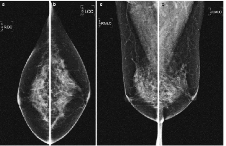
Figure 1.8 Routine screening mammography standard views. In order: Right CC, Left CC, Right MLO, Left MLO

9

Image quality is affected by the size, shape and X-ray absorption properties (i.e., density) of the imaged breast. In addition, X-ray beam quality, geometric un-sharpness and contrast, resolution, detector system noise, and scatter suppression are not standardized in the market and can add additional variability23_.

Salt and Pepper, Gaussian and Poisson Noise are the main types of noises that affect mammogram images. They are the result of different image acquisition processes but altogether can create problems to the fine analysis and interpretation of the breast image leading to wrong diagnosis. On mammographic image formation process the modulation transfer function (Amplitude of Fourier transform of the point spread function, PSF) adds a blurring which degrades the image spatial resolution. The core element is the focal spot size in the X-ray tube anode, the sized of which approximately gives the FWHM size of the PSF. Therefore, in mammographers the focal size is about a half of other X-ray imagers ranging from 0.3 to 0.6 mm. Quantum noise comes from acquisition system low-counts X-ray photons and can be described by a Poisson distribution, which causes random errors called Poisson Noise (Figure 1.9 [b]) and is the predominant noise in digital mammograms, given the very low exposure. The electronic noise from digital mammography systems can be modeled as an additive Gaussian noise (Figure 1.9 [c]). Salt and pepper noise is the consequence of sudden changes of image signal and is frequent in digital imaging systems when the conversion of FPD data to image is quicker24_{. This}

phenomenon changes some pixels with minimum or maximum intensities randomly, appearing as black and white dots in the image (Figure 1.9 [d]).

[a] [b] [c] [d]

Figure 1.9 Mammogram image with noise. [a] Test image, Poisson Noise [b], Gaussian Nose [c], Salt and Pepper Noise [d].[from25_]

10

1.2.2 Breast anatomy representation on digital mammograms

The breasts are complex structures located on the anterior thoracic wall, in the pectoral region, overlying the chest muscles. Each breast is mainly composed of glandular tissue specialized in milk production, supportive tissue (dense breast tissue), fatty tissue (non-dense breast tissue) but also contains lymph vessels, lymph nodes and blood vessels (Figure 1.10). The glandular part named parenchyma includes 15 to 20 sections called lobes arranged like the petals of a daisy. Each lobe has many smaller structures called lobules where milk is produced. Lobes and lobules are linked by tiny tubes called ducts conveying milk to the nipple. There are not muscles in the breast, but they lie between the breast and the chest.

Figure 1.10 Breast anatomy[www.webmd.com]

The arterial supply to the breast (Figure 1.11) is primarily derived from branches of the internal thoracic artery (a branch of the subclavian artery), intercostal arteries, and the lateral thoracic artery. From the surface, arterial branches of the internal and thoracic arteries arborize across the breast and go deep into the breast parenchyma26_{. The venous}

anatomy of the breast parallels the arterial anatomy in the deep breast tissues but superficially the venous anatomy is variable and differs from arterial location27_.

11

Figure 1.11 Arterial and venous anatomy of the breast. Paired arteries and veins are found in the perforating branches of the internal thoracic and lateral thoracic vessels. Intercostal vessels perforate the chest wall musculature to supply deeper parenchymal tissues of the breast [from28_]

The variability of the breast vascular system visualization given by the variable number of branches of each principal vessel, variable position and the overlap in the 2D mammograms projection, complicates the BACs detection. Combining the two views per breast radiologists can inspect the complex vascular anatomy, which cannot be visible by a single projection thus enhancing BAC detection29 _{(Figure 1.12).}

[a] [b] [c]

Figure 1.12 BACs on right CC and MLO views. Right CC [a], Right MLO [b] views of the same breast with severe very evident BACs. Not all BACs visible in MLO view (green) are visible in CC view. Signed in red and zoomed [c] BACs visible only in MLO view.

12

The mammographic image brightness and contrast also depend on breast density, which decreases with aging. On a mammogram, non-dense breast tissue appears dark and transparent instead dense breast tissue appears as a solid white area, which makes it difficult to see through (Figure 1.13). Radiologists quantify breast density as the ratio between non-dense and dense tissues. Usually, there is an inverse relationship between patient age and mammographic breast density30_.

It has been found that women with dense breasts have a four to six higher risk of late breast cancer detection compared with women having no glandular tissue or with little glandular tissue, within the same age range. It is a common belief that one of the reasons could be the masking of lesions by the overlying breast dense tissue making difficult for radiologists detect cancer on early stage 31_{. In the same way, BACs can be covered from dense tissue,}

thus being not visible in mammography. Fortunately, BACs hidden in one view are often shown up in the other one.

Figure 1.13 Effect of breast density on digital mammography visualization. From less dense breast (first on the left) to the densest (last on the right) [www.mayo.edu]

Moreover, BACs are not the only type of calcifications that can be seen on digital mammograms. Hernández et al. provide an exhaustive description of calcifications categories according to BI-RADS 5th _{edition in their article}32_{. They report that many of}

these calcifications have a benign origin such in the case of response of inflammatory disease of ducts or coarse calcifications in benign nodules. Other calcifications can be the caused by malignant disease or high-risk lesion. Since our purpose in this section is to give

13

an idea of disturbing factors in BAC detection, we will just show some examples among the cases that they reported without specifying and going deep into benignant/malignant origin. They provide a first description based on microcalcification distribution showed in

Figure 1.14. Every configuration could be a confounding source in BACs detection (for

example in the case of a calcified dot that appears in mammography superimposed on a vase but in reality they are located in different panels), but particularly in linear distribution the calcific deposition suggests a deposits within a duct but in some cases is not too easy distinguish between vessels and milk’s ducts (Figure 1.16). They talk about also dermal, milk of calcium (small particles of calcium oxalate settling within saccular dilatations of the terminal duct lobular units), nodular, intraductal calcifications and here we report some images as examples.

Figure 1.14 Schematic of the BI-RADS microcalcification distribution descriptors. In order: Grouped, Regional, Diffuse, Segmental, Linear. [from32]

[a] [b]

Figure 1.15 Examples of microcalcifications on mammogram. Round microcalcifications diffusely distributed within the breast (little white spots) [a] Regional distribution [b]. [from32_]

14

Figure 1.16 Example of microcalcifications in linear distribution. [from32_]

[a] [b]

Figure 1.17 Dermal [a] and milk of calcium [b] calcifications. [from32_]

Figure 1.18 Suture calcifications. Calcification forming knots. Linear or tubular calcifications that may present knots. Common in patient who have undergone radiotherapy.[from32_]

15

[a] [b]

Figure 1.19 Examples of thick linear calcifications. [a] Originating within a duct. Vascular calcifications are present too but is difficult to distinguish between them. [b]Originating in the duct wall. [from32_]

16

1.3 Detection and quantification of breast arterial calcifications on

digital mammography

Achieving an effective method of BACs assessment is not an easy task. Many scientists in the literature have tried to make their own version, but none of them has proved to be eligible as standard method to be used by clinicians. One of the biggest problems is surely the heterogeneity in BACs appearance in mammographic images. They can have different appearance patterns (tubular, single or parallel structures, little bright spots) and added to the topological complexity and vessels overlapped on two-dimensional projections make both BACs identification and quantification real challenges33_.

Many studies described BACs on a dichotomous scale3435 _{, other in a semi-quantitative}

scale1836 _{but there are few cases of quantitative scale, too. Part of quantitative methods are}

based on manual segmentation measure37 38 _{, which is time consuming and operator}

dependent. Aiming at including BAC assessment within a screening test, it is very important to minimize the reporting time and, even more important, operator-dependency of the manual segmentation process2_.

Recent studies have focused on the realization of automatic BAC segmentation methods, addressing operator-dependency by using multiple readers to establish the reference standards3339_{. In some case, BACs are segmented, just to exclude them from the}

microcalcification detection for breast cancer diagnosis. In this light, several algorithms have been proposed for automated BAC detection. For example, Mordang et al.40 _{used a}

GentleBoost classifier to remove BACs from mammograms in microcalcification detection by a set of manually designed features obtaining a reduction of the number of false positives per case by 29% on average. In another study, Cheng et al.16 41 _{developed a}

twosteps fully automatic algorithm. In the first step with a random walk-based tracking algorithm they found BAC paths, then with the second step based on a linking algorithm they grouped BAC paths into BACs. Their proposed method was tested on 40 mammograms and achieved performance of 93.8±1.3% in sensitivity and 84.7±3.9% in specificity.

17

Despite these efforts, the automatic BAC detection is far from clinical deployment. There is the need to go deeper and invest in a method that should: i) account for the diversity in shape, location, appearance and prevalence of BACs; ii) be insensitive to the variability of different machines; iii) not suffer the influence of other complex or abnormal structures of the breast that appear intense in mammograms; and iv) eliminate operator dependence.

1.4 Deep learning and breast arterial calcification

From the first appearance in 200642 _{as a new field of research field within machine}

learning, Deep Learning (DL) algorithms have been extensively applied in image analysis

43 44_{. The versatility of this approach has allowed to tackle a wide range of task, ranging}

from pattern classification and detection in natural images45_{, to a system to screen}

coronavirus (COVID-19) disease pneumonia in the currently worldwide spread of pandemia46_.

Figure 1.21 Growth of the number of publications in Deep Learning, Sciencedirect database (Jan 2006-Jun 2017) [from 42_]

Convolutional Neural Network (CNN) is one of the successful and popular deep learning techniques to perform image classification allowing to outperform traditional classifier in several cases47_{.The main strength of CNN is that it can automatically perform}

both the feature extraction and classification tasks by a fully data-driven strategy, so that there is no need for manual feature extraction and selection48_.

18

Due to their peculiar characteristics CNNs have been applied also to BACs detection. In a recent study, Wang et al.39 _{investigated the potential of deep learning for BACs}

detection on mammograms. To date, and to the best of our knowledge, this study is the only documented case of deep learning application for BAC detection. In their study, the authors developed a 12-layer convolutional neural network to discriminate BACs from non-BACs pixels using a pixelwise, patch-based procedure for BACs-detection and segmentation. They asked to expert radiologists to manually provide the boundaries of BACs in mammograms, then they extracted from these images a number P of batches of size 95×95 pixels from BAC-regions and a number P of batches of same size from non-BAC regions. The image patches were fed to the CNN trained to provide the probability of the central pixel to belong to the BACs class or not. They tried to address the operator-dependency asking multiple readers to establish the presence and location of BACs and using the boundaries provided by the most experienced reader. Known that the determination of BACs boundary is considerably more subjective than BACs location and they used segmentations provided from only one reader to train the net, as a consequence this approach is not fully operator independent.

THESIS AIM

The first aim of this thesis is to implement a binary classifier of mammographic images to discriminate the presence/absence of BACs using pretrained CNN; i.e. the manual annotation used for training, validation, and possibly testing and the trained CNN output is dichotomic: positive (𝐵𝐴𝐶𝑠+) to the presence of at least one BAC, negative (𝐵𝐴𝐶𝑠−), no BAC detected. The second purpose is to verify the support to manual segmentation of the main BAC (or BACs) offered to the radiologist in 𝐵𝐴𝐶𝑠+ _{cases, thanks to the focus on} a limited breast region provided by the CNN heat/saliency map.

Training a CNN on a database with whole image annotation, i.e. the single dichotomous annotation 𝐵𝐴𝐶𝑠+_{/𝐵𝐴𝐶𝑠}− _{is the proposed strategy expressly chosen to} reduce operator-dependency and to obtain a less biased result. Here we want to investigate the feasibility of the proposed method and find the network structure and transfer-learning approach that best suits the problem.

19

2. Methods

2.1 Deep learning and Convolutional Neural Networks for binary

classification

Machine learning (ML) is a term introduced by Arthur Samuel in 1959 to describe an artificial intelligence (AI) subfield 49_{. ML includes all those approaches that allow}

computers to learn from data without being explicitly programmed. Deep learning (DL) has emerged as one of the most promising machine learning techniques (Figure 2.1). DL methods belong to representation-learning methods with multiple levels of representation, which process raw data to perform classification or detection tasks50 _.

Figure 2.1 Artificial intelligence, machine learning and deep learning relationship. [From51_]

Neural network architecture is structured in layers composed of interconnected nodes. This structure mimics the interconnection of natural neurons, which perform summation of inputs each weighted by the relevant synapsis strengths, next firing if and only if a threshold is reached. So, each node of the artificial neural network (ANN) executes a weighted sum of the input data that are subsequently passed to a highly nonlinear activation function. Weights are dynamically optimized during the training phase, similar to the long-term-potentiation/depotentiation of natural synapses. We can distinguish between three different kinds of layers: the input layer, which receives input data; the hidden layer(s), which are in charge to extract the patterns within the data; and the output layer, which provides the processing results. Deep neural networks were introduced to improve on the performance of conventional ANN adding many hidden layers, which characterize the depth of the network. In deep learning multiple linear and non-linear processing units are arranged in deep architectures to model high level information abstraction present in the

20

data52_{. There are several deep learning techniques including auto-encoders, restricted}

Boltzmann machines, deep belief networks53 _{and deep convolutional neural networks}

(CNNs).

CNNs are feedforward networks in which the information flow takes place in one direction only. Their architecture is biologically inspired by the visual cortex of the human brain, which consists of alternating layers of simple and complex cells54_{. It is worth}

recalling that convolution is the main signal or image processing step, which simply consists of a scalar product (point-by-point multiply and overall summation) of data (in this case the CNN input or the output of the previous layer) with a set or fixed coefficients (in this case, the synaptic weights). Most feature extraction methods (Fourier, filtering, cross-correlation, matched filtering, texture analysis, etc.) are actually based on convolutions. CNNs architectures may strongly vary among different tasks but are generally composed by convolutional and pooling (or subsampling layers) steps grouped in blocks stacked on top of each other to form a deep model. Interestingly, pooling and next un-pooling implements the multiscale approach, which in the traditional signal/image processing is implemented by wavelet techniques, with self-similar convolutions done at different scales. Stacked modules are always followed by one or more fully connected layers, as in standard feedforward neural network. In Figure 2.2 an illustration is shown of a most popular basic CNN architecture for a toy image classification task provided from Rawat et al. in their review53_{. An input image is passed to the network and is processed}

through different convolutional and pooling stages. Then, representations of image content (i.e. extracted image features) are processed by one or more fully connected layers. The last fully connected layer (output layer) provides an estimate of the input image class label.

21

Convolutional layers

The Convolutional base of a CNN works as feature extractors. It aims at learning the feature representations of their input images. The neurons in the convolutional layers are organized in feature map and each neuron has a receptive field, which is connected to a neighborhood of neurons in the previous layers via a set of weights arranged in a matrix called kernel. Inputs are convolved with the kernel weights to compute new feature maps. Each convolved result is then summed to a bias value and sent through a non-linear activation function that typifies the neuron and allows the extraction of nonlinear features (Figure 2.3).

Figure 2.3 How a neuron processes inputs to obtain its output.

Each feature map is the results of the application of a specific kernel, nevertheless the same convolutional layer contains multiple filtering kernels thus representing a high-dimensional feature space. Each neuron is characterized by a specific activation function. Traditional activation functions are the sigmoid and hyperbolic tangent functions defined, respectively, as:

𝑓(𝑥) = 1

1+𝑒−𝑥 Equation 2.1 , 𝑓(𝑥) = tanh⁡(𝑥) Equation 2.2 Where 𝑓 is the neuron output as a function of its input of 𝑥 (convolution result plus bias). Sigmoid activation function looks like a S-shape (Figure 2.5) and its output ranges between 0 and 1. We can distinguish three regions: zero-saturation region, linear region and one-saturation region.

22

Recently, rectified linear units (ReLU) and their variants became popular, due to their simplicity and efficiency. Introduced by Nair and Hilton in 2010 56 _{the ReLU is a piecewise}

linear function defined as:

𝑓(𝑥) = max⁡(𝑥, 0) Equation 2.3

i.e. it retails only the positive part of the activation by reducing the negative part to zero, promoting faster computations. It was demonstrated that ReLU leads to faster convergence

56 _{and not to suffer from the vanishing gradient problem, in which the lower layers have}

gradients near to zero because of the saturation of higher layers, in the back-propagation algorithm 57_{. ReLU shows possible disadvantages during the optimization process since}

the gradient is zero when the unit is not active (the derivative of the ReLU is 1 in the positive part and 0 in the negative part) 58 _{.This may fall to sub-optimal solutions of training}

where not activated neurons will be never retrieved. Thus, ReLU can lead to slow convergence of the training process when gradients are constant near to zero. Maas et al.

58 _{tried to solve this problem by introducing Leaky Rectified Linear Units (Leaky ReLU),}

a variant of traditional ReLU that allows for small nonzero gradients when the unit is not active. Leaky ReLU is defined as follow:

𝑓(𝑥) = max(𝑥, 0) + ⁡𝜆⁡min⁡(𝑥, 0) Equation 2.4 Where λ is a predefined parameter within the range (0,1).

Pooling layers

Pooling layers have the purpose of reducing the feature maps spatial resolution and achieve spatial invariance to input scale changes and distortions. Pooling create partitions of the input image into a set of non-overlapping sub-regions and presents as output only one value per partition, calculated according to a specific rule. Figure 2.4 represents two of the most used pooling types: Max pooling and Average pooling. Max pooling aggregation layers propagate the maximum value within a receptive field to the next layer, while Average pooling ones propagate the average value. Max pooling followed by the activation function is similar to a non-exclusive OR operations (alias, winner-takes-all), while Average pooling has a smoother, more linear behavior.

23

Figure 2.4 Max pooling and Average pooling with a 2x2 filter. [From 59_]

Fully connected layers

Fully connected layers follow the convolutional and pooling layers stacked on top of each other. Fully connected layers interpret these features and perform the function of high-level reasoning 60_{. For classification problems, it is a standard solution to use the SoftMax}

operator 60 _{on top of a deep CNN. Nevertheless, there are other possible alternatives like}

radial basis functions or support vector machine. In binary classification task problems, a simple widely used solution is to stack on the top of the CNN a further one neuron layer with a sigmoid activation function. To perform a crispy binary classification a threshold between 0 and 1 is set. In Figure 2.5 is shown an example of binary classification using Sigmoid activation function and threshold equal to 0.5. Images with CNN output under 0.5 are associated to class 0, otherwise to class 1.

24

Training

In order to obtain the desired network output, CNNs use learning algorithms to adjust their free parameters (i.e. weights and biases). Backpropagation is the most common algorithm used for this purpose 61 62 63_{. Backpropagation computes the gradient of an}

objective function (loss function) to determine how to adjust network parameters to minimize errors that effect its performances. In binary classification problem the most widely used Loss function is Binary Cross Entropy.

Cross-Entropy Loss is defined as follows:

𝐶𝐸 = ⁡ −⁡∑ 𝑦𝐶𝑖 𝑖log⁡(𝑦̂𝑖) Equation 2.5

Where 𝑦𝑖 and 𝑦̂𝑖 are the ground truth and the CNN estimate for each class 𝑖 in 𝐶 respectively.

Since in Binary Cross-Entropy we have two classes, Equation 2.5 becomes:

𝐵𝐶𝐸 = ⁡ −⁡∑𝐶=2𝑖 𝑦𝑖log(𝑦̂)= ⁡ −𝑡1log(𝑦̂1) − (1 − 𝑦1)log⁡(1 − 𝑦̂1) Equation 2.6 In order to adjust the free parameters using the loss function gradient, an optimization algorithm needs to be chosen. The most basic but used one is Gradient descent optimizer

64_{. It is a first-order optimization algorithm which is directly dependent on the loss function}

gradient and the learning rate.

Importantly, given the CNN structure and the optimization algorithm, still some parameters of the latter are free and must be optimized, such as: the learning rate, the number of iterations (epochs), batch size, hidden layers, hidden units, activations functions and related parameters, possible optimizer parameters, parameters related to regularization methods etc. In order to distinguish these few figures from the high number of free parameters to be optimized upon the training dataset, the former ones are called hyperparameters. Learning rate is a very important hyperparameter because it determines the rate and speed of the learning process and is present in all optimization algorithm. Various optimizers have been proposed such as RMSprop, Adam, AdaDelta, AdaMax,

25

Adagrad, Nadam. Each of them has advantages and disadvantages compared to the others. For a description, please refer to the review 64 _.

A common problem with training CNNs is overfitting, which means that the model poorly performs on a data that do not belong to the training dataset. Overfitting affects the model ability to generalize on unseen data and is a major challenge for deep CNNs given the high number of free parameters, unless a huge training-set was available. Usually, the first step in developing a neural network model is to divide the dataset into three subsets, namely training, validation and test datasets 65 _{.The training dataset is used to train the}

network. To prevent overfitting, the performance is simultaneously monitored and validated for an independent dataset, namely the validation dataset. As the training goes on, the performance of the network is continuously improved for the training dataset, if the same trend does not occur in the validation loss function it means that the model overfits the training dataset. Monitoring the validation Loss value at each epoch allow to visualize when overfitting occurs. One epoch is when an entire dataset is passed both forward and backward through the neural network only once. An increase in validation loss value in several successive epochs identifies overfitting and is conventionally used as a condition to stop the training process. Finally, testing dataset is used to prove model generalizability on unseen data.

Evaluation metrics

When CNN are used to develop binary classifiers, validation and testing performances and their improvements are usually evaluated using common classification metrics derived from the confusion matrix.

Estimate Positive Negative

Real Positive TP FN

Negative FP TN

Table 2.1 Confusion matrix.

26

Table 2.1 describes the confusion matrix, where each element is defined as:

• True positives (TP): number of 𝐵𝐴𝐶𝑠+_{images correctly classified} • False negatives ( FN) : number of 𝐵𝐴𝐶𝑠+_{images incorrectly classified} • True positives ( FP): number of 𝐵𝐴𝐶𝑠− _{images incorrectly classified} • False negatives (TN) : number of 𝐵𝐴𝐶𝑠− _{images correctly classified}

Accuracy is the most common evaluation metric used for the evaluation of most traditional DL classifiers. It is defined as the number of correct predictions divided by the total number of predicitons:

𝐴𝑐𝑐𝑢𝑟𝑎𝑐𝑦 = 𝑇𝑃+𝑇𝑁

𝑇𝑃+𝐹𝑁+𝐹𝑃+𝑇𝑁 Equation 2.7

However, accuracy can be misleading while evaluating imbalanced data sets because it can be biased by the classification results perfomed on data belonging to the majority class, making it difficult for a classifier to performe well on the minority class 66_{. So, other}

metrics were proposed for handling imbalanced data sets like precision, recall and F1 score.

Precision and recall are defined as follows:

𝑃𝑟𝑒𝑐𝑖𝑠𝑖𝑜𝑛 =_{𝑇𝑃+𝐹𝑃}𝑇𝑃 Equation 2.8

𝑅𝑒𝑐𝑎𝑙𝑙 = 𝑇𝑃

𝑇𝑃+𝐹𝑁 Equation 2.9

High precision means that the algorithm returns more relevant results than irrelevant ones (so it is a measure of model reliability), while high recall means that it returns most of the relevant results (it’s a measure of model ability in detecting a specific class). Precision and recall are often in conflict and improving recall reduces precision and vice versa. So, the trade off between performance metrics is choosen based on the application domain (e.g. cancer identification, predicting truck driver accidents etc.).

F1 score is the harmonic mean of the precision and recall (Equation 2.4). Therefore, FP and FN are equally costly. F1 score ranges between [0,1]. F1 score represents a better evaluation metric compared to accuracy when prior probabilities are very between classes

67_.

𝐹1⁡𝑠𝑐𝑜𝑟𝑒 = 2 ∗

𝑃𝑟𝑒𝑐𝑖𝑠𝑖𝑜𝑛∗𝑅𝑒𝑐𝑎𝑙𝑙