arXiv:1101.4127v1 [astro-ph.CO] 21 Jan 2011
Enabling parallel computing in CRASH
A. M. Partl
1⋆, A. Maselli
2,5;†, B. Ciardi
3, A. Ferrara
4, and V. M¨
uller
11Astrophysikalisches Institut Potsdam, An der Sternwarte 16, Potsdam, 14482, Germany 2Osservatorio Astrofisico di Arcetri, Largo Enrico Fermi 5, 50125, Firenze, Italy
3Max-Planck-Institut f¨ur Astrophysik, Karl-Schwarzschild-Strasse 1, 85748 Garching, Germany 4Scuola Normale Superiore, Piazza dei Cavalieri 7, 56126 Pisa, Italy
5EVENT Lab for Neuroscience and Technology, Universitat de Barcelona, Passeig de la Vall d’Hebron 171, 08035 Barcelona, Spain
Accepted 2011 January 21. Received 2011 January 20; in original form 2010 November 5
ABSTRACT
We present the new parallel version (pCRASH2) of the cosmological radiative transfer code CRASH2 for distributed memory supercomputing facilities. The code is based on a static domain decomposition strategy inspired by geometric dilution of photons in the optical thin case that ensures a favourable performance speed-up with increasing number of computational cores. Linear speed-up is ensured as long as the number of radiation sources is equal to the number of computational cores or larger. The propagation of rays is segmented and rays are only propagated through one sub-domain per time step to guarantee an optimal balance between communication and computation. We have extensively checked pCRASH2 with a standardised set of test cases to validate the parallelisation scheme. The parallel version of CRASH2 can easily handle the propagation of radiation from a large number of sources and is ready for the extension of the ionisation network to species other than hydrogen and helium. Key words: radiative transfer - methods: numerical - intergalactic medium - cos-mology: theory.
1 INTRODUCTION
The field of computational cosmology has developed dra-matically during the last decades. Especially the evolution of the baryonic physics has played an important role in the understanding of the transition from the smooth early uni-verse to the structured present one. We are especially inter-ested in the development of the intergalactic ionising radia-tion field and the thermodynamic state of the baryonic gas. First measurements of the epoch of reionisation are soon
ex-pected from new radio interferometers such as LOFAR1 or
MWA2, which will become operative within one year. The
interpretation of these measurements requires, among oth-ers, a treatment of radiative transfer coupled to cosmological structure formation.
Over the last decade, many different numerical al-gorithms have emerged, allowing the continuum radiative transfer equation to be solved for arbitrary geometries and density distributions. A substantial fraction of the codes solve the radiative transfer (RT) equation on
reg-⋆ E-mail: [email protected]
† E-mail: [email protected]
1 http://www.lofar.org/ 2 http://www.mwatelescope.org/
ular or adaptive grids (for example see Gnedin & Abel (2001); Abel & Wandelt (2002); Razoumov et al. (2002); Mellema et al. (2006)). Other codes developed schemes that introduce RT into the SPH formalism (Pawlik & Schaye
2008; Petkova & Springel 2009; Hasegawa & Umemura
2010) or into unstructured grids (Ritzerveld et al. 2003; Paardekooper et al. 2010) The large amount of different nu-merical strategies prompted a comparison of the different methods on a standardised problem set. For results of this comparison project we refer the reader to Iliev et al. (2006) and Iliev et al. (2009), where the performance of 11 cosmo-logical RT and 10 radiation hydrodynamic codes are sys-tematically studied.
Our straightforward and very flexible approach is based on a ray-tracing Monte Carlo (MC) scheme. Exploiting the particle nature of a radiation field, it is possible to solve the RT equation for arbitrary three-dimensional Cartesian grids and an arbitrary distribution of absorbers. By describing the radiation field in terms of photons, which are then grouped into photon packets containing a large number of photons each, it is possible to solve the RT along one dimensional rays. With this strategy the explicit dependence on direc-tion and posidirec-tion can be avoided. Instead of directly solving for the intensity field only the interaction of photons with the gas contained in the cells needs to be modelled, as done
c
in long and short characteristics algorithms (Mellema et al. 2006; Rijkhorst et al. 2006; Whalen & Norman 2006). MC ray-tracing schemes differ from short and long characteris-tic methods. Instead of casting rays through the grid to each cell in the computational domain, the radiation field is de-scribed statistically by shooting rays in random directions from the source. However unlike in fully Monte Carlo trans-port schemes where the location of the photon matter in-teraction is determined by sampling the packet’s mean free path, the packets are propagated and attenuated through the grid from cell to cell along rays until all the photons are absorbed or the packets exits the computational domain. This allows for an efficient handling of multiple point sources and diffuse radiation fields, such as recombination radiation or the ultraviolet (UV) background field. Additionally this statistical approach easily allows for sources with anisotropic radiation. A drawback of any Monte Carlo sampling method however is the introduction of numerical noise. By increas-ing the number of rays used for the samplincreas-ing of the radiation field though, numerical noise can be reduced at cost of com-putational resources.
Such a ray-tracing MC scheme has been successfully implemented in our code CRASH2, which is, to date, one of the main references among RT numerical methods used in cosmology. CRASH was first introduced by Ciardi et al. (2001) to follow the evolution of hydrogen ionisation for multiple sources under the assumption that hydrogen has a fixed temperature. Then the code has been further de-veloped by including the physics of helium chemistry, tem-perature evolution, and background radiation (Maselli et al. 2003; Maselli & Ferrara 2005). In its latest version, CRASH2, the numerical noise by the MC sampling has been greatly re-duced through the introduction of coloured photon packets (Maselli et al. 2009).
The problems that are being solved with cosmological RT codes become larger and larger, in terms of computa-tional cost. Especially, the study of reionisation is a de-manding task, since a vast number of sources and large vol-umes are needed to properly model the era of reionisation (Baek et al. 2009; McQuinn et al. 2007; Trac & Cen 2007; Iliev et al. 2006). Furthermore the addition of more and more physical processes to CRASH2 requires increased preci-sion in the solution. To study such computationally demand-ing models with CRASH2, the code needs support for parallel distributed memory computers. In this paper we present the parallelisation strategy adopted for our MPI parallel version of the latest version of the serial CRASH2 code, which we call pCRASH2.
The paper is structured as follows. First we give a brief summary of the serial CRASH2 implementation in Section 2. In Section 3 we review the existing parallelisation strategies for MC ray-tracing codes and describe the approach taken by pCRASH2. In Section 4 we extensively test the parallel implementation against standardised test cases. We further study the scaling properties of the parallel code in Section 4.3 and summarise our results in Section 5. Throughout this paper we assume h = 0.7.
2 CRASH2: SUMMARY OF THE ALGORITHM
In this Section we briefly summarise the CRASH2 code. A complete description of the algorithm is found in Maselli et al. (2003) and in Maselli et al. (2009), with an additional detailed description of the implementation for the background radiation field given in Maselli & Ferrara (2005). We refer the interested reader to these papers for a full description of CRASH2.
CRASH2is a Monte-Carlo long-characteristics continuum
RT code, which is based on ray-tracing techniques on a three-dimensional Cartesian grid. Since many of the pro-cesses involved in RT, like recombination emission or scat-tering processes, are probabilistic, Monte Carlo methods are a straight forward choice in capturing these processes ade-quately. CRASH2 therefore relies heavily on the sampling of various probability distribution functions (PDFs) which de-scribe several physical processes such as the distribution of photons from a source, reemission due to electron recombi-nation, and the emission of background field photons. The numerical scheme follows the propagation of ionising radi-ation through an arbitrary H/He static density field and captures the evolution of the thermal and ionisation state of the gas on the fly. The typical RT effects giving rise to spectral filtering, shadowing and self-shielding are naturally captured by the algorithm.
The radiation field is discretised into distinct energy packets, which can be seen as packets of photons. These pho-ton packets are characterised by a propagation direction and
their spectral energy content E (νj) as a function of discrete
frequency bins νj. Both the radiation fields arising from
mul-tiple point sources, located arbitrarily in the box, and from diffuse radiation fields such as the background field or radi-ation produced by recombining electrons are discretised into such photon packets.
Each source emits photon packets according to its
lu-minosity Ls at regularly spaced time intervals ∆t. The total
energy radiated by one source during the total simulation
time tsim is Es = R0tsimLs(ts)dts. For each source, Es is
distributed in Np photon packets. The energy emitted per
source in one time step is further distributed according to
the source’s spectral energy distribution function into Nν
frequency bins νj. We call such a photon packet a coloured
packet. Then for each coloured packet produced by a source in one time step, an emission direction is determined ac-cording to the angular emission PDF of the source. Thus
Np is the main control parameter in CRASH2 governing both
the time resolution as well as the spatial resolution of the radiation field.
After a source produced a coloured packet, it is propa-gated through the given density field. Every time a coloured packet traverses a cell k, the length of the path within each crossed cell is calculated and the cell’s optical depth to
ion-ising continuum radiation τk
c is determined by summing up
the contribution of the different absorber species (H i, He i, He ii). The total number of photons absorbed in cell k per
frequency bin νj is thus
NA , γ(k ) = N (k −1) T , γ (νj)
h
1 − e−τck(νj)i (1)
where NT , γ(k −1)is the number of photons transmitted through
cell k − 1. The total number of absorbed photons is then distributed to the various species according to their
contri-c
bution to the cell’s total optical depth. Before the packet is propagated to the next cell, the cell’s ionisation fractions and temperature are updated by solving the ionisation
net-work for ∆xH i, ∆xHe i, ∆xHe ii, and by solving for changes
in the cells temperature ∆T due to photo-heating and the changes in the number of free particles of the plasma. The
number of recombining electrons Nrec is recorded as well
and is used for the production of the diffuse recombination radiation. In addition to the discrete process of photoion-isation, CRASH2 includes various continuous ionisation and cooling processes in the ionisation network (bremsstrahlung, Compton cooling/heating, collisional ionisation, collisional ionisation cooling, collisional excitation cooling, and recom-bination cooling).
After these steps, the photon packet is propagated to the next cell and these steps are repeated until the packet is either extinguished or, if periodic boundary conditions are not considered, until it leaves the simulation box. At fixed
time intervals ∆trec, the grid is checked for any cell that
has experienced enough recombination events to reach a
cer-tain threshold criteria Nrec>frecNa, where Na is the total
number of species ”a” atoms and frec∈[0, 1] is the
recom-bination threshold. If the reemission criteria is fulfilled, a recombination emission packet is produced by sampling the probability that a photon with energy larger than the ioni-sation threshold of H or He is emitted. The spectral energy distribution of the photon packet is determined by the Milne spectrum (Mihalas & Weibel Mihalas 1984). After the ree-mission event, the cell’s counter for recombination events is put to zero and the photon packet is propagated through the box.
For further details on the algorithm and its implemen-tation, we again refer the reader to the papers mentioned above.
3 PARALLELISATION STRATEGY
Monte Carlo radiation transfer methods are a powerful and easy to implement class of algorithms that enable a determi-nation of the radiation intensity in a simulation grid or on detectors (such as CCDs or photographic plates). Photons originating at sources are followed through the computa-tional domain, i.e. the whole simulation box, up to a grid cell or the detector in a stochastic fashion (Jonsson 2006; Juvela 2005; Bianchi et al. 1996). If only the intensity field is of interest, a straight forward parallelisation strategy is to mirror the computational domain and all its sources on multiple processors, so that every processor holds a copy of the same data set. Then each node (a node can consist of multiple computational cores) propagates its own subset of the global photon sample through the domain until the grid boundary or the detector plane is reached. At the end, the photon counts which were determined independently on each node or core are gathered to the master node and are summed up to obtain the final intensity map (Marakis et al. 2001). This technique is also known as reduction. This strat-egy however only works if the memory requirement of the problem setup fits the memory available to each core. What if the computational core’s memory does not allow for du-plication of the data?
To solve this problem, hybrid solutions have been
pro-posed, where the computational domain is decomposed into sub-domains and distributed to multiple task farms (Alme et al. 2001). Each task farm is a collection of nodes and/or cores working on the same sub-domain. A task farm can either reside on just one computational node, or it can span over multiple nodes. Each entity in the task farm prop-agates photons individually through the sub-domain until they reach the border or a detector. If photons reach the border of the sub-domain, they are communicated to the task farm containing the neighbouring sub-domain. The cu-mulated intensity map is obtained by first aggregating the different contributions of the computational cores in each task farm, and then by merging the solutions of the indi-vidual task farms. The hybrid use of distributed (multiple nodes per task farm) and shared memory concepts (domain is shared between all cores per task farm) allows to balance the amount of communication that is needed between the various task farms, and the underlying computational com-plexity.
However this method has two potential drawbacks. If, in a photon scattering process, the border of the sub-domain lies unfavourably in the random walk, and the pho-ton crosses the border multiple times in one time step, a large communication overhead is produced, slowing down the calculation. This eventuality arises in optically thick me-dia. Further, in an optically thin medium, the mean free path of the photons can be larger than the sub-domain size. If the photons need to pass through a number of sub-domains dur-ing one time step, they need to be communicated at every border crossing event. This causes a large synchronisation overhead. Sub-domains would need to communicate with their neighbours often per time step, in order to allow a syn-chronous propagation of photons through the domain. Since in CRASH2 photons are propagated instantly through the grid, each photon might pass through many sub-domains, triggering multiple synchronisation events. This important issue has to be taken into account in order to avoid inefficient parallelisation performance and scalability.
These task farm methods usually assume that the ra-diation intensity is determined separately from additional physical processes, while in cosmological radiative transfer methods the interest is focused on the coupling of the ionis-ing radiation transfer and the evolution of the chemical and thermal state of the gas in the IGM. In CRASH2 a highly effi-cient algorithm is obtained by coupling the calculation of the intensity in a cell with the evaluation of the ionisation net-work. The ionisation network is solved each time a photon packet passes through a cell, altering its optical depth. How-ever, if on distributed architectures the computational do-main is copied to multiple computational nodes, one would need to ensure that each time the optical depth in a cell is updated, it has to be updated on all the nodes containing a copy of the cell. This would produce large communication overheads. Further, special care needs to be taken to prevent two or more cores from altering identical cells at the same time, again endangering the efficiency of the parallelisation. One possibility to avoid the problem of updating cells across multiple nodes would be to use a strict shared mem-ory approach, where a task farm consists of only one node and all the cores have access to the same data in memory. Such an OpenMP parallelisation of the CRASH2 Monte Carlo method has been feasible for small problems (Partl et al.
c
2010) where the problem size fits one shared computational node, but would not perform well if the problem needs to be distributed over multiple nodes. However the unlikely case of multiple cores accessing the same cell simultaneously still remains with such an approach.
We have decided to use the more flexible approach, by parallelising CRASH2 for distributed memory machines
us-ing the MPI library3. Using a distributed MPI approach
however requires the domain to be decomposed into sub-domains. Each sub-domain is assigned to only one core, which means that the sub-domains become rather small when compared to the task farm approach. Since in a typical simulation the photon packets will not be homogeneously distributed, the domain decomposition needs to take this into account, otherwise load imbalances dominate over per-formance. This can be addressed by adaptive load balancing, which is technically complicated to achieve, though. An al-ternative approach is to statically decompose the grid using an initial guess of the expected computational load. This is the method we adopted for pCRASH2.
In order to optimise the CRASH2 code basis for larger problem sizes, the routines in CRASH2 handling the reemis-sion of recombination radiation had to be adapted. Since
pCRASH2 greatly extends the maximum number of photon
packets that can be efficiently processed by the code, we re-vert changes introduced in the recombination module of the serial version CRASH2 to reduce the execution time. To handle recombination radiation in CRASH2 effectively, photon pack-ets produced by the diffuse component were only emitted at fixed time steps. At these specific time steps, the whole grid was searched for cells that fulfilled the reemission cri-terium and reemission packets were emitted. This approach allowed the sampling resolution with which the diffuse radi-ation field was resolved to be controlled, depending on the choice of the recombination emission time interval.
Searching the whole grid for reemitting cells becomes a bottle neck when larger problem sizes are considered. In
pCRASH2 we therefore reimplemented the original
prescrip-tion for recombinaprescrip-tion radiaprescrip-tion as described in the Maselli et al. (2003) paper. Diffuse photons are emitted whenever a cell is crossed by a photon packet and the recombination threshold in the cell has been reached. This results in a more continuous emission of recombination photons and increases the resolution with which this diffuse field is sampled. The two methods converge when the time interval between ree-mission events in CRASH2 is chosen to be very small.
3.1 Domain decomposition strategy
An intuitive solution to the domain decomposition problem is to divide the grid into cubes of equal volume. However in CRASH2 this would result in very bad load balancing and would deteriorate the scaling performance. The imbalance arises firstly from the large surface through which packets need to be communicated to the neighbouring domain, re-sulting in large communication overhead. A decomposition strategy that minimises the surface of the sub-domains re-duces the amount of information that needs to be passed on to neighbouring domains. Secondly, the main contribution
In order to achieve a domain decomposition that re-quires minimum communication needs (i.e. the surface of the sub-domain is small which reduces the amount of informa-tion that needs to be communicated to the neighbours) and assures the sub-domains to be locally confined (i.e. that com-munication between nodes does not need to be relayed far through the cluster network over multiple nodes), pCRASH2 implements the widely used approach of decomposing along a Peano-Hilbert space filling curve (Teyssier 2002; Springel 2005; Knollmann & Knebe 2009). The Peano-Hilbert curve is used to map the cartesian grid from the set of normal
numbers N3
0to a one dimensional array in N10. To construct
the Peano-Hilbert curve mapping of the domain, we use the algorithm by Chenyang et al. (2008) (see Appendix A for details on how the Peano-Hilbert curve is constructed). Then the work estimator is integrated along the space-filling curve, and the curve is cut whenever the integral exceeds P
iργ , i/ NCPU. The sum gives the total work load in the
grid and NCPU the number of CPUs used. This process is
repeated until the curve is partitioned into consecutive seg-ments and the grid points in each segment are assigned to a subdomain. Because the segmentation of the Peano-Hilbert curve is consecutive, the sub-domains by construction are contiguously distributed on the grid and are mapped to nodes that are adjacent on the MPI topology. The map-ping of the sub-domains onto the MPI topology first maps the sub-domains to all the cores on the node, and then con-tinues with the next adjacent node, filling all the cores there. The whole procedure is illustrated in Fig.1.
3.2 Parallel photon propagation
One of the simplifications used in many ray-tracing radi-ation transfer schemes is that the number of photons at any position along a ray is only governed by the absorption in all the preceding points. This approximation is generally known as the static approximation to the radiative transfer equation (Abel et al. 1999). In CRASH2 we recursively solve eq. 1 until the ray exits the box or all its photons are ab-sorbed. Depending on the length and time scales involved in the simulation, the ray can reach distances far greater than c × ∆t and the propagation can be considered to be instantaneous. In such an instant propagation approxima-tion, each ray can pass through multiple sub-domains. At each sub-domain crossing, rays need to be communicated to neighbouring sub-domains. In one time step, there can be multiple such communication events, each enforcing some synchronisation between the different sub-domains. Such a scheme can be efficiently realised with a hybrid character-istics method (Rijkhorst et al. 2006), but has the drawback of a large communication overhead.
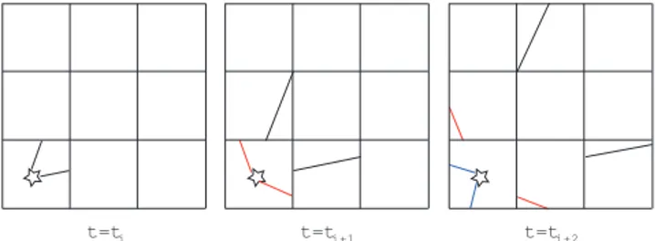
To minimise the amount of communication phases per time step, we follow a different approach by truncating the recursive solution of eq. 1 at the boundaries of the domains. Instead of letting rays pass through multiple sub-domains in one time-step, rays are only processed until they reach the boundary of the enclosing sub-domain. At the border, they are then passed on to the neighbouring sub-domain. Once received, however, they will not be immedi-ately processed by the neighbour. Propagation of the ray is continued in to the next time step. The scheme is illustrated in Fig. 2. In this way, each sub-domain needs to
communi-t=ti t=ti+1 t=ti+2
Figure 2. Illustration of rays propagating through the dis-tributed computational domain at three time-steps ti, ti+1, and
ti+2. To simplify the illustration, a box domain decomposition
strategy is shown, where each square resembles one sub-domain. Further we assume that the source only emits two rays per time-step. The rays are propagated to the edges of each sub-domain during one time step. Then they are passed on to the neighbour-ing sub-domain to be processed in the next time step.
cate only once per time step with all its neighbours, resulting in a highly efficient scheme, assuming that the computa-tional load is well distributed.
Propagation is thus delayed and a ray needs at most
≈2(NCPU)1/ 3time steps to pass through the box (assuming
equipartition). The delay with which a ray is propagated through the box depends on the size of the time-step and the number of cores used. The larger the time-step is, the bigger the delay. The same applies for the number of cores. If the crossing time of a ray in this scheme is well below the physical crossing time, the instant propagation approx-imation is considered retained. However rays will have dif-fering propagation speeds from sub-domain to sub-domain. In the worst case scenario a ray only passes through one cell of a sub-domain. Therefore the minimal propagation speed is vprop, min≈0.56∆l/ ∆t, where ∆l is the size of one cell, ∆t
the duration of one time step, and the factor 0.56 is the me-dian distance of a randomly oriented ray passing through a cell of size unity as given in Ciardi et al. (2001). If the
prop-agation speed of a packet is vprop, min≫c, the propagation
can be considered instantaneous, as in the original CRASH2.
Even if this condition is not fulfilled and vprop, min< c, the
resulting ionisation front and its evolution can still be cor-rectly modelled (Gnedin & Abel 2001), if the light crossing time is smaller than the ionisation timescale, i.e. when the ionisation front propagates at velocities much smaller than the speed of light. However the possibility exists, that near to a source, the ionisation timescale is shorter than the crossing time, resulting in the ionisation front to propagate at speeds artificially larger than light (Abel et al. 1999). With the seg-mented propagation scheme it has thus to be assured that the simulation parameters are chosen in such a way that the light crossing time is always smaller than the ionisation time scale.
The adopted parallelisation scheme can only be effi-cient, if the communication bandwidth per time step is sat-urated. Each time two cores need to communicate, there is a fixed overhead needed for negotiating the communication. If the information that is transferred in one communication event is small, the fixed overhead will dominate the com-munication scheme. It is therefore important to make sure that enough information is transferred per communication event for the overhead not to dominate the communication scheme. The original CRASH2 scheme only allowed for the
c
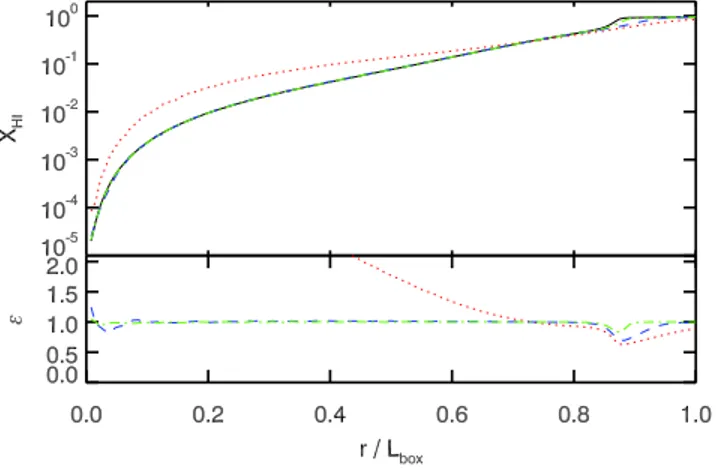
Figure 3.Test 0: Convergence study varying the number of pho-ton packets Np= 106,107,108,109used to simulate the evolution
of an H ii region. Shown are the spherically averaged neutral hy-drogen fraction profiles of the sphere as a function of radius at the end of the simulation. The dotted red line gives Np= 106, the
blue dashed line Np= 107, the green dash dotted line Np= 108,
and the black solid line Np = 109. The test used 8 CPUs. The
lower panel shows the relative deviation ǫ of the pCRASH2 run from the highest resolution run.
propagation of one photon packet per source and time-step. In order to avoid the problem described above, this restric-tion has been relaxed and each source emits multiple pho-ton packets per time step (Partl et al. 2010). Therefore in addition to the total number of photon packet produced per
source Np a new simulation parameter governing the total
number of time steps Ntis introduced. The number of
pack-ets emitted by a source in one time step is thus Np/ Nt.
As in CRASH2, the choice of the global time step should not exceed the smallest of the following characteristic time scales: ionisation time scale, recombination time scale, col-lisional ionisation time scale, and the cooling time scale. If this condition is not met, the integration of the ionisation network and the thermal evolution is sub-sampled.
3.3 Parallel pseudo-random number generators
Since CRASH2 relies heavily on a pseudo-random numbers generator, here we have to face the challenging issue of gen-erating pseudo-random numbers on multiple CPUs. Each CPU needs to use a different stream of random numbers with equal statistical properties. However this can be limited by the number of available optimal seeding numbers. A large collection of parallel pseudo random number generators is
available in the SPRNG library 4 (Mascagni & Srinivasan
2000). From the library we are using the Modified Lagged Fibonacci Generator, since it provides a huge number of
par-allel streams (in the default setting of SPRNG ≈ 239648), a
large period of ≈ 21310, and good quality random numbers.
On top each stream returns a distinct sequence of numbers and not just a subset of a larger sequence.
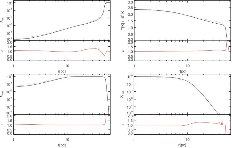
Figure 10.Test 3: Realistic H ii region extending in a hydrogen + helium medium. Compared are equilibrium results obtained with CRASH2 (black solid line) to ones obtained with pCRASH2 (red dotted line). The upper left panel gives the profile of neutral hydrogen fractions, lower left panel gives singly ionised helium fractions, and the lower right panel gives the double ionised helium fractions. The upper right panel gives the spherically averaged temperature profile as a function of radius.The small bottom panels show the relative deviation of the pCRASH2 run from the CRASH2 reference solution.
formation of H ii regions from multiple sources is followed in a static cosmological density field at redshift z = 9, including photo-heating. The initial temperature is set to T = 100 K. The positions of the 16 most massive halos are chosen to
host 105 K black-body radiating sources. Their luminosity
is set to be proportional to the corresponding halo mass and all sources are assumed to switch on at the same time. No periodic boundary conditions are used. The ionisation
fronts are evolved for ts = 4 × 10⁷ yr. Each source produces
Np= 1 × 10⁷ photon packets. pCRASH2 is run with Nt= 106
time steps on 16 CPUs.
A comparison between slices of the neutral hydrogen fraction and the temperatures obtained with pCRASH2 and
CRASH2 are given in Fig. 11 for t = 0.05 Myr and Fig. 12
for t = 0.2 Myr. For both time steps the pCRASH2 results produce qualitatively similar structures compared to CRASH2 in the neutral fraction and temperature fields. Slight dif-ferences however are present, mainly in the vicinity of the ionisation fronts, due to the differences in how recombina-tion is treated, as already discussed. In the lower panels of the same figures we show also the probability distribution functions for the hydrogen neutral fractions and the temper-atures. Here the differences are more evident. The neutral fractions obtained with pCRASH2 do not show strong devia-tions from the CRASH2 solution. In the distribution of tem-peratures however, pCRASH2 tends to heat up the initially
cold regions somewhat faster than CRASH2, as can be seen by the 20% drop in probability for the t = 0.05 Myr time step at low temperatures. This can be explained by the fact that the dominant component to the ionising radiation field in the outer parts of H ii regions is given by the radiation emitted in recombinations. The better resolution adopted in
pCRASH2for the diffuse field is then responsible for slightly
larger H ii regions. Since a larger volume is ionised and thus hot, the fraction of cold gas is smaller in the pCRASH2 run, than in the reference run. At higher temperatures however, the distribution functions match each other well. Only in the highest bin a discrepancy between the two code’s solutions can be noticed, but given that there are at most four cells contributing to that bin, this is consistent with Poissonian fluctuations.
4.3 Scaling properties
By studying the weak and strong scaling properties of a code, it is possible to assess how well a problem maps to a distributed computing environment and how much speed increase is to be expected from the parallelisation. Strong scaling describes the scalability by keeping the overall prob-lem size fixed. Weak scaling on the other hand refers to how the scalability behaves when only the problem size per core
c
F
ig u
Figure 15.Scaling achieved with Test 4 as a function of number of photon, optically thickness and number of CPUs.
cases. However, this can be easily understood as follows: The simulation time is set at five times the recombination time. Hence the same amount of recombinations per time step oc-cur (when normalised to the density of the gas) in both runs. Since recombination photons are produced when a certain fraction of the gas has recombined, the number of emitted recombination photons is similar in the two runs. Therefore the amount of CPU time spent in the diffuse component is similar and the scaling does not change.
4.3.3 Test 4
By studying the scaling properties of Test 4, we can in-fer how the code scales with increasing number of sources. Since Test 4 uses an output of a cosmological simulation, the sources are not distributed homogeneously in the do-main. Therefore large portions of the grid remain neutral as is seen in Fig. 12. This poses a challenge to our domain decomposition strategy and might deteriorate scalability.
First we study the scaling of the original Test 4, with
a sample of 108 photon packets emitted by each of the 16
sources. Then we increase the number of photons per source
to 109. Since large volumes remain neutral, we further study
an idealised case, where the whole box is kept highly ionised by initialising every cell to be 99% ionised. The results of these experiments are shown in Fig. 15. In the case of only
108 photon packets per source, good scaling can only be
reached up to 8 CPUs (i.e. a single node), as was the case with only one source. Communication over the network can-not be saturated with such a small number of photons and its overhead is larger than the time spent in computations. However by increasing the number of samples per time-step improves scaling. In the idealised optically thin case, perfect scaling is reached even up to 16 CPUs and starts to degrade for higher numbers of CPU. The discrepancy between the neutral and fully ionised case shows the influence of load imbalance due to the large volumes of remaining neutral gas.
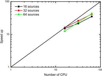
Since good scaling was found in the original Test 4, we now increase the number of sources. For this we dupli-cate the sources in Test 4, and mirror their position at an
Figure 16.Scaling achieved with Test 4 as a function of number of sources and number of CPUs for an ideal optically thin case.
Up to now we have only considered the case of a 1283
box. We now re-map the density field of Test 4 to 2563 and
5123grids. The resulting scaling properties for the ideal
op-tically thin case with 64 sources are presented in Fig. 17. The scaling properties are not dependent on the size of the grid, and weak scaling only exists as long as the number of cores does not exceed the number of sources.
We can thus conclude that our parallelisation strategy shows perfect weak scaling properties when increasing the numbers of sources (compare Fig. 16). Increasing the size of the grid does not affect scaling. However weak scaling in terms of the grid size only works as long as the number of CPUs does not exceed the number of sources (see Fig. 17 going from 64 to 128 CPUs).
From these tests, we can formulate an optimal choice for the simulation setup. We have seen that better scaling is achieved with large grids. Further linear scaling can be achieved in the optically thin case by using up to as may cores as there are sources. For the optically thick case how-ever, deterioration of the scaling properties needs to be taken into account.
4.4 Dependence of the solution on the number of
cores
Since each core has its own set of random numbers, the solu-tions of the same problem obtained with different numbers of cores will not be identical. They will vary according to the variance introduced by the Monte Carlo sampling. To illus-trate the effect, we revisit the results of Test 2 and study how the number of cores used to solve the problem affects the solution.
The results of this experiment are shown in Fig. 18, where we compare the different solutions obtained with var-ious numbers of CPUs. Solely by looking at the profiles, no obvious difference between the runs can be seen. Variations can only be seen in the relative differences of the various runs which are compared with the single CPU pCRASH2 run.
At t = 107yr the runs do not show any differences. In
Sec. 4.2.2 we have seen, that recombination radiation has not yet started to be important. This is exactly the reason why, at this stage of the simulation, no variance has devel-oped between the different runs. Since the source is always handled by the first core and the set of random number is always the same on this core no matter how many CPUs are used, the results are always identical. However as soon as the Monte Carlo sampling process start to occur on multiple nodes, the set of random numbers starts to deviate from the single CPU run and variance in the sampling is introduced.
At the end of the simulation at t = 5 × 10⁸ yr, large parts
of the H ii region are affected by the diffuse recombination field and variance between the different runs is expected. By looking at Fig. 18, the Monte Carlo variance for the neutral hydrogen fraction profile lies between 1% and 2%. The tem-perature profile is not as sensitive to variance as the neutral hydrogen fraction profile. For the temperature the variance lies at around 0.1%.
4.5 Thousand sources in a large cosmological
density field
Up to now we have discussed pCRASH2’s performance with controlled test cases. We now demonstrate pCRASH2’s abil-ity to handle large highly resolved cosmological densabil-ity fields embedding thousands of sources. We utilise the
z = 8.3 output of the MareNostrum High-z Universe
(Forero-Romero et al. 2010) which is a 50 Mpc h−1 SPH
simulation using 2×10243particles equally divided into dark
matter and gas particles. The gas density and internal
en-ergy are assigned to a 5123 grid using the SPH smoothing
kernel. A hydrogen mass fraction of 76% and a helium mass fraction of 24% are assumed.
The UV emitting sources are determined similarly to the procedure used in Test 4 of the comparison project (Iliev et al. 2006) by using the 1000 most massive haloes in the simulation. We evolve the radiation transport simulation
for 106 yr and follow the hydrogen and helium ionisation, as
well as photo-heating. Recombination emission is included.
Each source emits 108 photon packets in 107 time steps. In
total 1011 photon packets are evaluated, not counting
re-combination events. The simulation was run on a cluster using 16 nodes, with a total of 128 cores. The walltime for the run as reported by the queuing system was 143.5 hours; the serial version would have needed over two years to finish this simulation.
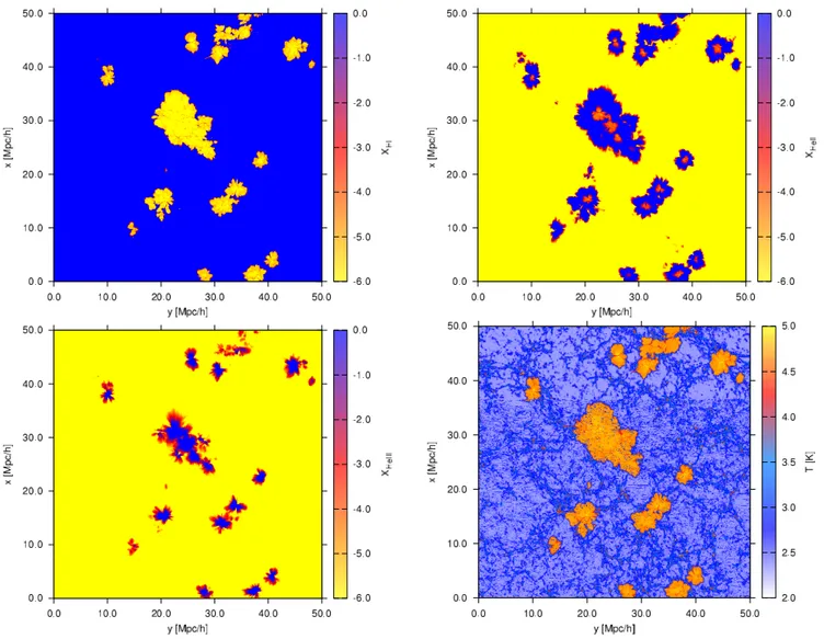
In Fig. 19 cuts through the resulting ionisation fraction
fields and the temperature field are shown at t = 106 yr.
It can be clearly seen that the H ii regions produced by the different sources already overlap each other. Further the ionised regions strongly deviate from spherical symmetry. This is caused by the fact that the ionisation fronts propa-gate faster in underdense regions than in dense filaments.
The distribution of He ii follows the distribution of ionised hydrogen, except in the centre of the ionisation regions, where helium becomes doubly ionised and holes start to emerge in the He ii maps. Photo-heating increases the temperature in the ionised regions to temperatures of around 30000 K.
These results are presented here as an example of highly interesting problems in cosmological studies which can be easily addressed with pCRASH2, but that would be impossible to handle with the serial version of the code CRASH2.
5 SUMMARY
We have developed and presented pCRASH2, a new paral-lel version of the CRASH2 radiative transfer scheme code, whose description can be found in Maselli et al. (2003), Maselli et al. (2009) and references therein. The paralleli-sation strategy was developed to map the CRASH2 algorithm to distributed memory machines, using the MPI library.
In order to obtain an evenly load balanced parallel al-gorithm, we statically estimate the computational load in each cell by calculating the expected ray number density as-suming an optically thin medium. The ray density in a cell is then inversely proportional to the distance to the source squared. Using the Peano-Hilbert space filling curve, the do-main is cut into sub-dodo-mains; the integrated ray number density in the box is determined and equally divided by the
c
Figure 19.Cut through a cosmological simulation at z = 8.3 with the neutral hydrogen fraction field (upper left panel), the singly ionised helium fraction (upper right panel), the doubly ionised helium fraction (lower left panel), and the temperature field (lower right panel) at time-step t = 1 × 10⁶ yr using 1000 sources.
in terms of clustering (i.e. that all points on the curve are spatially near to each other) is the Peano-Hilbert curve. We will now sketch the fast Peano-Hilbert algorithm used by the domain decomposition algorithm for projecting cells on the grid which is a subset of the natural numbers including
zero N30 onto an array in N10. A detailed description of its
implementation is found in Chenyang et al. (2008).
Let HN
m, (m > 1, N > 2) describe an N -dimensional
Peano-Hilbert curve in its mth-generation. HN
m thus maps
NN0 to N10, where we call the mapped value in N10 a
Hilbert-key. A mth-generation Peano-Hilbert curve of N -dimension
is a curve that passes through a hypercube of 2m
×. . .×2m =
2m N in NN
0. For our purpose we only consider N 6 3.
Let the 1st-generation Peano-Hilbert curve be called a
N-dimensional Hilbert cell CN (see Fig. A1 for N = 2). In
binary digits, the coordinates of the C2[Hilbert-key] Hilbert
cell can be expressed as C2[0] = 00, C2[1] = 01, C2[2] =
11, and C2[3] = 10, where each binary digit represents one
coordinate XN in NN0 with the least significant bit at the
end, i.e. C2[i ] = X
2X1. For N = 3 the Hilbert cell becomes
C3[0] = 000, C3[1] = 001, C3[2] = 011, C3[3] = 010, C3[4] =
110, C3[5] = 111, C3[6] = 101, C3[7] = 100.
The basic idea in constructing an algorithm that maps
NN0 onto the mth-generation Peano-Hilbert curve is the
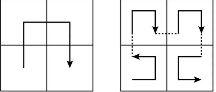
fol-lowing. Starting from the basic Hilbert cell, a set of coor-dinate transformations which we call Hilbert genes is ap-plied m-times to the Hilbert cell and the final Hilbert-key is obtained. An illustration of this method is shown in Fig. A1. Here the method of extending the 1st-generation 2-dimensional Peano-Hilbert curve to the 2nd-generation is shown. Analysing the properties of the Peano-Hilbert curve reveals that two types of coordinate transformations oper-ating on the Hilbert cell are needed for its construction. The exchange of coordinates and the reverse operation. The
ex-change operation X2↔X3 on 011 would result in 101. The
reverse operation denotes a bit-by-bit reverse (e.g. reverse
X1, X3 on 010 results in 111). Using these transformations
and the fact, that the mth-generation Hilbert-key can be extended or reduced to an (m + 1)- or (m − 1)th-generation Hilbert-key by bit-shifting the key by N bits up or down,
c
Figure A1.Left panel: The Hilbert cell C2 ≡ H2
1 for N = 2.
Right panel: Applying the N = 2 Hilbert genes on the Hilbert cell produces the 2nd-generation Peano-Hilbert curve.
the Hilbert-key can be constructed solely using binary op-erations.
For the N = 2 case illustrated in Fig. A1 the Hilbert
genes GN[Hilbert-key] are the following: G2[0] = exchange
X1and X2, G2[1] = no transformation, G2[2] = no
transfor-mation, and G2[3] = exchange X
1 and X2 plus reverse X1
and X2. Through repeated application of these
transforma-tions on the mth-generation curve, the (m + 1)th-generation can be found.
The Hilbert genes for N = 3 are: G3[0] = exchange X1
and X3, G3[1] = exchange X2 and X3, G3[2] = no
transfor-mation, G3[3] = exchange X1 and X3 plus reverse X1 and
X3, G3[4] = exchange X1 and X3, G3[5] = no
transforma-tion, G3[6] = exchange X2 and X3 plus reverse X2 and X3,
and G3[7] = exchange X
1 and X3 plus reverse X1 and X3.
ACKNOWLEDGMENTS
This work was carried out under the HPC-EUROPA++ project (project number: 211437), with the support of the European Community - Research Infrastructure Action of the FP7 Coordination and support action Programme (ap-plication 1218). A.P. is grateful for the hospitality received during the stay at CINECA, especially by R. Brunino and C. Gheller. We thank P. Dayal for carefully reading the manuscript. Further A.P. acknowledges support in parts by the German Ministry for Education and Research (BMBF) under grant FKZ 05 AC7BAA. Finally, we thank the anony-mous referee for important improvements to this work.
REFERENCES
Abel T., Norman M. L., Madau P., 1999, ApJ, 523, 66 Abel T., Wandelt B. D., 2002, MNRAS, 330, L53 Ahn K., Shapiro P. R., 2007, MNRAS, 375, 881
Alme H. J., Rodrigue G. H., Zimmerman G. B., 2001, The Journal of Supercomputing, 18, 5
Amdahl G. M., 1967, in AFIPS ’67 (Spring): Proceedings of the April 18-20, 1967, spring joint computer conference Validity of the single processor approach to achieving large scale computing capabilities. ACM, New York, NY, USA, pp 483–485
Baek S., Di Matteo P., Semelin B., Combes F., Revaz Y., 2009, A&A, 495, 389
Bianchi S., Ferrara A., Giovanardi C., 1996, ApJ, 465, 127
Chenyang L., Hong Z., Nengchao W., 2008, Computational Science and its Applications, International Conference, 0, 507
Ciardi B., Ferrara A., Marri S., Raimondo G., 2001, MN-RAS, 324, 381
Forero-Romero J. E., Yepes G., Gottl¨ober S., Knollmann
S. R., Khalatyan A., Cuesta A. J., Prada F., 2010, MN-RAS, 403, L31
Gnedin N. Y., Abel T., 2001, New Astronomy, 6, 437 Hasegawa K., Umemura M., 2010, ArXiv e-prints
Iliev I., Ciardi B., Alvarez M., Maselli A., Ferrara A., Gnedin N., Mellema G., Nakamoto T., Norman M., Ra-zoumov A., Rijkhorst E.-J., Ritzerveld J., Shapiro P., Susa H., Umemura M., Whalen D., 2006, Mon. Not. R. Astron. Soc., 371, 1057
Iliev I. T., Mellema G., Pen U., Merz H., Shapiro P. R., Alvarez M. A., 2006, MNRAS, 369, 1625
Iliev I. T., Whalen D., Mellema G., Ahn K., Baek S., Gnedin N. Y., Kravtsov A. V., Norman M., Raicevic M., Reynolds D. R., Sato D., Shapiro P. R., Semelin B., Smidt J., Susa H., Theuns T., Umemura M., 2009, MNRAS, 400, 1283
Jonsson P., 2006, MNRAS, 372, 2 Juvela M., 2005, A&A, 440, 531
Knollmann S. R., Knebe A., 2009, ApJS, 182, 608 Marakis J., Chamico J., Brenner G., Durst F., 2001,
Inter-national Journal of Numerical Methods for Heat & Fluid Flow, 11, 663
Mascagni M., Srinivasan A., 2000, ACM Trans. Math. Softw., 26, 436
Maselli A., Ciardi B., Kanekar A., 2009, MNRAS, 393, 171 Maselli A., Ferrara A., 2005, MNRAS, 364, 1429
Maselli A., Ferrara A., Ciardi B., 2003, MNRAS, 345, 379 McQuinn M., Lidz A., Zahn O., Dutta S., Hernquist L.,
Zaldarriaga M., 2007, MNRAS, 377, 1043
Mellema G., Iliev I. T., Alvarez M. A., Shapiro P. R., 2006, New Astronomy, 11, 374
Mihalas D., Weibel Mihalas B., 1984, Foundations of radi-ation hydrodynamics
Paardekooper J., Kruip C. J. H., Icke V., 2010, A&A, 515, A79+
Partl A. M., Dall’Aglio A., M¨uller V., Hensler G., 2010,
ArXiv e-prints, arxiv:1009.3424
Pawlik A. H., Schaye J., 2008, MNRAS, 389, 651 Petkova M., Springel V., 2009, MNRAS, 396, 1383 Razoumov A. O., Norman M. L., Abel T., Scott D., 2002,
ApJ, 572, 695
Ricotti M., Gnedin N. Y., Shull J. M., 2002, ApJ, 575, 49 Rijkhorst E.-J., Plewa T., Dubey A., Mellema G., 2006,
A&A, 452, 907
Rijkhorst E.-J., Plewa T., Dubey A., Mellema G., 2006, Astronomy & Astrophysics, 452, 907
Ritzerveld J., 2005, A&A, 439, L23
Ritzerveld J., Icke V., Rijkhorst E., 2003, ArXiv Astro-physics e-prints
Springel V., 2005, MNRAS, 364, 1105 Susa H., Umemura M., 2006, ApJ, 645, L93 Teyssier R., 2002, A&A, 385, 337
Trac H., Cen R., 2007, ApJ, 671, 1
Whalen D., Norman M. L., 2006, ApJS, 162, 281
c