3 Experimental Equipment and Techniques
3.1 Experimental Equipment
3.1.1 Vessel and Air Injection System
To model the aluminium furnace, water was used as fluid because it has a similar kinematic viscosity to the liquid aluminium. On the other hand, air has been accepted as the best way of modelling the chlorine gas (though the surface tension is different); also because a chlorine/nitrogen mixture is often used in the real industry. All the
experiments have been conducted in a rectangular-parallelepiped shaped (1/10 scale down of the real dimension of a typical aluminium treatment furnace), i.e. 650x252x190mm filled with distilled water to a height of 130mm, with a final working volume of ∼21 l. The gas was introduced in the system using a Plexiglas rigid pipe with a bore of
∼1mm, while the gas supplying system was a compressor connected to a rotameter to achieve the requested gas flow rate (Figure 3-1). The gas flow rate has also been scaled down to give two values maintaining equal the vvm (volume of gas per volume of liquid per minute) parameter, i.e. 0.1 and 1 l/min equivalent to 0.0048 and 0.048 vvm respectively.
3.1.2 Impeller Systems
Based on a work in The Department of Chemical Engineering of the University of Birmingham 12, three different impeller systems were investigated for this project. The main aim was to find the optimum configuration in terms of both good fluid motion and large spreading of gas. The following impellers were used:
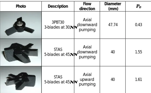
q 3PBT30, is a 3 pitch blades turbine, positioned with an angle of 30° in order to obtain a downward pumping flow. This impeller is the best of several studied in the paper mentioned before; q STAS DOWN, is a scale-down (1/10) of an impeller designed by
S.T.A.S. - UNIGEC 2002, it has 5 blades angled 45°, the thickness of the impeller is ∼10mm; and the diameter is 40mm;
q STAS UP, has the same dimensions and shape as the previous impeller but an opposite angle of the blades, which aims to generate an up-pumping flow.
Geometrical and further impeller details are collected in the Table 3-1 and Table 3-2. Details of the power numbers are discussed in section Errore. L'origine riferimento non è stata trovata..
Table 3-1 : Impeller geometries
Photo Description direction Flow Diameter (mm)
P
03PBT30 3-blades at 30° Axial downward pumping 47.74 0.43 STAS 5-blades at 45° Axial downward pumping 40 1.55 STAS 5-blades at 45° Axial upward pumping 40 1.61
Table 3-2: Impellers geometry details
[mm] 3PBT30 STAS Blade thickness 1.33 5.00 Blade height 9.53 10.40 Hub diameter 17.95 18.00 Hub height 9.94 10.40 Shaft diameter 10.00 10.00
3.2 Experimental Techniques
3.2.1 Power Measurement: Torque Measure
The power absorption of impellers is one of the most important factors that influence the mixing equipment design, e.g. it gives information about impeller efficiency and an idea about two-phase system. To measure the power draw a torque-measuring device, produced by Coesfeld, Mess-Technik GMBH, was used; in fact the torque exerted onto the shaft is proportional to the power, based on the law:
Where,
P
= Power draw [W]N
= Rotational speed [rps]M
= Shaft torque [Nm]The equipment, above mentioned, measures the shaft torque using inside strain gauge, which work on the principle that it changes its electrical resistance when a strain is applied to it. Furthermore the output of this device gives both the rotational speed, in rps, and the signal of the torque, in mV; these two signals were recorded on a chart recorder. There was also the possibility to connect directly the equipment to a computer, but this could result in signal averaging, so a direct digital acquisition on chart was preferred. After collecting all the data on an Excel worksheet, they were correlated, as mentioned above, to give the power draw and the power number against the rotational speed or Reynolds number.
NM
3.2.2 Mixing Time Method: Iodine Decolourisation
The mixing time technique for visual decolourisation of iodine/iodide solution with sodium thiosulphate as tracer has been largely used in the Chemical Engineering department in Birmingham13. The main characteristics of an ideal tracer which sodium thiosulphate exhibits are shown in Table 3-3. This decolourisation reaction is optimized in presence of a starch indicator to obtain a colour transaction from dark brown (until a low concentration of 2x10⁻⁵M) to completely colourless.
The main reaction is the reduction of iodine by sodium thiosulphate i.e.
I
2+
2S
2O
32-=
2I
-+
S
4O
62- ; this reaction cannot be used in practice, because the iodine is almost insoluble in water, so an iodine solution was prepared by adding potassium iodide to dissolve it (+
−=
−3 (aq.)
2
I
I
I
). Therefore, the original equation can be rewritten correctly as:O
S
3I
O
2S
I
2- - 4 62 -3 2 3+
=
+
−The concentration of both iodine and sodium thiosulphate solutions used were 2N, these were prepared as follows:
Iodine solution:
1.
dissolve 400g of iodate-free potassium iodide in 0.5 l distilledwater in a 1.0 l volumetric flask;
2.
add in 254g of iodine, shake in the cold until all the iodine has3.
allow to reach room temperature, and add distilled water untilthe final volume is 1.0 l. This solution should be stored in a dark place.
Sodium Thiosulphate
1.
put in a 1 l volumetric flask 496.4g of sodium thiosulphatepentahydrate crystals and dissolve in distilled water up to 1.0 l;
2.
to preserve this solution longer, 0.2g of sodium carbonate couldbe added.
Table 3-3 Ideal tracer characteristics
q No interaction with the main fluids;
q Cause a distinct and detectable response for data acquisition; q Short injection time compared to the final mixing time;
q No limitation in number of trials.
The experimental procedure consists in:
a. Add 4.5ml of starch indicator solution to the bulk fluid (distilled water) and allow to mix well.
b. Add 3ml of iodine solution to the bulk fluid. Allow 5mins mixing.
c. Add 3.6ml of sodium thiosulphate (20% excess on iodine) on the surface of the liquid. Simultaneously start stopwatch timer. d. Stop the stopwatch timer when the bulk is completely
e. Successive trials are repeated from step b.; though, before a new experimentation the excess of sodium thiosulphate has to be neutralized with iodine.
Decolourisation mixing time is defined as the time required to completely change colour from dark brown to colourless. Although this method gave a subjective mixing time (influenced by the flow and the observer) the final values obtained are helpful in comparing the subject mixing time of different apparatus. Therefore, this method gave valuable understanding into vessel zoning and/or compartmentalization and contemporaneous videos were recorded for every trial.
3.2.3 Fluid Flow Pattern: Particle Image Velocimetry 2D & 3D
For a full understanding of the fluid flow pattern a PIV system, from TSI Incorporated, was used. This equipment permits to measure punctual and instantaneous velocity over an extended region of the flow. TSI 2D-PIV systems measure velocity by determining particle displacement over time using a double-pulsed laser technique. A laser light sheet illuminates a plane in the flow, and the positions of particles in that plane are recorded using a digital camera. After a known fraction of a second (?T
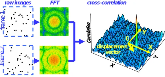
), another laser pulse illuminates thesame plane, creating a second particle image. Since particle images are in separate frames, every images have been subdivided in cells (16x16 pixels), which are analysed by the software with FFT method, after that a cross-correlation analysis gives the particle displacement for the entire flow region imaged. In Figure 3-2 is shown how the vectors have been calculated by the analysis of the cells.
Figure 3-2: PIV cross-correlation method
If the particles in the flow field move by an amount
? x ,
in thex-direction, and
? y
, in the y-direction, the velocities in thex
andy
directions are: T y v T x u=∆ /∆ and =∆ /∆ Eq. 3-2
Other properties, such as mean, turbulence and other higher order flow statistics can also be obtained using special software, Tecplot 8.0, provided with the PIV Equipment. Depending on the subject studied is possible to perform the PIV system changing some parameters as: the delay time between the two frames, number of pairs of images and the collection frequency. The delay time is dependent of the speed flow analysed, the maximum displacement of the image of the particles has to be less than 8 pixels, otherwise the FFT analysis is not able to properly correlate the image. For this work,
frame 1
frame
2
raw images
FFT
cross-correlation
displacement
vector
0
Y
X
15 pairs of image have been recorded for every trial, with a frequency of 15Hz, and afterwards all the velocity vector fields have been used to build a mean result.
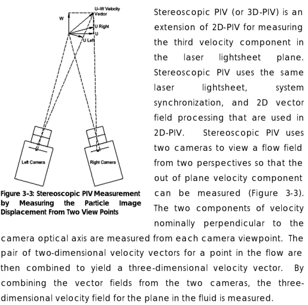
Stereoscopic PIV (or 3D-PIV) is an extension of 2D-PIV for measuring the third velocity component in the laser lightsheet plane. Stereoscopic PIV uses the same laser lightsheet, system synchronization, and 2D vector field processing that are used in 2D-PIV. Stereoscopic PIV uses two cameras to view a flow field from two perspectives so that the out of plane velocity component can be measured (Figure 3-3). The two components of velocity nominally perpendicular to the camera optical axis are measured from each camera viewpoint. The pair of two-dimensional velocity vectors for a point in the flow are then combined to yield a three-dimensional velocity vector. By combining the vector fields from the two cameras, the three-dimensional velocity field for the plane in the fluid is measured.
The following images show the TSI equipment used to collect the results for this thesis.
Figure 3-3: Stereoscopic PIV Measurement by Measuring the Particle Image Displacement From Two View Points
Figure 3-4: PIV Computer and synchronizer
3.2.4 Bubble Size: Video Measurement Technique
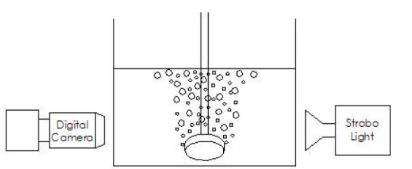
The bubble size is another important factor in aluminium cleaning process; in fac t the free surface available for the reaction between chlorine and impurities is directly correlated to the bubble dimension. To determine the bubble size distribution optical probe equipment was used, as described by Pacek et al.14. The data acquisition system
consisted of a high-resolution video camera combined with a low magnification stereomicroscope, a super VHS video recorder and a stroboscopic lighting system. All the images collected by the camera through the microscope were recorded on tape, and then downloaded on computer in order to analyze them with special software to give the number and the size of all bubbles.
For this work, the camera was positioned on one side of the vessel, while the stroboscopic light on the other, as shown in Figure 3-8. The area of interest was about 2cm above the impeller, and the system was focused in the middle of the vessel.