Development of a thermomechanical and metallurgical model in order to design a predictive control tool in line

(1)

Università Politecnica delle Marche

Scuola di Dottorato di Ricerca in Scienze dell’Ingegneria Corso di Dottorato in Ingegneria Industriale

---

Development of a thermomechanical and

metallurgical model in order to design a

predictive in line control system for

rolling process.

Ph.D. Dissertation of:

Alberto Nardini

Supervisor:

Prof. Mohamad El Mehtedi

Ph.D. Course coordinator: Prof. F. Mandorli

(2)

Abstract

Abstract

This project wants to build up a model which is able to predict mechanical properties achieved depending on parameters governing the inline thermal treatment developed by Siemens Metals Technologies between multiple rolling stages.

Such technologies consists in a specific treatment of quenching and tempering processes, like the Rail Head Hardening System that is actually the new evolutional technology to increase the performances in terms of safety and wear of the high speed train railways.

In order to guarantee a model which could be considered as more flexible as possible, the results want to be exploitable even in case of necessity to model other thermal processes.

The model will be developed in order to achieve the exact simulation for thermal treatment proposed by Siemens Metals Technologies, but it will be simply adjustable in order to allow predictions even in case of other thermal processes.

The approach which is going to be followed is the result of the compromise among the trial to develop a model on the state of the art, the in-field results offered by Siemens Metals Technologies and the experimental validation executable into the laboratories.

(3)

List of Contents

Chapter 1

1. Introduction

1.1 Preface

During the last 50 years, economic and technical demands have forced the steel industry to develop innovative processes to supply the transportation, energy and construction market with high strength, high toughness and cost-effective steels. While high strength can be easily achieved through the addition of solute strengthening or precipitation hardening elements, toughness cannot be significantly improved by alloy additions, but can be only achieved through the control of the final microstructure.

In particular in the present demanding SBQ and rail market, producers ask for high quality materials and high productivity at the lowest possible transformation costs. The plant suppliers’ challenge is to provide quality bars and rail producers with the most advanced and flexible technology available in order to match the market requirements and to move to an evolution of the product.

Since 1950, it was known that the refinement of microstructure improves both resistance to brittle fracture and strength of materials. Therefore research and development activities were focused on understanding how steels respond to hot processing and in-line cooling conditions and how that response can be altered by alloying, because the final microstructure after the phase transformation depends on the microstructure and composition of austenite just before the phase transformation and the evolution on the final metallurgical phases.

This has led to advances in both process and product metallurgy: the joint development of thermomechanical processes (TMP) and microalloyed steels (MA steels). While the aim of thermomechanical processing is the refinement of the austenitic grain size, the addition of microalloyed elements permits to better control the evolution of microstructure during processing.

In conventional hot rolling (CHR) both roughing and finishing pass are given to the material at the highest possible temperature in order to optimize productivity without taking into account the as-rolled mechanical properties and delegating the final balance between strength and toughness to subsequent heat treatments.

On the other hand TMPs can achieve a fine austenitic grain size either by lowering the temperature in roughing and finishing passes,

(7)

Chapter I - Introduction producing highly deformed austenite as in conventional controlled

rolling (CCR), or by controlling the evolution of microstructure, producing a fine fully recrystallized austenite as in recrystallization controlled rolling (RCR).

From an industrial point of view the main drawback of CCR is that it is not always applicable to rolling schedules because the power needed by mills to deform the materials raises as the temperature is lowered. The temperature involved in RCR, instead, can be sufficiently high to avoid excessive loads. RCR, therefore, can be a profitable way to balance processing needs with final product requirements.

However, in order to design a RCR rolling schedule it is necessary to have detailed models describing the recrystallization kinetics and evolution of the size of recrystallized and unrecrystallized austenite grains of steels during and between each deformation pass. Moreover, to be industrially effective, these models have to be coupled with Finite Element Modelling (FEM) that is widely used to calculate power, forces etc. needed by rolling mill and in tools design.

Microstructural models deeply changed in the last 25 years, evolving from empirical models to more physically based ones. However the growth of models complexity has been accompanied by a reduction of their applicability, since there is a lack of highly reliable data for the physical variables that are used in the calculations. Moreover physi-cally based models are not industrially used because, when coupled to FEM, the computational time become excessive.

Up to now, from and industrial point of view, only empirical models have proved to give satisfactory results, but these rely on a huge quantity of parameters that have to be calibrated by ad-hoc laboratory tests. Especially production of high quality bars and rails requires an accurate alloys design, rolling processes and thermal treatment strategies.

Therefore, the aim of this research is to develop an innovative in-line hardening flexible system applied for rails, named idRHa+®, able to enhance the mechanical properties desired and consequently increase service life up to three times compared to non-treated rails.

The work and the thesis have been organized as follows:

 Chapter 2 retraces the motivations of this research work birth,

starting from the geopolitical analysis of the industrial rail market, passing through the technical aspects and the production technologies in use, until it comes to its economic analysis.

 Chapter 3 is oriented to the description of the process

technology.

 Chapter 4 is devoted to a literary review about the

(8)

Chapter I - Introduction steel microstructural evolution, the mechanical properties and

their characterization methodologies used in this work.

 Chapter 5 is focused on the describing of the process control system developed.

 Chapter 6 presents the results obtained by the system through a

pilot plant.

 In the end, Chapter 7 provides the general conclusions of this research activity.

(9)

Chapter II – Business Analysis

Chapter 2

2. Business Analysis

2.1 Introduction

Transport is crucial for economic growth and poverty reduction. Almost nothing can be produced or consumed unless people, raw materials, commodities, fuel, and finished products can be moved to and from different locations. In many countries, railways are an important part of the transport network. With growing environmental concerns, and increasing congestion from personal vehicles, today many governments and organizations, see railways as a critical element of greener transportation and development.

Railways have a huge potential to contribute to developing country green growth agendas. There are several reasons for this:

 Railways are clean: Within the transport sector, rail accounts for 2% of CO2 emissions and rail is 3 to 10 times less GHG(greenhouse gas) intensive than other modes of transport.  Railways are efficient: In some market segments (e.g. bulk freight

over 800km, or passengers for up to four-hour trips) railways are the most efficient mode of transportation.

 Railways integrate easily with other modes of transport: Many cities have integrated public transport ticketing systems; rail stations are hubs for interchange with other modes - bus, taxi, car, cycle, and pedestrian; new advances in containers allow for more integrated freight transport with shipping and air transport.  Railways continue to innovate: Today’s electric rail transport is

free of direct local air pollution while innovative thinking in public-private partnerships is transforming many railways into modern, efficient, and revenue-generating enterprises.

 Railways take less space: Railway infrastructure occupies 2-3 times less land per passenger or freight unit than other modes of transport.

 Railways are safe: Although railways are not free of accidents, disproportionately more people die on world roads every year.

(10)

2.2 Rail Market

The production of rails in the world has reached a stable volume over 12 million tons/p.a., sustained by demographic, economic/political and technological drivers. The production plants overall capacity is quickly expected to approach the 15 million tons/p.a. and there are strong indications for a further push of growth towards 20 million/p.a. tons by the next decade. A network density close or higher than 0,05 km/km² is currently installed only in some limited areas of the world (fig.2.1), but represents a possible medium-term target for many other areas in most of the continents.

Figure 2.1 Rail Network density

Beside such network extension, there is then an arising tendency for the installation of higher quality tracks, mainly linked to the developments of high-speed or/and heavy-haul transport lines.

As known, the technical and the quality requirements of the rails are indicated in the relevant country or clusters Standards; the quick impulse of development of the rail technical qualities and performances, has therefore determined a parallel need of updating for many Standards. A clear example of this trend of updating of the International Standards, are the new European EN 13674-1:2011-04, the American ASTM A1-2010, the Russian GOST 51685-2011 (part of overall Technical Specification TU 0921 231 01124323-2007), the Indian IRS T12-2009 and the Chinese TB/T 2344-2012.

It can be noted that all Standards of the countries where the rails production poles are (figure 2.2) have been updated during the last 3-4 years, a clear indication of the dynamism of the strong technological evolution. In some cases (i.e. GOST ДT350-HH rail grade for extreme low-temperature applications), the Standards specify demanding features

(11)

Chapter II – Business Analysis even higher than those industrially obtainable with the current

production technologies and requiring processes still in consolidation or even in study.

Figure 2.2 Rail production map and network worldwide

Figure 2.3 represents graphically some typical rail technical requirements: the green bubbles are for standard not-alloyed/ not treated low strength pearlitic rails (about 80÷85% of the overall market) and the yellow bubbles for hard rails (10÷15% of the market, trend to increase), both alloyed and thermal treated. The red bubbles are instead relevant to some new-generation of rail grades which are currently in a study or prototyping phase.

Figure 2.3 Rail steels (present and future market) Elongation % U lti m a te T e n s il e Str e n g th (M p a ) 8% 13% 17% 22% 7 0 0 9 0 0 11 0 0 1 3 0 0 1 5 0 0 R320Cr R260, R260Mn I GEN II GEN High Strength pearlitic steels Low strength pearlitic steels R220 (A, B) R350LHT R370LHT R400UHT

III GEN TMCP pearlitic TMCP bainitic MARTENS Advanced High Strength Pearlitic, Bainitic, and Martensitic steels RAIL STEEL Typical production RAIL STEELS Allowable production RAIL STEELS critical/limited production

(12)

Chapter II – Business Analysis It has to be highlighted that the requirements are quite distant and

scattered in the graph, depending on the application and of the life-cycle, The figure 2.4 lists the major process technologies nowadays available to produce rails; the capability for a rail plant to produce efficiently a wide range of grades-sizes-lengths with quick automatic setup operations, self-adaptability of use governed by an intelligent process control system and at sustainable cost, is becoming more and more a must to be flexible and reactive in the world market scenario.

Figure 2.4 Major process production rails technologies available

This fast progression of the technical and economical requirements of the rails, challenges the capabilities of the Plant-makers to evolve their portfolio of solutions with incremental innovations..

The most modern solutions applicable in a rolling mill for rails can drive to a significant containment of the operational cost (i.e.-20÷30%) while producing products of superior quality (i.e. narrow size tolerances, consistency and uniformity of technical and metallurgical features) with higher added value; considering for instance the production of in-line thermal treated hardened rail, the price paid by market is, depending on countries, 8 to 20% higher than that of a standard untreated rail and with an estimated saving in production cost by at least 10%.

2.2.1 Problems and Improvements

Nowadays, the rapid rise in weight and speed of trains, has inevitably enhanced the rails wear rate, in terms of loss of material due to the abrasion between wheel and rail, and therefore an increasing of hardness has been required in order to reduce wear. With the increase of hardness

(13)

Chapter II – Business Analysis also the resistance to cracks damage and failure, therefore the

susceptibility to rolling contact fatigue (RCF), has been improved.

RCF is, by definition, damage of components that arises because of repeated loading associated with rolling contacts. A percentage of these cycles, under conditions of high friction and high contact stress, deforms the wheel and rail metal in the direction of the applied stress. The accumulating increments of deformation “ratchet” the surface layer. Although the effective strength of the material is increasing progressively because of strain hardening, it cannot strain indefinitely.

Figure 2.5(a) Kinematic Hardening, (b) Ratcheting in Rail Steels Associated with Contact Fatigue and (c) crack propagations.

Figure 1.6 shows an exemplification diagram of the necessity for a new apparatus able to improve rail steels mechanical properties.

Figure 1.6 Reasons for the search of new materials for rails

Conventional rail steels primarily contain nearly eutectoid pearlitic microstructure. Pearlite is an important feature of the microstructure

(14)

Chapter II – Business Analysis because it possesses good wear resistance, hence, making carbon an

essential alloying element in rail steels. However, it is not only the amount of pearlite that is important but also its morphology, which means the shape and the distance between the cementite lamellae. The finer the structure of pearlite, the higher is its strength whilst still retaining reasonable toughness. Therefore the development of pearlitic rail steels has been focused on the refinement of pearlite.

The strength of rail steels increases with a pearlite structure refinement whilst still retaining sufficient toughness. Therefore, the development of pearlitic rail steels has been focused on the refinement of pearlite. Two types of manufacturing processes have been applied to produce high strength pearlitic rail steels with fine lamellar spacing. One is to make the as-rolled high strength alloy steel rails whose hardenability is increased by the addition of alloying elements. The other one is to make a eutectoid carbon steel rail whose head is hardened by off-line or in-line heat treatment. The wear resistance of above-mentioned fine pearlitic rail steels has proved to be sufficient in practical use. However, with the extension of the rail life, rail surface damage by rolling contact fatigue came out as new challenge. In order to solve this new problem, the applicability of some bainitic steels was studied from literature results. The bainitic rail steels have high tensile strength and large elongation. Both fracture toughness and absorbed energy are much higher than those of head-hardened pearlitic rails. The wear resistance is nearly the same as in head-hardened pearlitic rails. Very long life span before shelling was also observed. The developed bainitic rails are expected to exhibit excellent performance in heavy haul railroads.

Pearlite comprises a mixture of relatively soft ferrite and a hard, brittle iron carbide called cementite, taking the form of roughly parallel plates. It achieves a good resistance to wear because of the hard carbide and some degree of toughness as a result of the ferrite's ability to flow in an elastic/plastic manner. Figure 2.7 (a) shows the microstructure of a pearlitic rail steel. The cementite is white and the ferrite is black. The interlamellar spacing is about 0.3 microns.

Correct choice of alloys and a correct cooling rate can produce a bainitic structure. This structure, like pearlite, normally contains ferrite and carbide, but in this case the ferrite is semi-coherent with the high temperature austenite phase from which it was formed. Alloying additions are made to prevent the formation of carbides, resulting in very fine interlath films of austenite which are retained between the ferrite plates. The structure is composed largely of low carbon carbide free bainite with some retained austenite. Figure 2.7 (b) shows the microstructure of a bainitic rail steel. The resulting bainitic rail steel has a high tensile strength of about 1400 MPa, and a large elongation. Both fracture toughness and absorbed energy by Charpy impact test are twice as high as those of head-hardened pearlitic rails. Wear resistance is nearly

(15)

Chapter II – Business Analysis the same than high strength pearlitic rails. Very long life span before

shelling was also observed, about twice as long as that of high strength pearlitic rails.

Figure 2.7 Microstructures of (a) pearlitic and (b) bainitic rail steels

At present, the situation for thermal treatments is different. There are only two means used to cool the rails: air or water. The water is typically used as liquid in a tank or sprayed with nozzles.

Air is typically compressed through nozzles. None of these arrangements allows producing all the rail microstructures with the same plant. In particular, a thermal treatment plant tuned for the treatment of pearlitic rails can hardly treat bainitic rails. Further present solution are not so flexible about possibility to treat the whole rail section or portions of the rail section in differentiated ways (head, web, foot).

The present invention overcomes the constraints previously mentioned by means of the flexibility of multi-means controlled cooling devices.

Figure 2.8 Accelerated control cooling unit-multi-means

The flexible system allows to obtain both high performance fine bainitic, pearlitic and hypereutectoid final microstructures by means of the same plant. Figure 2. show the different microstructure that can be created with the apparatus.

a

b

water forced air water+air accelerated control cooling unit hot rolled rails

(16)

Figure 2.9 Accelerated control cooling unit – different microstructures

heat treated pearlitic rails

hyper-eutectoidic pearlitic rails bainitic rails

hot rolled

rails accelerated control _{cooling unit}

UTS 1150÷1250 MPa YS 650÷700 MPa Hardness 320-370 HBN UTS up to 1400 MPa YS up to 870 MPa Hardness up to 500 HBN UTS 1300 MPa YS 750 MPa Hardness 410 HBN

(17)

Chapter III– Task description

Chapter 3

3. Task Description

3.1 Introduction

The final characteristics of a steel rail in terms of geometrical profiles and mechanical properties are obtained through a sequence of thermo-mechanical processes: a hot rail rolling process followed by a thermal treatment and a straightening step. The hot rolling process profiles the final product according to the designed geometrical shape and provides the pre-required metallurgical microstructure for the following treatment. In particular, this step allows the achievement of the fine microstructure which, through the following treatments, will guarantee the high level of requested mechanical properties

3.2 Concept design of the heat treatment system

At present, two main hot rolling processes, performed in two typologies of plant, reversible and continuous mills, are available (figure 3.1). The final properties of a rail produced by both of these hot rolling processes can be assumed as quite similar and comparable. In fact, bainitic, pearlitic and hypereutectoidic rails are commonly obtained at industrial level through both these kinds of plant.

Whereas the design of the hot rolling line is in some extent neutral to the quality of rails, the standard available solutions for the rail hardening treatment are not recognized so flexible and suitable to process efficiently all range of grades and selectively the whole rail section or portions of the rail section in differentiated ways (head, web, foot).

(18)

Figure 3.1 Best mechanical properties can be reached adopting strategies/apparatus put in the green blocks

Furthermore, in all the present industrial apparatus for thermal treatment of rails, most of the transformation of austenite occurs outside the cooling apparatus itself due to a number of technical and economic constraints, like space availability, process flow and productivity, cost of cooling media, outdated process controls. This means that the austenite transformation is not completely controlled, in particular when the austenite decomposition occurs, with an unrepressed increase of rail temperature due to the latent heat transformation. In this case, the temperature of austenite transformation is higher than the optimal one, with final mechanical characteristics lower than those potentially obtainable by finer and more homogeneous microstructures (fig. 3.2). This uncontrolled temperature profile is also critical for the bainitic rails, where the ideal path of transformation to obtain an homogeneous structure in the whole rail section (head, web and foot) is very narrow.

Top performance rail

(19)

Figure 3.2 Comparison between the correct/ideal cooling path and less controlled cooling process

Moreover, due to the real thermal profile of the rail along the length, a not or partially controlled thermal treatment unable to apply selective and variable cooling, can conduct to heterogeneous microstructures also along the length.

The design of idRHa+®, injector dual-phase Rail Hardening as the thermomechanical system is called, overcomes the limits previously mentioned by means of a more controlled thermal treatment, active on the rail until a significant amount of austenite is transformed (at least 50% on the rail surface and not less than 20% at the rail head core) This means that the austenite transformation temperature is maintained within a narrow ideal band thus avoiding any risk to produce secondary undesired structures: martensite for bainitic rails and martensite/bainite for pearlitic rails. The strict control of austenite transformation temperature is obtained by a dedicated flexible apparatus of suitable length equipped with multi-means controlled cooling devices, governed by an active process control system.

3.2.1 Process design of idRHa+

The process can be operated in-line or off-line in continuous or non-continuous rail process route. The essential feature of the in line heat treating process is the ability to transform the high temperature austenitic structure that exists immediately following the hot rolling process to the

(20)

Chapter III– Task description desired room temperature structure without the normal intermediate

steps of cooling to room temperature and then reheating (resolutionizing) prior to accelerated cooling.

Figure 3.3 (a) illustrates a schematic continuous cooling transformation of rail steel. Air cooling of conventional (no hardened) rail steel corresponds to path 1. Cooling along path 2 will produce a much finer pearlite but below point (d) on path 2, bainite and then untempered martensite will be produced instead of pearlite. The bainite and untempered martensite are not preferred transformation products when formed with pearlite. Ideally, cooling along path 3 would be preferred because only a very fine pearlite would be produced. The dashed line on path 3 is nearly isothermal indicating that the pearlite will be of uniform interlamellar spacing as opposed to the varying spacing achieved between points (a) and (b) on path 1. The key issue will be to produce such an isothermal type of transformation in a bainitic region of the transformation diagram. Figure 3.3 (b) shows the intermitted quenching action good for obtains homogeneous pearlite or bainite structures.

Figure 3.3 (a) Schematic Representation of a Continuous Cooling Transformation diagram and (b) Conceptual Illustration of Bainite Compared to Pearlite Surface Cooling Paths

The intermittent quenching action is achieved with water, air or air+water sprays applied to the head, web, and base of the rail.

A system of heating from room temperature, in case of off-line process or a system of heating to equalize the rail temperature after hot rolling, in case of in-line process, is adopted (fig. 3.4).

(21)

Figure 3.4 Schematic plant lay-out for in-line process and bypass configuration for off-line system.

The heating is applied with a series of high-power induction modules, with split top and bottom coils fed with individually powered IGBT converters. Some peculiar design features of the induction modules are hereby described.

The flexible thermal treatment apparatus is composed by modules, whose number and relative position depend on plant productivity, rail length/sizes and grades to be produces. Each module is equipped with a set of interchangeable cooling devices (spraying nozzles with mist-atomizers or air-jet blades). The rail entry temperature is kept in the range of 750÷1000°C measured on the running surface. The cooling is adjustable in the range of 0.5÷40°C/s (figure 3.5) as function of desired microstructure and final mechanical characteristics. The rail temperature at the apparatus exit is in the range of 300÷ 650°C depending on the treated grade.

(22)

Figure 3.5 Cooling rate capabilities depending on microstructure and final mechanical properties desired.

Any module can be controlled and managed alone or coupled with one or more modules. The process strategy (e.g. heating rate, cooling rate, temperature profile) is pre-defined as a function of the final product properties. The process control system uses several embedded thermal, mechanical and metallurgical models: i.e. models for austenite decomposition with microstructure prediction, for precipitation behavior, for thermal evolution with transformation heat calculation, for mechanical properties prediction, for deformation behavior (see figures 3.6 a-b).

(23)

Figure 3.6 Process control system scheme about thermo-mechanical and microstructural model

By means of above models, the control system manages and predicts the process and the product parameters according to:

 rail grade chemical composition;

 rail grade mechanical characteristics (e.g. hardness, strength)  hot rolling mill setup and procedures

 expected rail temperature in defined profile points (head, web and foot) and along the length (head, center, tail)

 expected austenite decomposition rate and transformation temperature.

The pre-set cooling strategy is then fine-tuned taking into account the actual parameters, measured or predicted with integrative data during the rail process route.

The use of the most suitable cooling mean and its working parameters (e.g. pressure, flow rate) are determined for each module according to the optimized process strategy suggested by the process models. This guarantees the application of an ideal cooling path all along the rail length and through each position in the transverse rail section. Very strict characteristic variation can be obtained avoiding formation of zone with too high or too low hardness and avoiding any undesired microstructure. The basis of the process control scheme is shown in figures 3.7.

(24)

Figure 3.7 Process control system scheme for automation procedures

After the measurement of the rail temperatures in different peculiar positions, the process control system takes into account also the actual chemistry of the rail, the target microstructure and the target mechanical characteristic. The temperature measuring devices, pyrometers or thermoscan cameras, keep the temperature continuously monitored: this set of data is used by the process control system to impose the fine regulation to the automation system in terms of selective use of cooling modules, cooling media flux, running speed of the rail in order to correct dynamically any recognized thermal heterogeneity along the rail length and across the rail section. The embedded process models define the cooling strategies in terms of heat to be removed selectively from the profile and along the length of the rail. A specific temperature drop in function of time is proposed in order to transform the austenite at the exit of the flexible apparatus in a percentage not lower than 50% on rail surface and not lower than 20% at rail head core.

3.2.2 Mechanical design of idRHa+

The idRHa+ rail hardening system is composed by a group of integrated devices, each with a specific functional and technological purpose.

The system is fully modular so that it can be assembled in several configurations according to the process needs, to the required level of productivity and to the existing plant constraints.

TSET TL1 TH1 TH2 TL2 NO correction correction correction alarm alarm

BASIC PRINCIPLES ABOUT COOLING STRATEGY

(25)

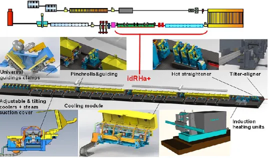
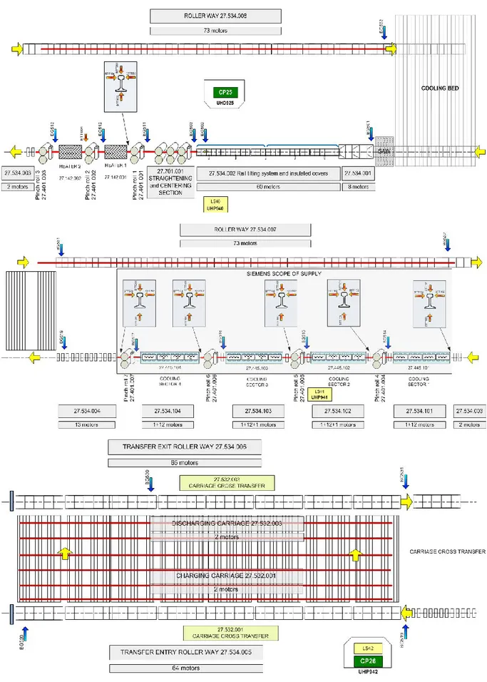
Chapter III– Task description The figure 3.8 shows a typical layout of an in-line idRHa+ system with its

functional units.

Figure 3.8 Typical layout of an in-line idRHa+ system with its functional units.

For in-line applications, after leaving the finishing stand or downstream the cooling bed, the rail is lifted in vertical position by a rail turning system whose center of rotation can be adjusted laterally to have any size of rail in the right upstream position to feed the idRHa+ line. The hot rail could be bent or have some waved parts along its length, especially in the first meters at its ends. It is therefore very useful to have a hot-straightening unit placed before the treatment line in order to recover a suitable straightness of the rail by soft plastic deformation applied by a group of vertically adjustable pinch-rolls.

A set of induction heating units, at least two, provide thermal energy to the rail to equalize the temperature along the length and adjust the suitable temperature distribution across the rail section; in order to have a sufficient buffer of integrative energy to recover the temperature gradients in the rail section and along its length, a typical installed power for an in-line idRHa+ treatment system is 30÷35 kW per ton of rolled rails, meaning that for a productivity of 150 tons/hours the installed power is about 5 MW. The setting of the induction units is pre-defined by a FEM modelling analysis and then dynamically tuned during operations depending on the detected evolution of the temperature profile. In fig. 3.9 an example of the results of the FEM analysis showing the temperature profile expected at the entry of the induction units and the corrected profile at the exit.

(26)

Figure 3.9 Thermal profile entry section HF(a) and exit section HF(b)

The design of the induction heaters is of extreme importance to grant a selective and efficient transfer of high power density to the rail in a short time and in a limited space. The induction heaters (coils) are split for the head and the foot of the rail and are fed by individual power converters designed with IGBT (insulated gate bipolar transistor) technology for maximum efficiency and control at optimized consumption (figure 3.10).

Figure 3.10 Inductor heaters with IGBT Technology

The induction heaters are adjustable on the vertical and on the horizontal axis to follow the possible out-of-straightness of the rail and to adapt to the various processed sizes and shapes of rails, including asymmetric rails. The rail is kept guided through the inductors by horizontal and vertical pinch-rolls while the risk of contact of the rail against the ceramic walls is prevented by means of a contour-follower device with rollers (figure 3.11).

(27)

Figure 3.11 Inductor heaters assembly

After being heated by the induction units, the rail enters in the cooling area, the core of the idRHa+ technology. As said before, the line is composed by several cooling modules assembled in sequence for a total length granting a sufficient time to have in the rail head most of the austenite (>50% on the surface, 20% in the core) transformed.

Each module is equipped with a set of cooling ramps acting selectively on a part of the rail in order to grant the proper heat transfer coefficient as necessary to reach the desired features; they have also the function to keep balanced the temperature gradients in the rail section to contain excessive deformations. The coolers can be atomizing-mist nozzles, adjustable at different mix of media, and air-jet blades; the proper combination of the coolers along the line and their full interchangeability grant an absolute flexibility of use to match any different process requirements. The position of the coolers is adjustable by means of a cam-system to maintain the proper distance from the rail necessary for an optimized cooling effect and to adapt to the different treated rail sizes, including asymmetric rails. The coolers are mounted on hydraulically tiltable ramps to facilitate the accessibility for the maintenance operations. The modules are sealed with covers and equipped with a suction system to evacuate the produced steam; also the covers are hydraulically openable to give access to the cooling module (fig. 3.12).

(28)

Each module is equipped with a set of swinging hydraulic pinch-rolls to keep the rail laterally clamped and guided while moving through the coolers; the particular design of this device makes it adaptable to any size and shape of rail (figures 3.13 a-b).

Figure 3.13 Swinging hydraulic pinch-rolls system (a), different shape configuration (b)

In between the modules, there are a number of horizontal pinch-rolls equipped with vertical idle rollers to keep the rail centered and guided all along its length without distortion.

3.2.3 Main technical features

Downstream the cooling bed, the rail shall be turned in vertical position by a rail turning system. A set of induction heating units of variable power depending on productivity and rail temperature profile provides thermal energy to the rail to equalize the temperature along the length and adjust the suitable temperature distribution across the rail section. At the entry of the induction units, there are some devices to align/center the rail and also to apply a soft hot-straightening to recover anomalous bending of the rail. The rail head could also be cut before entering the induction units to remove abnormally bent part. A set of guiding pinch-rolls ensures a constant speed under the cooling section. After the heating phase the rail enters the cooling line, where it is cooled down following a dedicated cooling strategy in order to achieve the proper microstructure. The rails is then transferred by a transfer machine to cooling table entry way and then straightened.

(29)

(30)

3.2.3.1 Straightener

The straightening and centering system is used to align/center the rail before sending it into the induction heaters. It applies soft hot-straightening to recover anomalous bending of the rail.

It is equipped with a hydraulic system that is used for opening and closing the top rolls, lifting and lowering the bottom rolls, opening and closing the vertical rolls, and 3 sets of AC motors controlled by single drives for the rollers rotation motion.

Another set of 3 AC motors, connected to a screw jack, is used to adjust the closing distance of the top rollers that is controlled by absolute encoders. By adjusting different heights of the three rollers, it is possible to straighten the rail when it is passing.

Figure 3.15 Straightener concept

The automatic cycle is enabled only when the actual values for the position adjustments all correspond to the set-point values.

As soon as the rail is ready after tilting, the rollers start running at the requested speed and the entry roller way delivers the rail to the straightening machine. The downstream process will then take control for the speed reference and decelerate or accelerate according to the hardening process.

3.2.3.2 Induction Heater

The Induction Rail Heater is located on the entry of the Flexible Rail Hardening System to raise the rails temperature to the target value before the cooling process.

To maximize the efficiency of the induction heating, the coils must be as close as possible to the rail, therefore the rail must necessarily has a suitable controlled profile in its length; the rail straightness can be

(31)

Chapter III– Task description detected by mechanical (contact rollers) systems to allow the induction

units to adjust their position (in vertical and in horizontal planes) to follow the contour of the incoming rail. Reasonable deviation can be tolerated otherwise the induction units are opened to avoid damages by contact with the protecting layer of the coils.

The heater is composed of two inductors, one on the top a another on the bottom of the rail pass line. The top inductor closing gap adjustment is done by an AC motor, controlled by an absolute encoder, that drives a jack screw. The top inductor can be lifted and lowered by means of a proportional hydraulic valve, in order to control the lowering phase with acceleration and deceleration in time. The top inductor’s actual position is monitored by two end position sensors, to detect the UP or DOWN position. The bottom inductor can be lifted and lowered by means of a double solenoid hydraulic valve. The top inductor’s actual position is monitored by two end position sensors, to detect the UP or DOWN position.

The automatic cycle is enabled only when the actual values for the top inductor height adjustment corresponds to the set-point value.

The induction heater waits for the rail’s head with the top inductor in the UP position and the bottom inductor in the DOWN position. The rail enters the heater area pushed by the upstream pinch roll, that also has the function to center it with the vertical rollers. After the heater there is the downstream pinch roll that will receive the rail head, and close on the rail. As soon as the rail is pinched with the two pinch rolls, the inductors “close” on the rail by lifting the bottom inductor and lowering the top inductor. The actual temperature of the rail is measured on the entry side of the Heater, and this value is sent to the Induction Heater Automation System, as well as the actual Rail speed.

Heater performance:

 Temperature variation along the rail length = ±20 °C

 Rail top target temperature after heating > 850°C (reheating of 100°C)  Rail foot target temperature after heating > 800°C (reheating of

100°C)

Temperatures are detected by the in-line pyrometers installed ahead of the first induction unit and after the second induction unit.

The measured temperatures will be averaged on a period of 3 seconds. The stress for the converter is calculated according to the following equation:

(32)

(3.1) Where:

K1 Proportional factor for all temperatures K2 Proportional factor for low temperatures

T0 Theoretical temperature where the reference stress for the converter is 0 - affects mostly high Temperatures

Tin Inlet Temperature of the head of the rail Tref Reference temperature at end of heater Tref0 Reference temperature for calculations M Mass of rail

m0 Reference mass of rail for calculation ( 60 kg/m ) V Rail Speed

v0 Reference rail speed ( 1000 mm/s) Ucorr Stress bias

Yui Upper inductor relative position to rail head

3.2.3.3 Temperature measurement

The temperature of the rail is measured in 4 points on the entrance of the cooling sector.

One pyrometer placed on top of the rail measures the top temperature, another two measure the side temperatures and a fourth one the foot temperature.

Figure 3.16 Pyrometers positions

3.2.3.4 Water & Air pressure control

The cooling process control is common for each pair of 2 air/mist modules. It is divided into four individual systems for the TOP, LEFT SIDE, RIGHT SIDE and FOOT cooling regulation for water, and three for AIR ( the left and right air control are a common system).

(33)

Chapter III– Task description pressure control. The three systems are separate for the TOP, SIDE and

FOOT part of the rail.

Each pair of modules have in common:

 A set of 4 proportional controlled water pressure regulation valves;  A set of 4 water pressure transducers;

 4 water draining valves for fine control of flow for low set points;  A set of 3 proportional controlled air pressure regulation valves;  A set of 3 air pressure transducers

In the case of only air module is used for cooling, every module use independent air pressure control valves and a feedback transducers.

(34)

Chapter IV– Literature review

Chapter 4

4. Literature review

4.1 Metallurgical model

Modeling and simulation of microstructure evolution is one of the most important ways to improve the quality of the final product. In order to optimize thermomechanical parameters for achieving the desired mechanical properties of the product, understanding and modeling microstructure evolution is a key issue for designers of metal forming processes (hot rolling, forging, and extrusion).

4.1.1 Transformation kinetics

A variety of phase transformations are important in the processing of materials and usually they involve some alteration of the microstructure. It is possible to identify three different kind of transformations:

1. Simple diffusion-dependent transformations and recrystallization, in which there is no change in either the number or composition of the phases present. These include solidification of a pure metal, allotropic transformations and recrystallization and grain growth; 2. Diffusion-dependent transformation governed by the presence of

some alteration in phase compositions and often in the number of phases present;

3. Diffusion less transformation, wherein a metastable phase is produced.

Due to the fact that in present work I will deal with transformation which involves only solid phases, the present section is going to be devoted to solid- state transformations. As Johnson and Mehl originally observed, phase transformations are usually the result of simultaneous process of nucleation and growth. Transformation progress is usually ascertained by either microscopic examination or measurement of some physical properties (such as electrical conductivity) whose magnitude is distinctive of the new phase. As it will be following proposed, data are usually plotted as the fraction of transformed material versus time as reported in fig. 4.1. Nucleation and growth stage are reported.

(35)

Figure 4.1 Fraction reacted versus the logarithm of time typical of many solid-state transformations in which temperature is held constant

4.1.2 Isothermal transformation kinetics

For an isothermal diffusional or reconstructive transformation i.e. for which T (t) = constant, the Johnson-Mehl-Avrami-Kolgomorov or “JMAK” equation is often used for the analysis of the experimental kinetic data:

f (t, T ) = 1 – exp [−k(T )tn_] _(4.1)

where f (t, T ) is the fraction transformed and t is the transformation time and n is the exponent, k is the reaction rate constant. It is given by:

k(T ) = k0 ·𝑒−

𝑄

𝑅𝑇 (2.2)

where Q is the activation energy for the transformation. The JMAK equation can be derived assuming constant nucleation and growth rates. The sigmoidal shape is a consequence of the small number of nuclei available for short times, the growth of many nuclei at intermediate times and impingement at longer times. The JMAK equation may be generalized to include an incubation time:

X(t, T ) = 1 – exp [−k(T )(t − τinc)n] (4.3)

The factors that influence f(t,T) are:

• the nucleation rate, which is function of the undercooling;

• the growth rate, which is temperature dependent in diffusion controlled transformations;

• the number of nucleation sites;

(36)

The rate of transformation is given by:

𝑑𝑋(𝑡,𝑇) 𝑑𝑡

= 𝑛𝑘𝑡

𝑛−1

_{(1 − 𝑋) = 𝑛𝑘(1 − 𝑋) [−}

ln⁡(1−𝑋) 𝑘

]

𝑛−1 𝑛 (4.4) In the isothermal case, the JMAK equation has a typical sigmoidal or S-shaped time dependence as the one reported in fig.4.1. The JMAK equation can be derived theoretically and the k and n value can be shown

to have a clear physical meaning. It is assumed that nucleation starts at t

= τ and the nuclei are spherical. Assuming the radius r of the phase

product has a linear rate of increase, i.e. its growth rate G is described by

G = 𝑑𝑟 𝑑𝑡⁄ , the volume of a single sphere of product phase nucleated at

time τ is, at time t, given by: 4 3

𝜋𝑟

3

₌

4 3

𝜋 [

𝑑𝑟 𝑑𝑡

(𝑡 − ⁡𝜏)]

3

= ⁡

4 3

𝜋𝐺

3

_{(𝑡 − ⁡𝜏)}

3_(4.5)

If constant rate of nucleation N is assumed, equal to the number of nuclei

generated per time unit in a unit volume, the number of nuclei generated in a time interval dt results to be N·dt. Therefore, the volume of product

phase formed in a unit volume within a time interval dt is given by:

𝑁

4 3

𝜋𝐺

3

_{(𝑡 − ⁡𝜏)}

3

_𝑑𝑡

_(4.6)

Taking the “overlap or impingement error” into account, the actual total volume of untransformed phase volume is given by the ”extended volume fraction”: Vtot (1−f ), where Vtot is the total volume of transforming phase

and f is the fraction of phase, which has already transformed. This

connection recognizes that a nucleus can only grow into a given volume of the untransformed material. The increase df in transformed fraction within a time interval dt is given by:

𝑑𝑓 =

1 𝑉𝑡𝑜𝑡

(1 − 𝑓)𝑁𝐺

3 4 3

𝜋(𝑡 − ⁡𝜏)

3

_𝑑𝑡

_(4.7) and hence: 𝑑𝑓 1−𝑓

=

4 3

𝑁𝐺

3

_{𝜋(𝑡 − ⁡𝜏)}

3

_𝑑𝑡

_(4.8)

This equation can be integrated to yield:

∫

_1−𝑓𝑑𝑓

= 𝑁

4 3

𝜋𝐺

3 𝑓 0

∫ (𝑡 − ⁡𝜏)

3

𝑑𝑡

𝑡 0

= ⁡

𝜋 3

𝑁𝐺

3

_{(𝑡 − ⁡𝜏)}

4_(4.9) Rearranging: f = 1 − exp(− N 𝜋 3G 3₍_{t − τ )}4₎ _(4.10)

(37)

Figure 4.2 The transformation-geometry dependent n values at constant nucleation rate N and growth rate G for spherical, plate and needle type growth of new phase.

When the nucleation rate goes to 0, only pre-existing nuclei grow and no new nuclei are generated during the transformation: this leads to a reduction of the n-value

This equation has the same general form as the JMAK equation. This deviation can be modified to show that the coefficient n is related to

particular types of transformation growth geometries as depicted in fig.4.2. The coefficients k and n can be calculated based on theoretical

transformation models. Both can be also determined experimentally by means of measured isothermal transformation kinetics using dilatometric data. Constant k depends on both the nucleation rate and the growth rate.

It is therefore very sensitive to the temperature. The activation energy Q,

is determined experimentally as follows. As the parameter k is given by eq.4.2, for two isothermal transformation measurements at T1 and T2 it is possible to write:

ln(𝑘

1

) = ln(𝑘

0

) −

𝑄

𝑅𝑇

₁

ln(𝑘

₂

) = ln(𝑘

₀

) −

𝑄

𝑅𝑇

₂

and subtracting each term:

ln(𝑘

1

) − ⁡ln(𝑘

2

) = −

𝑄 𝑅𝑇1

+

𝑄 𝑅𝑇2

→ 𝑙𝑛 (

𝑘1 𝑘2

) = ⁡

𝑄 𝑅

(

1 𝑇2

−

1 𝑇1

) (4.11)

Rearranging: 𝑄 = ⁡𝑅𝑙𝑛( 𝑘1 𝑘2) (1 𝑇2− 1 𝑇1) (4.12)

(38)

Figure 4.3 Schematic showing the method to determine k and n in the JMAK equation

4.1.3 Nucleation kinetics

Some important transformations that occur in steels, e.g. the formation of ferrite and perlite, are of “nucleation and growth” type, and the nucleation stage plays an essential role in the initial stages of the transformation. The nucleation of ferrite in austenite in pure Fe can be very fast. It is usually heterogeneous, which implies that the a−Fe nuclei are formed on low energy sites, usually grain boundaries or inclusions in the parent g–Fe phase. The rate of nucleation, I, i.e. the number of a–Fe nuclei that form per unit of volume and per unit of time in g–Fe, is described by the following equation:

I = Zn

_{𝑡𝑜𝑡𝑎𝑙}

𝑒

−∆𝐺∗𝑘𝑇

𝜔𝑒

− 𝑄 𝑘𝑇

(1 − 𝑒

𝑡 𝜏

)

(4.13) where:

• Z is the Zeldovitch factor, which takes into account the fact that only

a fraction of critical-sized embryos become nuclei.

• 𝑛∗₌

_n

𝑡𝑜𝑡𝑎𝑙

𝑒

−

∆𝐺∗

𝑘𝑇⁡is the number of a−Fe nuclei that have reached the critical size, assuming the total number of potential nucleation sites in g–Fe is given by ntotal.

This factor depends of the free energy variation

∆𝐺

∗_{associated with the}

formation of a heterogeneous critical nucleus of diameter r. This

situation is illustrated in fig.4.4, where it is shown a lens-shaped a−Fe nucleus with radius r on a grain boundary in g–Fe, which has surmounted the free energy barrier

∆𝐺

∗_{. A shape factor is used in order to take into}

account the geometry of the nucleus. In this case, it is equal to (2+cos 𝜃)(1−cos 𝜃)2

(39)

 𝛽 = ⁡𝜔𝑒−−_𝑘𝑇𝑄_{is the rate at which Fe atoms jump from the}

γ to the α phase. ω is the jump frequency to a suitable position in the nucleus.  𝑒−𝜏

𝑡, is a factor which takes into account the fact that an incubation time tau may pass before the nucleation starts. Schematic

representation is reported in fig.4.4. At lower temperatures the nucleation process is fully-diffusion controlled. The activation energy for diffusion entering into the calculation for the nucleation rate is not necessarily the activation energy for bulk diffusion. Grain boundary diffusion may have a much lower activation barrier. The TTT diagram of diffusional transformation transformations will usually have a “nose” or ”C” shape which is indicative of the fact that the rate of transformation is highest at an intermediate undercooling below the equilibrium transformation temperature. At temperatures close to the equilibrium transformation temperature the driving force for transformation is small and both nucleation and growth rates are low. At greater undercooling the transformation is again delayed due to the slow diffusion rates. Heating transformations, such as austenite formation from ferrite, exhibit a monotonic increase in kinetics with temperature because there is no ”trade-off” between driving force and diffusivity in heating transformations. Transformations in steel are complicated due to the fact that these are multicomponent systems requiring diffusion of different species. In general, the nucleation rate and the growth rate are functions of temperature as depicted in fig.4.5.

Figure 4.4 Scheme of the fundamental aspects that play a role during the nucleation process in solid state transformations in ferrous alloys. Nucleation of ferrite at austenite grain boundaries. Calculation of the critical free energy and critical size for nuclei. Determination of nucleation rate.

(40)

4.1.4 Empirical Methods

Simple empirical methods have been proposed to describe the transformation kinetics for steels based on parameters determined using non-linear least squares regression analysis of experimental data from a large number of steels. The temperature dependence of k, the reaction rate constant, is described by means of a modified Gaussian function:

𝑘⁡ = 𝑃1⁡𝑒𝑥𝑝 [− ( 𝑇−𝑃2

𝑃3 ) 𝑃4

]

(4.14)

Figure 4.5 Schematic of the temperature dependence of the nucleation rate N and the growth rate G, and the overall rate of transformation

TTT curves can easily be plotted if the Pi parameters are known. Pi

parameters have the following meaning:

• P1: the maximum value of k;

• P2: the temperature of the nose;

• P3: the width of the k function;

• P4: a parameter related to the sharpness of the k function;

• Ae3: temperature under which the existence of the ferrite becomes

thermodynamically possible. It can be simply evaluated such as:

Ae3 = 911−29%Mn−10%Cr+70%Si−(418−32%Mn+86%Si+1%Cr)·%C+232%C2

(41)

Chapter IV– Literature review Considering the austenite grain size dg in µm, the Pi parameters can be

evaluated as: • For ferrite: 𝑃1= 2 𝑑𝛾(%𝐶+%𝑀𝑛 6) 𝑃2= 𝐴𝑒3− 210 − ⁡170% 𝑃3= 67 𝑃4= 1.9 𝑛 = 1.5 (4.15) • For pearlite: 𝑃1= 213 𝑑𝛾 𝑃2= 𝐴𝑒1− 60 + 400 𝑑𝛾 − 470%𝐶 𝑃3= 47 𝑃4= 2.2 𝑛 = 1 (4.16)

For a hypo-eutectoid steel, there is an additional complication in the sense that pro-eutectoid ferrite can form.

4.1.5 Martensite transformation kinetics

The γ → α’ martensitic transformation in ferrous alloys is most often athermal, i.e. the fraction transformed is controlled by temperature changes rather than being time dependent. In TTT diagrams the extent of martensitic transformation is therefore represented as a series of parallel lines representing the transformed austenite fraction. The transformation kinetics can be described by an empirical time independent equation such as:

fα’ = 1 – exp (−a (M_s − T )n) (4.17) where fα’ is the fraction of austenite that has transformed to martensite,

Ms is the martensite start temperature and T is the temperature to which

the steel is quenched. According to Koinstinen and Marburger, the coefficients α and n are 0.011 and 1 respectively. It is necessary to underline that this is not the unique formula proposed to described

(42)

martensitic formation. Further equations, even of different shape (linear or exponential) exist. There are several formulas available in literature in order to determine the Ms temperature depending on chemical composition. According to:

Ms = 521 − 353%C − 26%M o − 22%Si − 24%M n − 17%Ni − 8%Cu + 18%Cr

(4.18)

4.1.6 Consideration on the use of JMAK equation

When JMAK equation is adopted, it is very important to take into account which hypothesis are assumed. In particular it is necessary to remark, as Humphreys noted that, the hypothesis at the basis of JMAK model are:

• random nucleation sites dispersed in the parent phase;

• the growth rate of the new phase is constant and not dependent on the extend of transformation;

• growth occurs at the same rate in all directions.

Depending if the nucleation rate will be constant or not during the whole transformation, the coefficient n can assume different values:

• n = 4: if the nucleation rate during the whole transformation is

constant;

• n = 3: id the nucleation occurs only at the beginning of the

transformation.

(43)

Chapter IV– Literature review Humphreys noted that is very unusual to find experimental data with

very good agreement with JMAK model. The Avrami exponent n is

measured on the ln(ln(1/(1 − X))) against ln(t) plot (the so called Avrami

plot) where it is represented by the slope of a straight line as reported in fig.4.6. However, it is frequent to find out some deviations from the linearity that indicate some non-modelled slowdown.

Figure 4.7 Example of inhomogeneities in the distribution of the stored energy

In real materials, the nucleation occurs in preferential sites and there are evidences that the growth rate of new grains is not a constant in the volume of the sample and during the recrystallization. Another justification for the typical trend of experimental Avrami plot is based on a not homogeneous distribution of the stored energy and can be used both for high and low stacking fault materials. As reported in fig.4.7, there are some regions (dark shaded) with high energy stored, resulting for example from local straining, dispersed into a matrix with lower energy values. New grains will nucleate inside or close to these regions and their growth will be initially fast but will decrease when regions with high energy stored are consumed. This ex- plains the non-random distribution of nucleation sites and the decreasing of growth rate with time. These complex phenomena cannot be fully predicted and because of this reason approximations achieved by JMAK model is univocally achieved by literature. Some authors proposed modifications, such as Khanna and Taylor arbitrarily did proposing a correction to the original JMAK equation. In particular, the correction proposed for the transformed fraction was:

X = 1 − exp(−Btk_{) →}_{X = 1 − exp(−(At)}k₎ _(4.19)

However Marangoni proved that Avrami equation should be used in its original form and the use of ”modified” version must be abandoned.

(44)

4.1.7 Non-isothermal transformation kinetics

In many practical situations, the temperature which governs a transformation of phase is not constant during the process. This is the case of many industrial processes. During heat treatments for steel, the transformation associated with austenite decomposition occur conditions of continuous cooling rather than isothermal conditions and the cooling rates may be different in different places as a result of the geometry of the part which has to treated. However, if the isothermal transformation kinetics are known, i.e. if the n-parameters and k-parameters of the JMAK

equation for isothermal transformation are available, the transformation kinetics during continuous cooling can be estimated. The cooling path T

(t) is therefore replaced by consecutive isothermal steps as represented in

fig.4.8. In the original version, the n-parameter is assumed to be

temperature independent while the k-parameter is assumed to be

temperature dependent.

Figure 4.8 Schematic show in the equivalence of a continuous cooling curve T(t) and a succession of small isothermal steps

The method is known as “Additivity rule” originally proposed by Scheil. The mathematics of the additivity principle are rather simple. Say one replaces the continuous T (t) by a succession of isothermal steps

lasting for a time ∆t at T1, T2..., Ti,. The first short isothermal hold at T1 will result in a ferrite fraction equal to f1:

𝑓1= 1 − 𝑒−𝑘1𝛿𝑡 𝑛

⁡ (4.20)

For the isothermal transformation at T2, a time 𝑡2∗ is defined: 𝑡2∗= √

𝑙𝑛(1−𝑓1) −𝑘2 𝑛