Insights into Mt. Etna volcano dynamics by seismic and infrasonic signals

Elettronica, Automatica e del

controllo di sistemi complessi

XIII CICLO

Placido Maria Montalto

INSIGHTS INTO MT. ETNA VOLCANO

DYNAMICS BY SEISMIC AND INFRASONIC

SIGNALS

Tutor: Prof. G. Nunnari Dr. D. Patanè Coordinatore: Prof. L. Fortuna INGV

SIGNALS

Elettronica, Automatica e del

controllo di sistemi complessi

XIII CICLO

Placido Maria Montalto

INSIGHTS INTO MT. ETNA VOLCANO

DYNAMICS BY SEISMIC AND INFRASONIC

SIGNALS

Tutor: Prof. G. Nunnari Dr. D. Patanè Coordinatore: Prof. L. Fortuna

Physical concepts are free creations of the

human mind, and are not, however it

may seem, uniquely determined

by the external world.

Preface

Active volcanoes are one of the most severe natural hazards in the world. Volcanoes are geologic manifestations of highly dynamic and complexly coupled physical and chemical processes in the interior of the Earth. They are complex dynamical systems that produce distinctive patterns. Volcanic eruptions are the culmination of a complex ensemble of processes that occur on a broad range of time scale, from tens or hundreds of years (e.g. magma rise and differentiation) to fractions of seconds (e.g. fragmentation). About 550 volcanoes have erupted in historical times. Reconstruction of the eruptive history of many volcanoes has shown that inactive periods of thousands of year are not uncommon (Scarpa and Gasparini, 1996). Historical data indicate that eruptions are almost always preceded and accompanied by “volcanic unrest” manifested by physical and/or geochemical changes in the state of the volcano (Tilling, 2008). Detection of precursory phenomena (e.g., seismic, geodetic, gravity signals, gas emission) is the main aim of volcano monitoring which provides parameters for early warning systems. Systematic collection and analysis of huge amount of data recorded on active volcanoes are performed for both research and monitoring purposes. The fact that strongly different precursory patterns can be observed for different eruptions at the same volcano means that there exists no universal sets of empirical parameters relating precursor to eruptions. However, data from volcano monitoring constitute the only scientific basis for short-term forecast of imminent eruption or changes in the volcano behavior. Most active volcanoes are routinely monitored

observing the pattern of the seismic activity and ground deformations. During the last years a key role in volcano monitoring is played by time series analysis methods and pattern recognition techniques, both in time and time-frequency domain, in order to detect and analyze different eruptive patterns. The aim of this thesis is the study of seismic and infrasonic signals generated by volcanoes using signal processing techniques and novel approaches based on nonlinear time series analysis and pattern recognition (PR) techniques. Chapter 1 is an overview on the state of the art of volcano monitoring. The description of methods applied to analyse different kinds of signal will be given in chapter 2. Chapter 3 deals with pattern recognition techniques largely applied on infrasonic signal treatment at Mt.Etna. In chapter 4 the methods used for seismo-volcano signal analysis will be described. In chapter 5, practical applications of the techniques depicted in chapters 2, 3, and 4 will be shown with the aim of investigating the infrasonic signals at Mt. Etna and their relationship with eruptive activity. While seismo-volcanic transients have been treated in literature using PR approaches (e.g. Del Pezzo et al., 2003; Scarpetta et al., 2005; Benitez et al., 2007), infrasonic signals characterization by PR techniques is brand new. Since infrasonic signals exhibit very suitable descriptive features, one of the most important topics that will be treated in this thesis, is the robust PR approach for infrasonic signals characterization and classification. In chapter 6 Mt. Etna volcano dynamics will be investigated from a seismo-volcanic point of view. In particular, in the second half of the chapter, a novel technique based on the multi station coherence will be used to highlight lava fountain precursor phenomena. Finally, in chapter 7 conclusions will be reported.

Acknowledgment

I would like to thank my scientific colleagues for their fundamental cooperation. In particular the following people deserve special mention: Dr. S. Alparone, Dr. Ferruccio Ferrari, Dr. G. Di Grazia and Dr. E. Privitera. A special acknowledgment goes to my colleagues and friends Dr. Andrea Cannata, Dr. Marco Aliotta and Dr. Ing. Michele Prestifilippo for their fundamental support in my scientific and personal growth. Many thanks to my tutors Prof. G. Nunnari and Dr. D Patanè for their constant guidance and encouragement, without their help this thesis would not have been possible. I am also very grateful to my family for their support. A special thought goes to my wife Elisabetta that made me a better person.

1. Volcano monitoring 1

1.1 Volcano seismology 5

1.2 Time Series Analysis: an introduction 14

1.3 Pattern recognition approach 18

2. Time series analysis methods 21

2.1 Time-Frequency analysis 22

2.1.1 Short Time Fourier Transform 23

2.1.2 Continuous Wavelet Transfrom 26

2.1.3 Comparison between STFT and CWT 30

2.1.4 Statistical significance 32

2.1.5 Cross-spectrum and coherence 35

2.1.6 Cross wavelet spectrum and wavelet

coherence 37

2.2 Time series power spectrum estimation 43

2.2.1 Parametric power spectrum

estimation: the Sompi method 44

2.2.2 High resolution power spectrum

estimation 48

2.3 Nonlinear analysis 51

2.3.1 Nonlinear methods 52

2.3.2 Surrogate data analysis 60

2.3.3 Hypothesis testing 65

2.3.4 Nonlinearity metrics 66

2.3.5 The δ-ε method 67

2.3.6 Deterministic versus stochastic plots 68

3. Pattern recognition analysis methods 75

3.1 Clustering: an overview 77

3.1.1 Hierarchical versus partitional algorithms 81

3.1.2 Cluster assessment 83

3.1.3 Squared error clustering and k-mean

algorithm 85

3.1.4 Clustering algorithm based on DBSCAN 89

3.1.5 Self Organizing Maps (SOM) 90

3.2 Classification task 95

3.2.1 Support Vector Machine 96

3.3 Model selection 99

4. Seismo-volcanic analysis methods 103

4.1 Spectral analysis 104

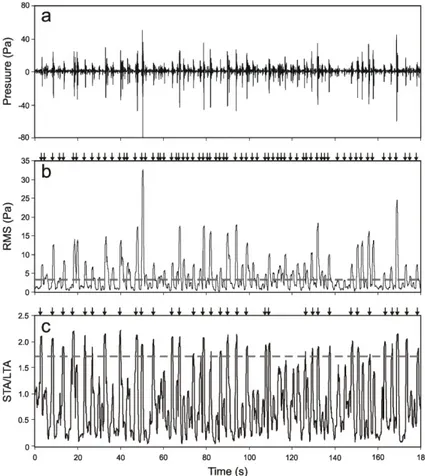
4.2 Events triggering 106

4.3 Averaged multi-channel coherence 110

4.4 Seismo-volcanic events source location 112

4.5 Volcanic tremor location and errors estimate 117

4.6 Three component sensor analysis 121

4.7 Waveform similarity detection 125

5. Infrasonic signals on active volcanoes 129

5.1 Infrasound monitoring at Mt. Etna 133

5.2 Source mechanism 140

5.2.1 Resonating conduit 143

5.2.2 Strombolian bubble vibration 144

5.2.3 Helmholtz resonator 147

5.3 Infrasound investigation at Mt. Etna during

September-November 2007 as a case of study 154

5.3.1 Source location 163

5.3.2 Source mechanism 166

5.3.3 Emitted gas volume 169

5.3.4 Volcanic activity 173

5.4 Mt Etna during May 2008: second

case of study 176

5.5 Clustering of infrasonic events as tool to detect and locate explosive activity at

Mt. Etna volcano 186

5.5.1 Discovering clusters using SOM 187

5.5.2 Real time infrasound signals

classification system 190

6. Insights into deep volcano dynamics using

seismo-volcanic signals 199

6.1 Seismic signals on active volcanoes 200

6.2 Seismo-volcanic signals at Mt. Etna

during 2007 207

6.2.1 Signal analysis 211

6.2.2 Tremor source location 213

6.2.3 Waveform events classification 217

6.2.4 Properties of the resonator system 221

6.2.5 Events location 222

6.2.6 Volcanic processes 226

6.3 Seismo-volcanic signals at Mt. Etna

6.3.1 VT earthquakes, ground deformation and

volcanic tremor 232

6.3.2 Long period events 236

6.3.3 Infrasound and LP events as precursor 242

6.4 Discover lava fountain precursors using

three component sensors 246

6.5 Multi-stations coherence 251

6.6 Seismic and infrasonic coupling using cross-

wavelet analysis 254

6.7 Banded tremor phenomena at Mt. Etna

during 2008 260

6.7.1 Banded tremor characteristics 262

6.7.2 Spectra and polarization analysis 265

6.7.3 Tremor source location 270

6.7.4 Comparison between seismic and

infrasonic OSA patterns 276

6.7.5 Nonlinear analysis of banded tremor 279

6.7.6 Banded tremor qualitative model 285

7. Conclusions 291

References 295

Chapter 1

Volcano monitoring

Monitoring of active volcano uses a wide range of techniques and instru-mentations. Its aim is the interpretation of data in order to discover pat-tern in geophysical and/or geochemical parameters before, during and after eruptions. Monitoring provides the means to answer questions of vital interest to communities affected by impending eruptions such as when and where will the volcano erupt? Which areas are safe or danger-ous? When will the eruptions cease? (McNutt et al., 2000). The answers come from an optimal interpretations of data and give information for forecast purpose. Unfortunately, the capability to answer these questions depends on the adequate scientific understanding of complex volcano dy-namics both in general and for each specific volcano. A primary role in volcano monitoring is to establish the level of background or baseline ac-tivity of each monitored parameter, against which anomalous acac-tivity can be measured (McGuire, 1991). Well-equipped and well-staffed volca-nological observatories are located only close to 20 of the potentially eruptive volcanoes and some geophysical instruments (most seismome-ters and benchmarks of geodetical networs) are installed on about 150 volcanoes in the world (Scarpa and Gasparini, 1996). Changes in geo-physical and geochemical pattern are indicative of possible eruptive reac-tivation and include

Figure 1: Techniques for volcano monitoring (modified from McGuire, 1991).

Acronyms: EMR: electro-magnetic radiation; EDM: electronic distance measure-ment; GPS: global positioning system; SAR: synthetic aperture radar; IR: infra-red; SP: self-potential; ER: electrical resistivity; COSPEC: correlation spectrome-ter.

changes in seismicity, ground deformations, physical-chemical changes in fumaroles, emission rates of volcanic gases, anomaly in

gravity and magnetic fields. When combined with geological mapping and dating studies to reconstruct comprehensive eruptive histories of high-risk volcanoes, these geoindicators can help to reduce eruption-related hazards to life and property. Different techniques are used to monitor these parameters (figure 1). Each type of data provides informa-tion related to process which may be related to movement of molten rock or other precursory phenomena. Seismic activity is considered one of the best indicator of the evolution of volcanic activity and is one of the most common surveillance tool for active volcano.

The seismology gives useful information about the location of magma bodies/hydrothermal fluids in depth, their dynamics and composition and the plumbing system geometry (e.g. Kumagai and Chouet, 1999; Chouet et al., 2003; Patanè et al., 2006). Moreover, most volcanic eruptions have been preceded by increases in earthquake activity beneath or near the volcano (McNutt, 1996 ). Once the background seismicity has been char-acterized for a particular volcano, changes in the “steady state” may be related to changes in the volcano activity. Ground deformation study is another technique for volcano monitoring. Generally, the movement of subsurface material precedes volcanic eruptions and the increasing pres-sure results in ground deformation (Van der Laat, 1996). It is possible to model deformation caused by change of volume at a certain depth and modeling magma reservoirs, cracks and conduits (e.g. Van der Laat, 1996; Linde et al., 1993). GPS is the most suitable technique to measure ground deformations. However, it provides spot data, i.e. they refer to network vertices whose number rarely exceeds the order of tens in areas of hundreds, often thousands, of square kilometers (Palano et al., 2008). Remote sensing is a growing field in volcano monitoring and provides the only practical monitoring tools for many volcanic areas that are in rela-tively isolated regions. As defined in Francis et al. (1996), remote sensing consists of detection by a sensor of electromagnetic energy reflected, ra-diated or scattered from the surface of volcano or its airborne erupted material. For volcanoes already monitored by conventional techniques, this technique not only provides complementary observations but also offers new approaches (e.g. monitoring of ground deformation using In-SAR techniques). Electromagnetic variations, preceding eruptive or seismic activity, are sometimes observed in volcanic areas (e.g. Johnston et al., 1981). Microgravity studies, involving the measurement of small changes with time in the value of gravity at a network of stations with

respect to a fixed base, are a valuable tool for mapping out the subsurface mass redistributions that are associated to volcanic activity (Rymer, 1996). Volcanic gas analysis and temperature measurements are also commonly performed. While geophysical precursors may yield different patterns related to the particular volcanic system, tectonic setting and physicochemical properties of the magma, geochemical precursory mostly depends on changing rates of magma degassing and interactions with shallow aquifers (Martini, 1996). Significant variations have been ob-served prior to some eruptions but often the changes occurred with the onset of the eruption (McNutt et al., 2000). Although these techniques have been successfully applied to forecast eruptive events on different volcanoes, during the last years new insights into explosive volcanic processes have been achieved by studying infrasonic signals (e.g. Vergni-olle and Brandeis, 1994; Ripepe et al., 1996, 2001a). This kind of signal, together with seismic signal related to volcanic processes, constitutes an useful tool able to significantly contribute to volcano activity monitoring.

1.1 Volcano seismology

Seismic sources at volcanoes are highly complex and involve gases, melts and solids interaction (McNutt et al., 2000). Volcano seismology is a field of volcanology in which seismological techniques are employed to under-standing physical conditions and dynamic states of volcanic edifices and volcanic fluid systems (Kawakatsu and Yamamoto, 2007). The main goal of volcanic seismology is to understand the nature and dynamics of seis-mic sources associated with the injection and transport of magma and related hydrothermal fluids (Chouet, 2003). Active volcanoes are the sources of a great variety of seismic signals. Traditionally, seismo-volcanic signals have been classified into six different types: high-frequency (HF) and low-high-frequency (LF) events, Very Long Period (VLP) events, volcanic tremor, hybrid events and volcanic explosions (figure 2) (e.g. Minakami, 1974; Lahr et al., 1994; McNutt, 1996; Zobin, 2003; Iba-nez et al., 2003):

HF events: high-frequency events, also called Volcano Tectonic events

(VT), manifest clear onset of P- and S-wave arrivals. In general, they are subdivided into two classes: deep VT events (VT-A), located below about 2 km, that manifest high frequency content (> 5 Hz); VT of type B (VT-B) that show much more emergent P-wave onset and sometimes any clear S-wave arrival and their spectral bands are shifted to lower fre-quencies (< 5 Hz) (Wassermann, 2009). High frequency may be generated at the source, but is not recorded because of instrumental limitations or high local attenuation (McNutt, 1996). HF events have been attributed to regional tectonic forces, gravitational loading, pore pressure effects and hydrofracturing, thermal and volumetric forces associated with magma intrusion withdrawal, cooling, or some combinations of any or all of these

(McNutt, 2005). This kind of events differ from their tectonic counterpart only in their patterns of occurrence, which, at volcanoes, are typically in swarm rather than mainshock-aftershock sequences (McNutt, 1996). HF events are useful at volcanoes to determine stress orientation via study of focal mechanisms and stress tensor inversion (e.g. Moran, 2003; San-chez et al., 2004; Waite and Smith, 2004). The greatest progress in study VT events has been the implementation of new techniques for defining the volcanic structures; in particular, high-resolution tomography is a powerful method for determining subsurface volcanic structure (e.g. Dawson et al., 1999; Patanè et al., 2006).

LF events: Low-frequency events (LF), also called long period events (LP)

(figure 2b), commonly observed on many volcanoes worldwide, are be-lieved to be caused by fluids moving in volcanic conduits, heat and gas supply (Chouet, 1996a; Almendros et al., 2002a) and considered precur-sory phenomenon for eruptive activity. LP signals show no S-wave arriv-als and very emergent signal onset. LP sources are often shallow (< 2 km) and their frequency content is mostly restricted in a narrow band between 0.5-5 Hz. LP activity originates in particular locations within the magma plexus where disturbances in the flow are encountered (Chouet, 1996a). Despite the ambiguity regarding the source, many au-thors have studied these events, focusing on particular features such as spectral content, rates, or relation to eruptions (McNutt, 2005). Injection of water into hot dry rock has been found to produce seismic signal simi-lar to LF volcanic signal and support the idea of a source that involves the opening of tensile cracks caused by excess fluid pressure (Bame and Fehler 1986; Konstantinou, 2002). The associated source models range from an opening and resonating crack (Chouet, 1996a; Wassermann, 2009) to existence of pressure transients within the fluid-gas mixture

causing resonance phenomena within the magma itself (Wassermann, 2009; Seidl et al., 1981). Since LF events exhibit no emergent onset, phase picks are difficult to determine, thereafter it is impossible to apply standard location algorithm based on travel time inversion. Recently, LF events are located using semblance location techniques from particle mo-tions recorded on a broad-band seismometer network (Kawakatsu et al., 2000).

Hybrid events: Some seismo-volcanic signals show characteristics of both

LF and HF events and are called Hybrids (figure 2d). They are consi-dered a subset of LF earthquakes, characterized by high-frequency on-sets. Signals of this class begin with high-frequency phase followed by monochromatic signal which may reflect a possible mixture of source me-chanisms. Spectral analysis reveals the different properties of these two distinct phases. The initial high-frequency portion has a broad spectrum, extending up to frequencies of 40 Hz. In contrast, the LP segment is qua-si-monochromatic and peaks at low frequencies (1-6 Hz) (Ibanez et al., 2003). These events are thought to represent the failure of brittle rock which is accompanied by the excitation of nearby magmatic fluids. Some studies suggest that the onsets represent a separate trigger that initiates conduit resonance (Neuberg, 2006). Events of this sort have been ob-served at different volcanoes such as Montserrat, Redoubt, and Decep-tion Island (Lahr et al., 1994; Miller et al., 1998; Neuberg et al., 2000; Ibanez et al., 2003).

Explosion quakes (ExQ): This signal class accompanies Strombolian or

other explosive eruptions (figure 2e). Most of these signals can be identi-fied by the occurrence of an air-shock phase caused by the sonic boost during an explosion (Wasserman, 2009). Some LF events show the same

frequency-time characteristics but lack an air phase (McNutt, 1986) re-flecting a common source mechanism of deeper situated LF and shallow produced explosion. They have been studied by using calibrated infrason-ic minfrason-icrophones or infrasoninfrason-ic pressure sensors. Key issues include the depth, ground-air energy coupling and seismic or acoustic efficiency (McNutt, 2005). The infrasonic signal (figure 2f) for short distances tra-vels in an almost homogenous atmosphere without structures that may scatter, attenuate or reflect acoustic waves. Then, unlike the seismic sig-nal whose wavefield is strongly affected by topography (Neuberg and Pointer, 2000) and path effects (Gordeev, 1993), the infrasonic signal maintains its features almost unchanged during propagation, allowing obtaining information concerning source dynamics. This can be explained by the simpler Green’s functions for a fluid atmosphere than those for a complex, heterogeneous volcanic edifice, which supports compressional, shear, and surface waves (Johnson, 2005). Thus acoustic data give a more direct view of some explosive and eruptive processes (McNutt, 2005). The source mechanism of the sound radiated during eruptions is still open to debate. According to some studies, this signal can be related to the acoustic resonance of magma in the conduit, triggered by explosive sources, implying propagation of sound waves in the magma and atmos-phere through an open vent (Buckingham and Garces, 1996; Garces and McNutt, 1997; Hagerty et al., 2000; Cannata et al., 2009a). Other theo-ries relate the source of sound to eruption dynamics, such as a sudden uncorking of the volcano (Johnson et al., 1998; Johnson and Lees, 2000), local coalescence within a foam (Vergniolle and Caplan-Auerbach, 2004) and Strombolian bubble vibration (Vergniolle and Brandeis, 1994, 1996; Vergniolle et al., 1996, 2004). Methods to estimate relative elastic energy partitioning during Strombolian eruptions were developed and show var-iations related to changing vent conditions (Johnson and Aster, 2005).

Figure 2: waveforms with the associated spectrograms for: (a) VT earthquake

(VT); (b) long period event (LP); (c) volcanic tremor; (d) hybrid event (Hyb); (e) ex-plosion quake (EXQ); (f) infrasonic signal.

Very Long Period Events: the use of broadband seismometers in the past

decade has allowed to record a new class of seismo-volcanic signals called Very Long Period (VLP) events. VLP events with dominant periods in the range 2–100s (Neuberg et al., 1994; Ohminato et al., 1998) are assumed to be linked to mass movements, and to represent inertial forces result-ing from perturbations in the flow of magma and gases through conduits (Uhira and Takeo, 1994; Kaneshima et al., 1996; Chouet, 1996b; Cannata et al., 2009c). This class of signals has been observed at several volcanoes such as Aso Volcano (Kawakatsu et al., 1994; Kaneshima et al., 1996; Yamamoto et al., 1999), Stromboli (Neuberg et al., 1994; Chouet et al., 2003), Kilauea (Ohminato et al., 1998), Etna (Cannata et al., 2009c; Patanè et al., 2008).

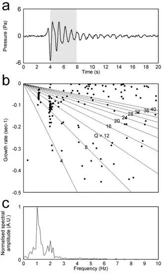
Volcanic tremor: volcanic tremor is a persistent ground vibration

record-ed near active volcanoes (figure 2e). In figure 3 is shown a location of vol-canoes where the tremor occurrences were recorded (Konstantinou and Schlindwein, 2002). This signal is the most favored parameter in volcano early eruption warnings. At Mt. Etna (Italy), strong fluctuations of vol-canic tremor amplitude are associated with lava fountaining or with opening of a flank fissure (Cosentino et al., 1989). Tremor is generally characterized by narrow frequency range and long duration compared with earthquakes and other seismo-volcanic signals (figure 2e). Although spectra of tremor usually contain a series of narrow peaks suggesting the modes of oscillation of a resonant system, commonly tremor signal is complicated and chaotic in appearance (Julian, 1994). Seismo-volcanic earthquakes like LP and explosion quakes events have spectra similar to tremor and probably are closely related to it. Observations made at dif-ferent volcanoes suggest the involvement of gas/fluid interaction.

Figure 3: Location of volcanoes that present tremor occurrence (from

Konstanti-nou and Schlindwein, 2002 )

The content spectra similarity with LP and ExQ signals suggests a simi-lar source process. Flow instability plays an important role in the excita-tion of volcanic tremor in multi phase flow pattern (Seidl et al., 1981; Schick, 1988) and associate LP and ExQ are seen as a transient within the same physical process (Wasserman, 2009). The physical mechanism of the tremor source has proved to be very difficult. Complexity arises from the fact that a volcano represents the place of interaction between material of different physical properties: magmatic fluids, surrounding bedrock and gases (Konstantinou and Schlindwein, 2002). It is well known that very different physical processes in a volcano may produce quite similar results (Schick, 1992). This has been confirmed by theoreti-cal modeling in the frequency domain of tremor and low frequency

seis-mo-volcanic events and was found that many physical mechanisms could explain them equally well (Nishimura et al., 1995). Also, many authors support the fact that the tremor source is not unique and may differ from a volcano to another. Harmonic tremor and spasmodic tremor are two special cases of more general volcanic tremor.

Figure 4: Tremor gliding phenomena . The changing frequency content with time

The former is a low-frequency, often monotonic sinusoid with smoothly varying amplitude, the latter is a higher-frequency, pulsating and irregu-lar signal (Finch, 1949; McNutt, 1996). A very interesting feature of tre-mor is referred to as gliding (figure 4), in which the frequencies of evenly spaced spectral peaks vary systematically with time. Also in the case of the volcanic tremor, the standard location techniques based on travel time inversion cannot be used because of the non-impulsive signature of tremor. Therefore, new methods based on the space distribution of the seismic amplitude were developed and used for the signals coming from classical seismic networks (different techniques are used for the seismic arrays) (Battaglia and Aki, 2003; Di Grazia et al., 2006). A large number of papers showed a strict relationship between eruptive activity and variations of volcanic tremor. They consist of whether spectral and am-plitude changes (Gresta et al., 1991; McNutt, 1994; Alparone et al., 2007; Cannata et al., 2008) or location source variations (Patanè et al., 2008; Di Grazia et al., 2009).

1.2 Time Series Analysis: an introduction

Time series (TS) problems arise in almost all disciplines, ranging from studying variations in biomedical measurements to variations in geo-physical or in financial parameters. A time series is a finite series of ob-servations usually collected at regular intervals. Using time series analy-sis it is possible to characterize, predict and model the observed system. Also, time series obtained by different disciplines (e.g. geophysics and geochemistry) can be analyzed in order to discover a possible link among them. Once the background level has been characterized, changes in the so called “steady state” may be related to changes in the activity.

From a seismo-volcanic point of view, several parameters can be ex-tracted from recorded signals. Since they are linked to magma-gas mo-tion inside the volcano, studies of changes in parameters like spectral content, rate, quality factor, background noise and wavefield, can be used for understanding volcano dynamic evolution and their implications for monitoring purposes. In order to accomplish this task, time series analy-sis (TSA) techniques provide useful tools for volcano state changes inter-pretation. In TSA there are three recurring main tasks (Gershenfeld, 2006). The first task is related to nature of the underlying system that produces observed time series. It provides information about the nature of the system, its degrees of freedom, its linear or nonlinear nature, noise influences and how random it is. The second task is related to forecast defined as the estimation of the next state known the current state. The last task is the TS modeling and is related to governing equations esti-mation and their long-term behavior.

Regression analysis: Linear system theory is expressed by the Wold

de-composition where a stochastic process is separated into the sum of two processes: deterministic one that is a linear function of its past values; stochastic one that is a linear function of previous values of uncorrelated random variable (Priestley, 1981; Gershenfeld, 2006). Approximation of Wold form with finite number of parameters leads to auto-regressive/moving-average (ARMA) process where the system output y is a linear function of external inputs x, its previous outputs and noise. Al-though linear systems are very well understood, they appear very limited in real geophysical applications where non-linearities are significant.

Stationarity: Traditional time series analysis implicitly assume that data

come from a linear dynamical system with many degrees of freedom and added noise. The variation is assumed to be a superposition of sine waves and additional terms that grow or decay. The exponential terms typically lead to nonstationarity in which statistical properties of time series, such mean or standard deviation, change in time (Sprott, 2003). In time series measurement, reproducibility is closely connected to the stationarity of the underlying process (Kantz and Schreiber, 1997). The weakest statio-narity requires that probably density functions (p.d.f.) remain constant for all parameters that characterize the dynamic of the system. A time series is considered to originate from a stationary process if statistical fluctuation of mean, variance and auto-covariance, does not change over time. In order to estimate the stationarity, some methods use nonlinear statistics techniques, such as the so-called cross-prediction error (Schrei-ber, 1997).

Non-linear analysis: Link between chaos theory and real world is the

that real processes are characterized by a number of interdependent va-riables. Modeling of geophysical/geochemical systems is an extremely dif-ficult task. Data sequences are obtained from the observation rather than physical equations. For a dynamical description of such time series, linear statistical techniques are insufficient as they do not take into ac-count nonlinear relationship (Matcharashvili et al., 2000). A nonlinear dynamical approach provides more information on complex system beha-vior than classical linear tools (Berge et al., 1984; Theiler, 1990; Abarba-nel et al., 1993; Kantz and Shreiber, 1997). Theory of deterministic chaos is an useful tool in order to explain irregular behavior of systems that are not influenced by stochastic inputs. The dynamics of systems is described in state space, whose dimension is given by the number of the dependent variables of the model. State space describes how the behavior of a nonli-near system evolves as one or more of its parameters are bifurcating (Konstantinou and Lin, 2004). When we analyze a time series, we will almost always have only incomplete information due to the measurement on a single variable as a function of time. In this cases the state space and the dynamics of the system that generated the measures are un-known. The missing information can be recovered from time delayed cop-ies of the available time sercop-ies if certain requirements are fulfilled (Schreiber, 1998). Several geophysical systems exhibit chaotic behavior characterized by high sensitivity to initial conditions. Small changes in initial conditions or slightly different external forces produce wildly dif-ferent outcomes even when the governing equation are known. Nonlinear time series analysis provides practical method for studying chaotic sig-nals by reconstructing phase space and extracting information about the underlying process.

Time-frequency analysis: In time series analysis we can represent

inmation in two basic ways: time and frequency representations. The for-mer does not display spectral content while the latter shows only fre-quency information. Frefre-quency representation is commonly computed using the Fourier transform that allows the retrieval of information on power content at any frequency. The widely used Fourier transform is designed for stationary signals; in classical Fourier analysis we lose the frequency location in the time domain. For the analysis of time series containing non-stationary power at many different frequencies, Short time Fourier transform (STFT) and wavelet transform (WT) are common-ly applied (Daubechies, 1990). In contrast to the Fourier transform, which consists of a linear superposition of independent and nonevolving periodicities, the WT is based on the convolution of signals with a set of functions derived from the translations and dilatations of a basic func-tion called the “mother wavelet”. Unlike STFT, WT gives a more accurate time-frequency description of signals containing low and high frequency components. Taking into account STFT method, once the length of the moving window is chosen, also the frequency resolution is fixed, and the entire phase space is uniformly described by cells of fixed sizes. Con-versely, WT method, based on variable-sized cells, allows the use of long time intervals to gather more precisely low-frequency information, and of shorter regions for high-frequency information (Bartosch and Seidl, 1999; Lesage et al., 2002). Some example of time-frequency representation of seimo-volcanic events are reported in figure 2 and 4.

1.3 Pattern recognition approach

The process of automatic extraction, recognition, description and classifi-cation of patterns extracted from time series plays an important role in modern volcano monitoring techniques. In particular, the ability of a cer-tain system to recognize different volcano regimes can help the research-ers to better undresearch-erstand the complex dynamics underlying the geophysi-cal systems. The recognition process consists of one of the following tasks: supervised classification and clustering. Clustering and classifica-tion processes in high dimension metric space are widely applied on data analysis when more than two descriptive features are needed. For this purpose approaches based on Self Organizing Map and density based method will be illustrated. Also, the classification problem by optimal hyperplane separator using support vector machine (SVM) will be faced with the aim of classifying information provided by the clustering task. A basic pattern recognition schema is shown in figure 5 and can operate in two modes: training mode and classification mode (Jain et al., 2000).

The role of the preprocessing module is to segment and filter the pattern of interest from the background, remove noise, normalize the pattern and then comprises all the operations used to define a compact representa-tion of the pattern. In the training mode, the features extracrepresenta-tion block finds the descriptive features of the input patterns and then the classifier is trained to partition the features space.

Chapter 2

Time series analysis methods

In this chapter methods for time series analysis will be introduced. In particular, we will focus on the time-frequency domain signal processing and nonlinear analysis techniques. The former techniques are related to multi-scale/frequency signals representation using wavelet framework considering statistical significance with respect to a background noise. Further, a brief description of power parametric spectrum estimation will be introduced. The nonlinear techniques will be treated to investigate time series from a dynamical point of view. In particular, various meth-ods for determinism and nonlinearity detection will be applied in order to characterize different kinds of signals. A very important topic will be the chaotic behaviour detection and phase space reconstruction from a single time series. This methodology has been widely applied since the available data are generally in form of time series and the underlying dynamical system in unknown. All of these techniques will be applied in the next chapters with the aim to investigate different volcano activity regimes at Mt. Etna volcano.

2.1 Time-Frequency analysis

Information content of a physical quantity can be represented either as a function of time (time domain) or as a spectrum (frequency domain). A function of time does not show spectral content while representation by Fourier spectrum cannot represent the temporal variation of the signal. The Fourier transform give information about the spectral content of a signal using a linear superposition of independent and non-evolving peri-odicities. This technique implicitly assumes that the underlying process is stationary and gives no information about the location of these fre-quency in time. This treatment is not well suited for data which involves transient process and frequency content changes in time. Fourier analy-sis presents limitation if applied on signals including intermittent burst processes or intermittent processes (Labat, 2005). To overcome this prob-lem methods based on sub-sections or moving-windows of the data are used in order to detect abrupt regime changes in statistical property of the signal. Common approaches in time-frequency analysis are the Win-dowed Fourier Transform (WFT), also known as Short Time Fourier Transform (STFT), and Continuous Wavelet Transform (CWT). These representations give a very clear picture of the non-stationarity nature of the signal in a time-frequency domain. STFT provides this representa-tion by transforming short windows of data. In this case a Fourier spec-trum is computed over time by a fixed-size window shifted along the time axis. This has the problem that a fixed size moving window limits the de-tection of cycles at wavelengths that are longer than windows itself, and nonstationarity in short wavelength are smoothed (Prokoph and Patter-son, 2004; Gershenfeld, 1999). The use of CWT solves this problem be-cause it uses wide windows at low frequencies and narrow window at high frequencies providing a multi-scale representation of the signal.

2.1.1 Short Time Fourier Transform

STFT is defined as a convolution between a signal f(t) and a sliding win-dow w(t-t’):

  

'

'



'

)

,

(

_t

_f

_t

_w

_t

_t

_e

_dt

S









where w*(t-t’) is the window function centered on t, commonly a Hann or Gaussian window (Bartosch and Seidl, 1999; Lesage et al., 2002). STFT can be seen as a local spectrum of f(t’) around the analysis time t, whose position indicate the approximate time for which the spectrum is valid. STFT of a sequence f(n) is defined as:

n j n

e

n

m

w

n

f

m

F

_







(

)

(

)

)

,

(

where the sequence f(n)w(m-n) is called short-time section of the se-quence f(n) at time m. The windowing process introduces leakage effects and frequency resolution strongly depends on the choice of the window function. In particular, time-frequency resolution can be adjusted by the window length tw. A good time resolution requires a narrow window in

time, while a good frequency resolution requires a large window in time (corresponding to a narrow filter in frequency domain). Once the window size is chosen, both time and frequency resolutions are fixed and the en-tire phase space is described by cells of fixed size (figure 1).

Fig. 1: Filtering view of STFT at frequency ω0.

This is related to Heisenberg’s uncertainty principle that prohibits the existence of a window with arbitrary small duration and bandwidth. Once the windows size tw is chosen, the smallest measurable frequency is

determined as fw=1/tw (Lesage et al., 2002; Bartosch and Seidl, 1999).

Equation (2.1) can be interpreted as a convolution between the signal f(t) and the window function w(t) also called analysis filter. The last defini-tion is justified on the basis of the fact that STFT can be interpreted as the output of an infinite channel of filter bank where the window w(n) plays the role of the filter input response (Nawab and Quatieri, 1988). Fixing ω= ω0 equation (2.2) can be rewritten as:







_



_w

_m

_n

e

n

f

m

F

(

,

)

(

)

(

)



Using the convolution operator * equation (2.3) can be rearranged as:



(

)



(

)

)

,

(

m

f

n

e

w

m

n

F

_

_

_

_

The term _f(n)ej0ncan be interpreted as modulation of f(n) up to the

fre-quency ω0.

In the light of it equation (2.4) can be rewritten in the following form:     





e

n

w

n

f

e

n

F

(

,

)

(

)

(

)







a block diagram as shown in figure 2  (Nawab and Quatieri, 1988; Bar-tosch and Seidl, 1999).  Considering a finite number of frequencies the STFT can be viewed as the output of the filter bank shown in figure 2 where each filter is a bandpass filter centered around its selected fre-quency ωi (i=0..N-1).

Figure 2: STFT as the output of a bandpass filter bank.

2.1.2 Continuous Wavelet Transform

As aforementioned, STFT has the drawback of fixed resolution in time-frequency domain. In general it is very difficult to find a good trade-off between frequency and time resolution. The continuous wavelet trans-form (CWT) solves this problem because it combines high temporal reso-lution with good frequency resoreso-lution offering a reasonable balance be-tween these two parameters. For this reason CWT is an useful tool when signals are characterized by localized high frequency or scale-variable process and allows tracking time evolution at different scales (Labat, 2005; Leasage et al., 2002). The CWT transforms the signal in a time-scale plane called scalogram. From a mathematical point of view it is de-fined as:

'

'

)

'

(

1

)

,

(

_dt

a

t

t

t

f

a

a

t

W











 







where ψ is a real or complex function called analyzing wavelet, a is the dilatation parameter which controls the time duration of the wavelet and

t is the translation parameter. The analyzing wavelet fulfills the

admis-sibility condition:

 

















d

0

 

_

 







_

t

e

dt

is the Fourier transform of ψ(t) (Daubechies, 1992; Bartosch and Seidl, 1999). Let a discrete sequence x(n) (n=1,..,N), the CWT can be defined as:

  











 





a

t

n

n

n

x

a

n

W

_'

'

)

,

(



where δt is the uniform time step, * indicates complex conjugate, a is the wavelet scale and N is the number of points in the time series. By trans-lating the time index n and varying the scale a we obtain a picture show-ing amplitude at any scales and its variation with time. The convolution in equation (2.9) can be computed faster in the Fourier space. The DFT (Discrete Fourier Transform) of the sequence x(n) is defined as:

 

x

n

e

N

X

1





with frequency index k=0…N-1. Using the convolution theorem, wavelet transform can be viewed as the inverse Fourier transform of the product:

 

 

e

a

X

a

n

W

_

_

ˆ

,





where the angular frequency is defined as:























2

:

2

2

:

2

N

k

t

N

k

N

k

t

N

k











Figure 3: CWT as non-uniform infinite channel filter bank.

and Ψ _{is the Fourier transform of the wavelet function Ψ / .}

The choice of wavelet function (also called mother wavelet) is a critical aspect of the CWT and it is related to the particular features that we want to consider in our analysis (Torrence and Compo, 1998; Farge, 1992). One particular wavelet, used in time series feature extraction, is the Morlet wavelet that provides a Gaussian modulation of the time-scale plane:

 









e

e

where ω0 and η are the dimensionless frequency and time respectively (Grinsted et al., 2004). In order to provide a good balance between time and frequency and satisfy the admissibility condition ω0 must be 6 (Farge, 1992). It is noteworthy that for Morlet wavelet ( with ω0=6 ) the Fourier period T is almost equal to the scale ( T ~ 1.03a ). In order to

normalize the CWT that is to have unit energy, equation (2.9) can be written as:

  









Similar to STFT (section 2.1.1), the CWT can be investigated as a non-uniform infinite channel filter bank (figure 3). In this case impulse re-sponse is derived by dilatation of prototype band pass impulse rere-sponse Ψ(n) whose duration depends on the scale parameter a (Bartosch and Seidl, 1999). Transferring concepts of classical Fourier analysis to wave-let domain, a wavewave-let power can be defined as the transformation of the autocorrelation function. Since the wavelet function Ψ(n) is in general complex the W(n,a) is also complex. The transform can be divided into real part R{W(n,a)} and imaginary part I{W(n,a)} and amplitude |W(n,a)|, and phase, tan-1_{[I{W(n,a)}/R{W(n,a)}]. The Wiener-Khinchin}

theorem can be defined as the expectation value of W(n,a) multiplied by its conjugate: ) , ( ) , ( ) , (_{n a} 2 _{W n aW}* _{n a} W  (2.15)

If wavelet is centered close to the beginning or to the end of the time se-ries, edge artifacts occur. For this reason it is useful to introduce the so called Cone of Influence (COI) in which edge effect become important and the results should be interpreted carefully. COI can be defined as the area in which the wavelet power caused by a discontinuity at the edge has dropped by a factor e-2 _{of the value at the edge itself (Torrence and} Compo, 1998; Grinsted et al, 2004; Maraun and Kurths, 2004).

2.1.3 Comparison between STFT and CWT

Both time-frequency methods can be interpreted as the inner product of the signal f(t) and a function F(t,f). In the case of STFT the F(t,f) takes the form: ' 2

)

'

(

)

,

(

_t

_f

_g

_t

_t

_e



_

_











 



a

t

t

g

f

t

,

)

'

(



Both techniques have the same time-frequency resolution limitations. While STFT resolution do not depend on the investigated frequency (the window size is fixed a priori) the CWT is a multi-resolution approach with better time resolution at high frequency and better frequency reso-lution at low frequency. The tilling of the time-frequency plane is differ-ent for both STFT and CWT and is characterized by duration T and bandwidth B. In the former these two parameters are constant (T=const, B=const) and the tiled time-frequency plane can be represented as in fig-ure 4a. In the latter case the parameters T and B are related to the scale

parameter a (T=a, B=Ba=1/a) and lead to a non uniform tile

time-frequency plane (figure 4b). An example of time-time-frequency representation of a signal with added spike and noise using STFT and CWT is shown in figure 5.

Figure 4: Tilling of time-frequency plane of a) STFT and b) CWT.

Figure 5: STFT (middle plot) and CWT (bottom plot) of a synthetic signal (top

plot) of Gaussian windowed 5 Hz harmonic signal with added spike and noise. The spike and the beginning of the high frequency noise is well resolved in time by CWT than STFT. This picture clearly shows the advantages of CWT respect to classical spectrogram based on Fourier transform.

2.1.4 Statistical significance

In order to estimate the reliability of the power spectrum a statistical significance level is required. To accomplish this task one firstly needs an appropriate hypothesis about background spectrum.

Statistical significance of power spectrum is based on the assumption that the investigated signal is generated by a stationary process with a given background power spectrum. This assumption is known as the null

hypothesis. Hypothesis about an appropriate background spectrum is

closely related to the considered system. For many geophysical pheno-mena background spectrum can be white noise (flat Fourier power spec-trum) or red noise (increasing power with decreasing frequency). The last one reflects the fact that a sort of memory is presented in the process that generates the measured signal. A simple method for red noise mod-eling is an AR1 (auto-regressive model of first order) process with lag-1 autocorrelation α:

n n n

x

z

x







with x0 = 0, and zn is taken from Gaussian white noise (Torrence and

Compo, 1998). Fourier power spectrum of (18) is given by (e.g. Allen and Smith, 1996): 2 2 2

1

1

e

P











where k is the Fourier frequency index. Let a time series and a back-ground spectrum hypothesis, the estimated power spectrum peak above background spectrum can be assumed to be a true feature with a certain percent confidence. Peaks in the time series power spectrum are assumed

significant if they exceed the 95% confidence spectrum computed based on the hypothesis of white or red background noise. For definition the ‘95% confidence’ level is equivalent to ‘significant at the 5%’ and ‘95%

con-fidence interval’ is related to the range of concon-fidence about a given value.

If a time series xn is normally distributed, both real and imaginary part

of the DFT coefficients Xk are normally distributed (Chatfield, 1989).

Since the square of normally distributed variable is chi-square distri-buted with one degree of freedom then | | is chi-square distridistri-buted with two degree of freedom denoted by (Jenkins and Watts 1968). For instance, to obtain 95% confidence level, the background spectrum given by equation (2.19) must be multiplied by the 95Th percentile value for 2

2

 (Gilman et al., 1963; Torrence and Compo, 1998). Under the as-sumption of a background noise given by equation (2.19), the distribution of normalized Fourier power spectrum can be expressed as:

2 2 2 2 2 1 ˆ





The corresponding relation in wavelet domain at each scale a and time n is:

 

2

1

,





P

a

n

W

Dist

_

















These relations are correct assuming that the underlying distribution of the original time series is Gaussian. The choice of the mother wavelet is very important in the definition of wavelet power. As explained in Ge (2007) the wavelet power has a distribution only when a wavelet

fam-ily used is the Morlet wavelet. In practice, for many time series an ana-lytical expression of the significance level against red-noise null hypothe-sis is not available. In this case the significance level can be obtained empirically through Monte Carlo simulations (e.g. Torrence and Compo, 1998; Grinsted et al., 2004). More details about wavelet significance test can be found in Ge (2007,2008).

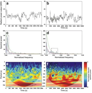
Figure 6:(a and b) Time series of the radiant power output of thermal camera;(c and d) powerspectra computed via periodogram normalized by standard deviation of the time series shown in Figures 6a and 6b; (e and f) Wavelet transform, com-puted using a Matlab code provided by Grinsted et al., 2004, of the two time se-ries.

Methods described in this section have been widely applied on different scientific research areas, such as geophysics, volcanology and seismology. In figure 6 an application of Fourier and Wavelet power spectrum esti-mation together with the confidence level is shown. The two time series reported in figure 6a and 6b, were obtained from thermal image (Spam-pinato et al., 2008). Both time series were normalized with 0 mean and unit standard deviation before wavelet spectrum computation. In order to investigate the most energetic periods, classical Fourier transform (figure 6c and 6d) and wavelet transform (figure 6e and 6f) were applied. Peaks in power spectrum are assumed significant if they exceed the 95% confidence spectrum computed based on the hypothesis of red back-ground noise. Peaks found using periodogram (figure 6c and 6d) are con-sistent with the wavelet transform results (figure 6e and 6f), which show significant spectral power (highlighted by the solid contour at 95% confi-dence interval). Also the cone of influence (COI) discussed in section 2.1.2 is shown in figure 6e and 6f.

2.1.5 Cross-spectrum and coherence

Let x(t) and y(t) two ergodic and stationary processes, the cross-correlation can be considered as a quantitative measure of the related-ness of two signals. The Fourier cross-spectrum can be defined as (Labat, 2005):













i

f

d

R

f

S







(

)

exp

2

)

(

where RXY(τ) is the cross-correlation between the signals x and y. SXY is

autospectra of the two signals X and Y respectively. Coherence is an ex-tension to Pearson’s correlation coefficient and can provides a measure of the linear relationship between two signals at various frequency (Saab et al., 2005; Caviness et al., 2003). In the light of it, spectral coherence can be defined as:

 

 

   

Using Schwarz inequality we observe that CXY(f) takes values between 0

and 1. The aforementioned Coherence measure assumes stationary of the signals and, similarly to Fourier transform, is insensitive to changes over time. To overcome this problem, a STFT (see section 2.1.1) approach is applied to produce the coherogram. In practice, while with Fourier cohe-rence it is possible to isolate frequency bands in which two time series are covarying, with coherence computations using a moving window ap-proach it is possible to identify both frequency band and time intervals in which the two time series are covarying. This can be produced by calcu-lating the coherence using a moving window providing coherence in time-frequency space. Similar to STFT, this process is constrained by the uncertainty principle and requires definition of several parameters such as window length and overlapping.

2.1.6 Cross wavelet spectrum and wavelet coherence

Wavelet analysis has been defined for a single signal x(t). As defined for Fourier transform, it is possible to calculate the cross-wavelet spectrum from two signal x(t) and y(t) extending the idea of coherogram from a time-frequency to time-scale space. The cross wavelet transform can be defined as the expectation value of the product of the WX(n,a) and WY(n,a) respectively:

)

,

(

)

,

(

)

,

(

_n

_a

_W

_n

_a

_W

_n

_a

W



Cross wavelet spectrum (CWS) is complex (analogous to Fourier cross-spectrum) and can be decomposed in amplitude |WXY| and phase Φ(n,a) :

 na i XY XY n a W n a e

W _{( , ) ( , )}  , _(2.25) The phase describes the delay between the two time series at time n and on scale a (Maraun and Kurths, 2004; Torrence an Compo, 1998; Tor-rence and Webster, 1999). As Fourier and Wavelet spectrum, it is possi-ble to define a confidence level for wavelet cross-spectrum. It can be de-rived from the probability density function defined by the square root of the product of two chi-square distributed (Jenkins and Watts, 1968; Tor-rence and Compo, 1998; Grinsted et al., 2004). Let two spectra χ2

distri-buted with ν degrees of freedom, the probability distribution can be ex-pressed as:

 

_

where z is a random variable, Γ is gamma function, K0(z) is modified

Bes-sel function of zero order. From (22) the cumulative distribution function is given by:





(

)

dz

z

f

p

probability p, inversion of integral (23) provides the confidence level

Ζν(p). Let X and Y two time series with background power and

Y k

P , theoretical distribution of cross-wavelet power is given by (Torrence

and Compo, 1998):

   

 

n

a

W

n

a

_p

p

_P

_P

W

Dist























,

,

_

where and are the respective standard deviations. CWS reveals

areas with high common power of two signals without normalization. This can lead to misleading results due to the fact that the CWS is basi-cally a product of the CWT of two time series. For example, if one spec-trum is flat in band and the other specspec-trum exhibits strong peaks, the CWS can produce peaks in cross-spectrum that are not related to effec-tive coupling between the signals. For this reason CWS is not suitable for significance testing relations between two signals (Maraun and Kurths, 2004). This problem can be avoided by normalizing to the single CWT leading to the concept of wavelet coherence (WC) that provides a measure of how coherent the CWT is in time-scale/time-frequency space. This measure can find significant coherence also in intervals where CWS shows low common power. Also in this case, it is possible to estimate the confidence levels against background red noise.

X k

Similarly to Fourier coherence, wavelet coherence can be defined as the square of the cross-spectrum normalized by the individual power spec-trum:

   

n

a

W

n

a

W

a

n

W

a

n

C

,

,

)

,

(

)

,

(

_

The equation (2.29) gives a quantity between 0 and 1. A value of 1 means a linear relationship between the two time series X and Y around time n and on scale a. A value of 0 means a vanishing correlation. As reported in Liu, 1994, the equation (2.29) is identically one at all times and scale. To overcome this problem, equation (2.29) is modified by introducing a smoothing operator:

 

 

 

Where the factor a-1 _{is used to convert to an energy density and the}

sym-bol  indicates a smoothing operation in both time and scale. The wave-let-coherency phase difference is given by:

 

 

_{ }

_





















}

,

{

}

,

{

tan

,

a

n

W

s

a

n

W

s

a

n



In general, smoothing operator can be defined as:

scale time

a

Wn

The choice of smoothing operator is related to the mother wavelet used in the analysis. For a Morlet wavelet a suitable time smoothing operation is performed by the following convolution in time (Torrence and Webster, 1999; Jevrejeva et al., 2003):

 





W

n

a

c

e

W

,

_



 









func-tion. The value 0.6 is empirically determinate in Torrence and Compo, 1998.

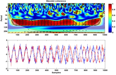
Figure 7: Simple wavelet coherogram of two synthetic signals with growing phase

As aforementioned, wavelet cross-spectrum and wavelet coherence are complex and can be expressed in terms of absolute value and phase. As argued in Grinsted et al., 2004, an useful way to see the phase evolution in time-scale space is the overlay plotting of the phase angle on the cohe-rogram (figure 7). The relative phase relationship can be plotted using arrows with in-phase plotting right, anti-phase plotting left and 90° pointing straight down while the 5% significance level against red noise is shown as a thick contour. In figure 8 an example of wavelet coherence is shown (Cannata et al., 2010). In particular, the relationship between amplitude of continuous background seismic signal (figure 8a) and soil CO2 flux (figure 8b) both recorded at Mt. Etna during the period 2003-2005, was investigated using cross-wavelet spectrum (figure 8c) and wavelet coherence (figure 8d). As explained before, the vectors indicate the phase difference between CO2 flux and tremor amplitude time series. Horizontal arrow pointing from left to right signifies in phase and an ar-row pointing vertically upward means the first series lags the second one by 90°. The 5% significance level against red noise is shown as a thick contour and the COI, where the edge effects might distort the picture (see section 2.1.2), is shown as a lighter shade.

Figure 8: a) tremor amplitude; b) CO2 flux; C) cross-wavelet spectrum and d)

wavelet coherence between the time series in a) and b) (both time series were standardize before cross-wavelet spectrum and wallet coherence computation). The 5% significance level against red noise is shown as a thick contour. The black dashed lines indicate the onset and the end of the eruption.