MICROFLUIDIC CHIP: EXPERIMENTAL RESULTS
In this chapter, all the required operations to fabricate the microfluidic chip, as well as the steps to characterize it, are described. The validation of the PDMS chip is reported, demonstrating the possibility to perform in vitro cell studies for more then 5 hours. In addition, the surface modification of the substrate with patterns of proteins was achieved, and evidence of cellular localization and immobilization are presented.
4.1 MICROFLUIDIC CHIP FABRICATION
The chip fabrication starts with the creation of the PDMS layers: the top and the bottom layer. The layers are created using soft lithography. The mold for the top layer is obtained from patterning a negative photoresist. SU8-10 is poured on a silicon wafer, previously cleaned with sequential washes of acetone, ethanol, and isopropanol and then dried with nitrogen gas. The photoresist is spun at 3500 rpm for 30 s to obtain a thickness of about 10 μm. The wafer is then heated through a soft bake temperature cycle to remove solvent (2 min at 65 °C, 4 min at 95 °C, 2 min at 65 °C) and exposed for 30 s with collimated UV light. After exposure, the wafer is baked through a post bake cycle (1 min at 65 °C, 2 min at 95 °C, 1 min at 65 °C) to amplify the photopolymerization of the resist. It is then developed for 15 s with SU-8 developer and rinsed with isopropanol. Finally, a hard bake is performed consisting of heating the wafer for 1 or 2 h at 150 °C. The wafer is then inspected under a microscope (figure 4.1).
Figure 4. 1 Negative photoresist patterned on a silicon wafer.
The mold for the bottom layer is created with positive photolithography. Photoresist S1813 (Shipley) is used to create channels having a height of 2.5 μm. It is important that the fluidic channels are low to enable the control channels to close them at the lowest possible pressure. However, the height of the fluidic channel should never be lower then 1/10 of its width to avoid collapsing the channel. The S1813 is poured on a clean silicon wafer and spun at 1000 rpm for 1 min. It is prebaked for 1 min at 110 °C, exposed for 30 s with collimated UV light, developed with MF319 developer for approximately 1 min, and rinsed with DI water. The positive photoresist finally requires heating at 125 °C for 25 min in order to allow for the reflow of the polymer, thus, forming a bell shaped cross section of the channel. Figure 4.2 depicts the mold used for the chip’s bottom layer.
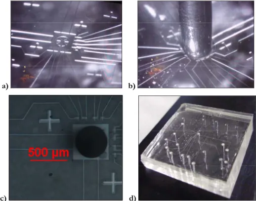
Chip realization continues with the replication of the two molds using PDMS (Sylgard 184 kit, Dow Corning) soft lithography. The first step of this process requires mold silanization. The two wafers are put in a box containing a Petri dish filled with a small amount (a few drops) of trimethylchlorosilane (TMCS) (Sigma-Aldrich). The box is then closed, TMCS can thus evaporate and molecules react with the mold surfaces, forming an anti-sticking layer. This layer facilitates the peeling operation required to separate the molds from the PDMS stamps. The PDMS, used to realize the fluidic channels (the bottom layer in this case), is prepared with a monomer to catalyst ratio equal to 20:1. 10 g of monomer are used, and the two components are then mixed for few minutes and put into a vacuum chamber to rapidly remove the air bubbles formed during mixing. When all the bubbles of air are removed from the PDMS, it is poured on the silicon mold, spun at 6000 rpm for 3 min, and then left to relax for 30 min. The PDMS used to realize the control channels is prepared with a monomer to catalyst ratio equal to 5:1. 25 g of monomer are used, and the two component are mixed for a few minutes, poured directly on the negative mold (which is contained in a Petri dish previously covered with aluminium foil), and then put into the vacuum chamber for air removing. After 30 minutes, the two wafers are put into the oven at 80 °C for 18 min. After that time, the polymerization has not yet been completed, but the polymer is cured enough to be manipulated. In fact at this point of the process, the control layer is first removed from the silicon mold, and the control inlet inputs are created. The holes are realised by a manual hole-punching machine coupled to an illumination system and to a camera interfaced with a monitor where the user can easily view the tip of instrument being brought in proximity to the marked holes on the PDMS (figure 4.3).
a) b) c)
Figure 4. 3 a) Punching set up; b) punching needle; c) punching operation.
The punched control layer (figure 4.4) is then aligned to the fluidic one.
Figure 4. 4 Control layer.
This procedure is done manually with the samples under a microscope. Figure 4.5 shows the alignment set up and the alignment of the control layer to the fluidic one.
a) b)
Figure 4. 5 a) Alignment set up composed of a microscope interfaced with a monitor; b) a control layer overlapping a fluidic layer on a silicon chip.
The alignment procedure of the two layers is delicate because it determines whether the whole chip, the valves and the channels, will function correctly. The control valves should be exactly positioned on the fluidic layer, and, for this reason, the two layers usually have reference marks that indicate the quality of the alignment that is being performed. Some consequences of bad alignment include: channels of the control layer laying the fluidic ones as figure 4.6 a shows or valves that do not cross the fluidic channels as figure 4.6 b depicts.
a) b)
Figure 4. 6 Example of alignment that must be avoided.
After alignment, the chip is put in an oven at 80 °C for 3 h to complete the polymerization and bond the two layers together. Afterwards, the chip is removed from the positive wafer with a scalpel (figure 4.7).
Figure 4. 7 Sequence of operations for removal from the silicon wafer.
Fluidic and cell inlets are then realised as previously described for the control layer, being careful to use a different tip with a smaller diameter for
the cell inlet realization. Figures 4.8 a and b show the cell inlet realization, and figures 4.8 c and d show a photograph of the chip state at this point of the process.
a) b)
c) d)
Figure 4. 8 a) and b) cell inlet hole creation, c) high- and d) low-magnification photo of the final microfluidic chip.
At the end of the procedure, it is possible to reuse the molds. PDMS remaining on the control-channels mold is removed manually paying attention not to break the wafer, while the thin layer of PDMS on the fluidic-channel mold is removed by pouring new PDMS, then removing it by peeling after polymerization.
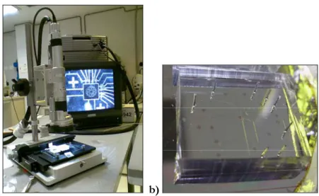
When the chip is ready, it is put on a cover glass and the functionality of the valves is tested. This procedure consists in pushing air into the control inlet with a syringe observing the chip with an inverted microscope: if the valves work properly, the closing of the fluidic channels is easily visible (figure 4.9).
Figure 4. 9 Preliminary valve testing at different gradual air injections.
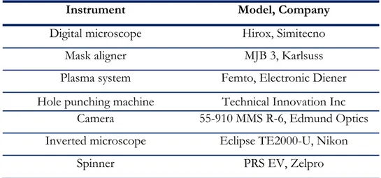
The PDMS chip and the glass slide are bonded together through plasma bonding. The cover glass is processed by two different cycles of plasma oxygen treatment. After 2 min for vacuum creation, a continuous flow of oxygen is inserted into the chamber for 2 min in order to stabilize the pressure, and then the glass slide is exposed for 45 s to plasma (40 kHz at 100 W). Then the chips are put into the same chamber of the plasma oxygen system, and another different cycle is performed: 5 min of vacuum, 5 min for oxygen inlet and 45 s of exposition to plasma (40 kHz at 20 W). Figure 4.10 shows the plasma oxygen system while table 4.1 summarizes the instruments required for chip realization.
Table 4. 1 Instrumentation used during chip realization.
Instrument Model, Company
Digital microscope Hirox, Simitecno
Mask aligner MJB 3, Karlsuss
Plasma system Femto, Electronic Diener
Hole punching machine Technical Innovation Inc
Camera 55-910 MMS R-6, Edmund Optics
Inverted microscope Eclipse TE2000-U, Nikon
Spinner PRS EV, Zelpro
4.2 MICROCHIP TESTING
In order to pneumatically actuate each soft valve, the bulge of the PDMS control channel is ensured by the functioning of a solenoid valve. It uses compressed air to pressurize the fluid in the PDMS control channel. Every control channel is regulated by an own pressure line which is switched on\off through its own pneumatic solenoid valve. Solenoid valves are chosen because they offer fast and safe switching, high reliability, long service life, low control power and compact design. Valves are controlled by custom electronic units connected to a computer. Each valve can be individually controlled through a LabVIEW software interface (NI) which allows the user to set the closing and opening times. Figure 4.11a shows the electronic components of the control system. Focusing on the valves (element 1 in figure 4.11a), note that they all are connected to an air pressurized tube for input (7) and to a channel filled of water as an output (9). These channels are connected to the chip control channels via control tubes (Tygon® R-3603 with a 0.51 mm diameter) as indicated in figure 4.11 b.
a) b)
Figure 4. 11 a) Valve system control: 1) valves, 2) electric control signal board, 3) connector block, 4) cable for the connection to NI DAQCard-DIO-24, 5) rectifier, 6) stabilization direct current circuit, 7) air inlets, 8) voltage transformer, 9) outlet tubes. b) Connections of the outlet tubes with the control tubes.
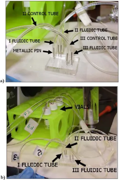
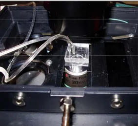
The control tubes are filled with water and then they are connected to the chip control inlets with metallic pins (tube AISI 304, external/internal diameter 0.65/0.35, 12.5 mm length, Unimed) (figure 4.12). When a solenoid valve is opened, the water is pressurized and pushed into a chip control channel causing the closing of the corresponding fluidic valve.
Figure 4. 12 Connection of a control tube with a control channel.
The fluidic channels are also connected to flexible tubes (Tygon® R-3603 Laboratory Tubing) with the same type of metallic pin. The other side of the fluidic tubes are inserted into pressurized vials (National Scientific) containing the substance that should be delivered through the chip channel.
The vial pressure is controlled with a manual pressure regulator. Figure 4.13 a shows the chip with fluidic and control tubes connected through metallic pins. In the described case, the chip uses three fluidic channels connected to three own tubes (precisely indicated as I, II and III). II and III are connected to channels which are controlled by their own valves, while I is not controlled and lets the fluids flow undisturbed. Figure 4.13 b shows the same chip and the vials located in a yellow rack. Some tubes (labelled with “F”) are also visible entering the vials. These tubes are necessary for pressurizing the fluid inside the vials.
a)
b)
Figure 4. 13 a) Connections of a chip that has two active valves controlling their own fluidic channels (II and III) and one channel for continuous fluid inlet (I); b) connections of fluidic tubes to vials pressurized by air injection delivered from tubes named F3, F2 and F1.
After having connected all the necessary tubes, the chip is mounted on the stage of an inverted Nikon TE2000 microscope (Nikon Inc., Japan). The objectives used for the experiments are a 20x (0.45 NA) and a 40x (1.3 NA) (Plan Fluor, Nikon). The microscope also includes an incubation chamber for live-cell experiments (figure 4.14).
Figure 4. 14 Chip with control and fluidic tubes ready for image acquisitions.
Figure 4.15 summarizes the experimental set up system used for all the tests performed.
4.2.1 Valve characterization
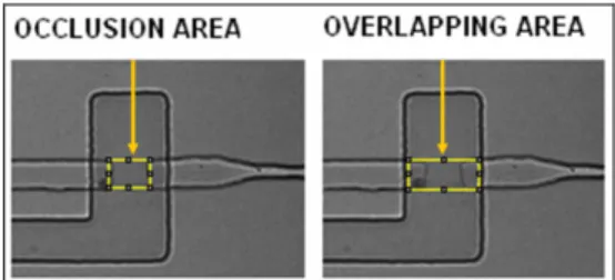
To characterize the functionality of the PDMS valves, some tests were performed. As preliminary test, the minimum pressure value to obtain the occlusion of the fluidic channel was determined. The valve channel was filled with water and pressurised. Photos of the overlapping region between the control and fluidic channels were acquired by a CCD camera (ORCA ER, Hamamatsu) for different values of the pressure applied to the valve. The collected photos were then loaded into ImageJ (National Institute of Health, USA) software. Through some program tools, both the occlusion area and the overlapping area between the fluidic and control channels were calculated. The ratio of these areas was called the occlusion index and it indicates the valve occlusion efficiency (figure 4.16).
Figure 4. 16 Fluidic channel occlusion by the valve.
It was observed that at pressures below 5 psi1 occlusion does not occur but
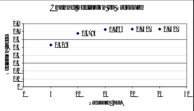
at 5 psi the valve responds readily to the applied pressure resulting in a half occlusion of the fluidic channel. Increasing the pressure of the control channel the occlusion index becomes greater, reaching a saturation value of about 0.7 for pressures greater than 15 psi (figure 4.17).
Channel occlusion vs Pressure 0,5296 0,6794 0,7266 0,7317 0,7317 0 0,1 0,2 0,3 0,4 0,5 0,6 0,7 0,8 0 5 10 15 20 25 30 Pressure (psi) Oc c lus io n I nde x
Figure 4. 17 The occlusion index as a function of the pressure in the control channel.
Despite the bigger occlusion at 20 and 25 psi, at these pressure values the valve shows a delay during opening. Since this behaviour is not visible at 15 psi, this value was chosen for all the experiments. In addition, it was observed that the time response of the valve at 15 psi is quite fast: it was measured that the valve maximum operation frequency is 3 Hz (166 ms of opening and closing), while at 4 Hz it does not open completely owing to the known PDMS hysteresis effect2. Moreover, the valve working
frequency is a parameter that influences the release of fluid volumes.
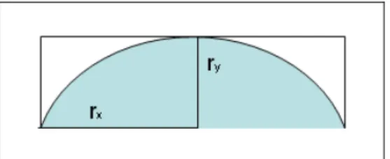
To quantify the fluid delivery, the system was tested at 0.5 Hz (2 seconds of valve opening time) and with a fluidic channel pressurized at 15 psi. First, the velocity of the output fluid near the fluidic channel was calculated. The measurement was obtained observing the motion of the meniscus of culture medium inside the fluidic tube for a defined time period. From the mass conservation principle, it is possible to establish the equivalence between the fluid motion inside the tube and the fluid motion inside the fluidic channel, obtaining that, at the end of fluidic channel, the fluid has a mean velocity of 27 mm/s3. To establish the volumetric rate of
channel, the fluid speed was multiplied by the cross section of the channel,
2As reported in reference [3] of Chapter 2.
which was assumed to be a ellipse with semi-major and minor-axis of 5 μm and 2.5 μm respectively (figure 4.18).
Figure 4. 18 Cross section of the fluidic channel used for determining the fluid delivery speed.
Under these conditions the system delivers 1.8 μl/h of fluid.
4.2.2 Concentration gradient characterization
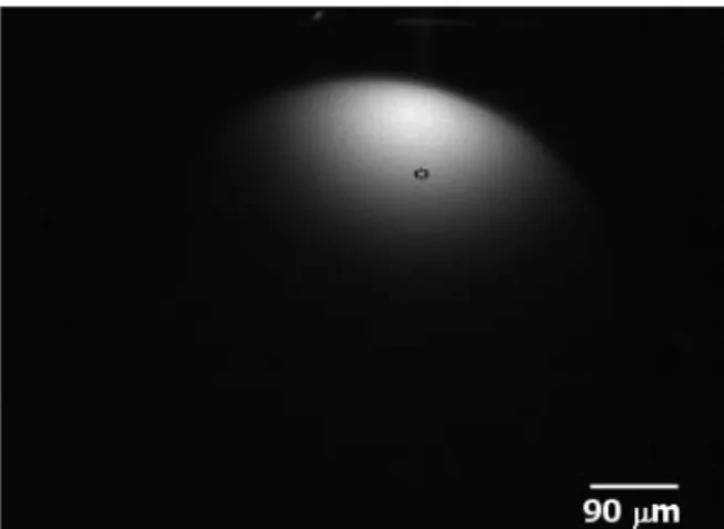
The system validation consisted in some experiments showing first one channel functioning, then the contemporary functioning of two orthogonal channels. To observe the concentration gradient, a fluorescein isothiocyanate solution (Sigma-Aldrich, Catalogue number F7250), a fluorophore commonly used in microscopy that has an absorption maximum at 494 nm and emission maximum of 521 nm (in water), was used. The light signal intensity revealed by a camera was associated to the fluorescein concentration. All the experiments started with the filling of the chamber with water, to make fluorescein diffusion possible. Water continuously entered through one of the fluidic channels, which was pressurized at 15 psi during the whole experiment. First tests examined the concentration gradient generated by a single channel at different fluidic pressures: 5, 10 and 15 psi (figure 4.19).
Figure 4. 19 Bright field photo of a chip showing the summary of gradient generation experiments with a single channel at different fluidic channel pressures.
The system separately controls each valve, and the user sets the opening and closing times as desired. In this case the valve frequency is 0.25 Hz (50 % duty cycle), swollen by 15 psi pressure (figure 4.20)
Figure 4. 20 Control signal applied to the solenoid valve.
Photos were taken every 300 ms for 3 min and they were analysed by ImageJ. This software has a simple tool that can be used for calculating the mean intensity value of a user-defined area of a selected image. The chosen area is circular with a mean pixel number equal to 200 (figure 4.21).
Figure 4. 21 Frame showing the circular area where the mean intensity value is calculated.
For that area the fluorescence intensity signal over time was calculated. Figure 4.22 presents some several concentration profiles obtained during this experiment.
Figure 4. 22 Fluorescence signal at different times and for different pressures.
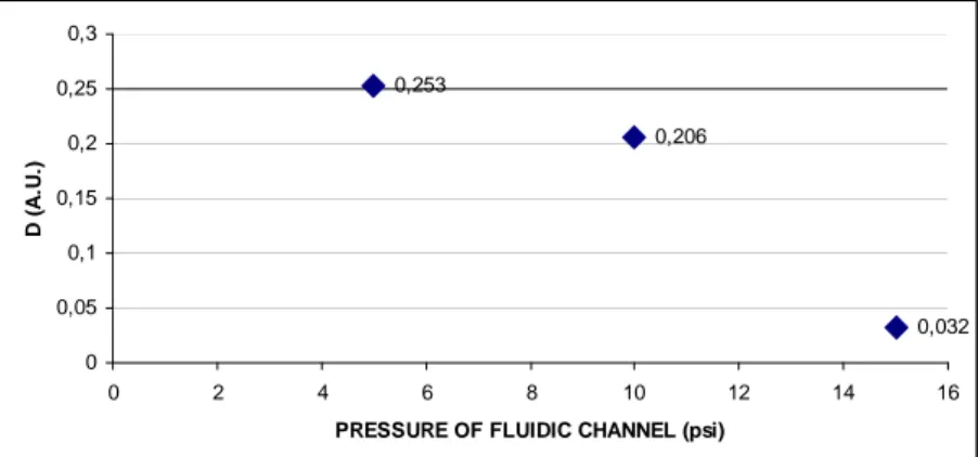
Every frame has the fluorescence intensity signal normalized to the white value (which represents the highest signal). As shown in figure 4.23, after the transient period, the curves show a cyclic trend with different mean values related to the different pressures which regulate the volumetric rate of fluorescent solution. In this cyclic trend every curve shows a minimum
and a maximum value. It is observed that the difference between these values, D, decreases with the increasing of the pressure value (figure 4.24).
Figure 4. 23 Fluorescence intensity as a function of time at different pressures.
0,253 0,206 0,032 0 0,05 0,1 0,15 0,2 0,25 0,3 0 2 4 6 8 10 12 14 1
PRESSURE OF FLUIDIC CHANNEL (psi)
D (A
.U
.)
6
Figure 4. 24 D values as a function of the pressure applied to the fluidic channel.
To characterize the florescence intensity profile along the fluidic channel direction, other measurements were taken at 150, 200, 250, 300 and 350 μm from the outlet channel. The 2D fluorescence intensity profiles, resulted from plotting the mean fluorescence intensity values at different distances from the fluidic channel, are shown in figure 4.25.
0,00 0,10 0,20 0,30 0,40 0,50 0,60 0,70 0,80 0,90 100 150 200 250 300 350
DISTANCE FROM SOURCE (um)
NO RM AL IZ E D M E AN INT E NS IT Y ( A. U. ) 5 psi 10 psi 15 psi
Figure 4. 25 Fluorescence intensity profiles at different pressures over distance from the source (for t > 50s).
The experimental values were then fitted in order to have an analytical expression for the concentration profile. The curve fitting tool of MATLAB (MathWorks) was used. A simple exponential decay was used for fitting x b e a x f( )= ⋅ − ⋅
where a is the intensity value at x equal to 0 and b represents the characteristic length which expresses the distance from the source at which the fluorescence intensity is reduced to the 30% of initial value. Figure 4.26 shows the fitted curves at different pressures.
Figure 4. 26 Fluorescence intensity profile along the fluidic channel direction at different pressures.
After fitting data, the program returns the goodness of fit statistics, like the R-square which represents the square of the correlation between the response values and the predicted response values. R-square is defined as the ratio of the sum of squares of the regression (SSR) and the total sum of squares (SST). SSR is defined as 2 1 ) ˆ (
∑
= − = n i i i y y w SSRSST is also called the sum of squares about the mean, and is defined as
2 1 ) (
∑
= − = n i i i y y w SSTwi are the parameters calculated by the software. R-square can take on any value between 0 and 1, with a value closer to 1 indicating a better fit. For example, an R2 value of 0.998 means that the fit explains 99.9 % of the total
variation in the data about the average. Table 4.2 summarizes the a, b and R2 values obtained for the fitting of the fluorescence intensity profiles.
Table 4. 2 Fitting parameters and goodness of fit statistic.
A 1/b (μm) R2 5 psi 1.133 117.6 0.998 10 psi 1.099 123.1 0.996 15 psi 1.985 117.3 0.995
In order to demonstrate the versatile use that this system can offer, the gradient generated by two orthogonal channels is shown. The valve
opening/closing sequence is the same for both channels (figure 4.27) but they are not opened at the same time.
Figure 4. 27 Control signals applied to the control valves: left valve (first row) and up valve (second row).
The experiment performed is depicted in figure 4.28.
Figure 4. 28 Gradient generation experiment with two orthogonal channels at 10 psi channel pressure.
Figure 4.29 shows the concentration profile at 14 s after the left channel opening.
Figure 4. 29 Frame showing the circular area where the mean intensity value is calculated.
Figure 4.30 shows the concentration profile at different times while figure 4.31 presents the fluorescence intensity signal revealed at 100 μm from the upper outlet (see also Fig. 4.29).
Figure 4. 31 Fluorescence intensity as a function of time at 10 psi.
To observe the florescence intensity profile along the fluidic channel direction, other measurements were performed at 150, 200, 250, 270, 300 and 350 μm distances from the outlet (figure 4.32).
10 psi 2 ORTHOGONAL CHANNELS
0,59 0,35 0,22 0,15 0,14 0,08 0,06 0 0,1 0,2 0,3 0,4 0,5 0,6 0,7 100 150 200 250 270 300 350
DISTANCE FROM SOURCE (um)
N O R M A L IZ E D M E A N IN T E N S IT Y ( A .U .) 10 psi 2 ORTHOGONAL CHANNELS
Figure 4. 32 Fluorescence intensity data over the distance from injection point.
Figure 4.33 depicts the 2D fluorescence intensity data of the orthogonal channels compared with the single channel 10 psi test, previously
performed (figure 4.25 b). Near the upper channel, the trends are quite similar, but, arriving at 250 μm, the composition of the superimposing flows is evident. 0 0,1 0,2 0,3 0,4 0,5 0,6 0,7 100 150 200 250 270 300 350
DISTANCE FROM SOURCE (um)
NO RM A L IZ E D M E AN I NT E NS IT Y ( A. U. ) 10 psi 2 ORTHOGONAL CHANNELS
10 psi SINGLE CHANNEL
Figure 4. 33 Fluorescence intensity profile of two orthogonal channels, (pressurized at 10 psi), along fluidic channel direction compared to the only channel profile.
To observe the concentration gradient trend, the curves were derived. The curve derivate fitting tool of MATLAB (MathWorks) was used. It chose some points of the interpolated experimental data to establish the change in y and the change in x, then it calculated the slope. For the single channel it was observed that increasing the distance from source, the gradient progress gradually reaches the zero value, but, as expected, the presence of an orthogonal delivering channel modifies its trend (figure 4.34 a and b).
a) 0 0.1 0.2 0.3 0.4 0.5 0.6 0.7 N O R M A LI Z E D M EAN IN T E N S IT Y (A .U .)
DISTANCE FROM SOURCE (um)
10 psi SINGLE CHANNEL
100 150 200 250 300 350 -5 -4 -3 -2 -1 0x 10 -3 1s t d er iv b) 0 0.1 0.2 0.3 0.4 0.5 0.6 0.7 N O R M A LIZ ED M E A N IN T E N S IT Y ( A .U .)
DISTANCE FROM SOURCE (um)
10 psi 2 ORTHOGONAL CHANNELS
100 150 200 250 300 350 -6 -5 -4 -3 -2 -1 0x 10 -3 1s t de riv
Figure 4. 34 a) Normalised mean intensity data of the experiment with a single working channel. The program automatically calculates a curve, which interpolates the experimental results, and then it calculates the first derivate on the interpolated curve; b) normalised mean intensity of experimental data (in two orthogonal working channels experiment) and the first derivate of the interpolated curve.
4.3 CELL VIABILITY TEST
To demonstrate the ability of the developed system to sustain experiments with cells, some tests were performed. In particular, staining viable cells, it was possible to evaluate the optimal average value of cells density and the maximum time for experiments without altering the viability of the cells. With this aim, cells nuclei were stained with a fluorescent dye, and maintained overnight without renewal of fresh medium inside the microfluidic chip.
The experiments started with cell suspension preparation and its loading. Following the protocols described in Chapter 3 section 3.3, REFs were tripsinized, centrifuged, counted and suspended in 1 ml with a final concentration of 5 x 10⁵ cells/ml. Cells were suspended in fresh cell culture
medium, containing 10 % of Hoechst dye (0.1 g/l) (33342, Sigma). The Hoechst (2(4-hydroxyphenyl)-5{5-(4-methylpiperazine-1-yl)-benzimidazol-2-yl}benzimidazole) is a type of bis-benzimidazole dye that binds to DNA. It is commonly used in the laboratory to analyze and quantify DNA in live or fixed cells and for separate viable cells from apoptotic cells. Hoechst 33342 is a lipophilic structure that can cross the cell’s lipid membranes and reach the DNA. It has an maximum absorption at 360 nm and maximum emission of 485 nm. The cell suspension was loaded in a syringe (1 ml): after connecting the syringe tip to the cell input port, the suspension was injected into the microfluidic chamber using a manual pressure (figure 4.35). The operation was carried on under an optical microscope in order to fill the cell culture volume.
a) b)
Figure 4. 35 a) Cell loading and b) a particular of cell input port.
Cells do not appear damaged by the injection procedure: any lysed or apoptotic cells can be found in the fluorescence image (figure 4.36), where the stained nuclei appear clearly defined. The cell density in the chamber, starting from a solution of 5 x 10⁵ cells ml-1, is around 300 cells mm-2.
Figure 4. 36 Fluorescent image of the chip: blue stained nuclei are clearly visible.
To monitor the cell vitality inside the chip a time lapse microscopy experiment was run. The chip was mounted in the thermostatic chamber (previously mentioned in section 4.2) and observed with a 20x objective. The cell imaging was performed for five hours and photos of the stained nuclei were taken, every five minutes, using a digital camera (ORCA ER, Hamamatsu) (figure 4.37).
Figure 4. 37 Fluorescence microscopy of cells in the chip chamber, at the start of experiment, with a zoom of a cellular nucleus.
This test provides a preliminary evaluation of the compatibility of the PDMS chip: cells are maintained viable for at least five hours, suggesting that, renewing the culture medium, the microsystem can be useful for future long term studies and cell analysis. Furthermore, the selected cell density (300 cells mm-2) represents an optimal starting value for seeding
cells, in particular for short term experiments and analysis (up to 12 h).
4.4 MICROPATTERNED SUBSTRATE
As previously stated (Chapter 3, section 3.1.3), micropatterning was achieved by casting PDMS on a master obtained by a photolithography process. The template for the PDMS is a negative photoresist pattern on a silicon wafer spun at 6000 rpm for 30 s, then exposed with collimated UV light for 30 s and developed in SU8 developer for 2 min. After a 1 h hard bake at 150 °C the mold is ready (figure 4.38).
a) b)
c)
Figure 4. 38 a), b), c) Silicon wafer (white) and photoresist layer (grey).
To prepare the PDMS stamp, 20 g of liquid prepolymer of PDMS with a monomer to catalyst ratio equal to 10:1 is poured over the template pattern and cured at 100 °C for 1 h. The surface of the template substrate is previously treated with TCMS for the ease of removing the cured stamp (see Cap. 4, Sec. 4.1 ). The resulting PDMS stamp (5 mm of thickness) is cut into 0.25 cm2 pieces (figure 4.39).
Figure 4. 39 PDMS stamp.Micropatterned areas are present on the bottom of the stamp.
PDMS stamps are then sonicated for 5 min in ethanol, rinsed with ethanol, blown dry with a nitrogen flux and left in the flow hood for at least 1 h to evaporate the residual ethanol. Then they are inked with a fibronectin
solution (Fibronectin from Human plasma, Sigma) 50 μg/ml each in H2O.
The resulting FN-inked stamps are incubated for 45 min at room temperature. After this time has elapsed, the protein solution is removed with a pipette until the stamp surface looks completely dry. The stamps are immediately placed in contact with a 35 mm glass bottom dish (Will-Co-Dish GWSt-3522) and they are pressed slightly with tweezers for several seconds to guarantee conformal contact. After 5 min the stamps are removed, the substrate is washed once with water and incubated in 10 mM HEPES, ph 7.4, containing 0.1 mg/ml PLL-g-PEG (SurfaceSolutionS, Switzerland) for 1 h. The substrate is then rinsed twice with PBS and used for experiments. Figure 4.40 shows a cover glass with fibronectin pattern (dark stripes) and passivated with PLL-g-PEG labelled with rhodamin (red). The stamps are cleaned for one hour in water and reused several times.
Figure 4. 40 Glass substrate passivated with rhodamin labelled PLL-g-PEG.
To observe the correct fibronectin transfer to the substrate, the protein is labelled with AlexaFluor488 using an antibody labelling kit (Molecular Probes). It requires the use of an anti-human fibronectin solution (Sigma) and the incubation with the Zenon labelling reagent, containing a fluorophore-labeled “Fab” fragment which binds to the “Fc” portion of the antibody. When the fibronectin labelling is ready, the protein is incubated on the PDMS stamp in the dark for 45 min. The protein pattern is observed with a fluorescence microscope, using a 20x objective (figure 4.41).
Figure 4. 41 Fibronectin patterns transferred onto a glass Petri dish.
4.5 CELL ADHESION ON FIBRONECTIN
To characterize the cell adhesion properties on the micropatterned substrates, two different cell types were used: REFs and SH-SY5Y. REFs were plated on the fibronectin patterns (created as previously described) at a density of 8000 cells cm-2. The density was chosen considering that inside
the chamber at least a minimum group of 10-20 cells number of cells can be seeded. After only 3 hours of incubation, it was observed that cells internalize the PLL-g-PEG, but it was not found if this could damage cells in any way. After 24 hours, a selective adhesion on the stripe of fibronectin areas was observed. Figure 4.42 a shows the adhesion of a REF on the FN pattern and a round cell in correspondence with the passivated area. REFs express a dyed paxillin, which is a cytoskeletal component of focal adhesions4. Figure 4.42 b also presents the paxillin distribution inside the
cell.
a) b) Figure 4. 42 a) Stripes of Fn pattern and REF adhesion. The figure shows the PLL-g-PEG internalization. The contrast and the brightness of image are modified in order to highlight the pattern geometry. b) REF paxillin distribution.
The day after the seeding, not-spread and floating cells were removed by extensively washing the surface with PBS and it was observed that it did not cause cell detachment. Figure 4.43 shows a cell cluster after washing. The tendency of cells to spread over fibronectin pattern is confirmed: several filopodia are visible, which are cytoskeletal actin projections on the mobile edge of the cell and are involved in the cellular adhesion mechanism.
b)
c)
d)
Figure 4. 43 a) and c) show the adhesion of cells on Fn patterns and the passivated areas, probably cell bodies are detached from the passivated substrate confirming the efficacy of passivation. The contrast and brightness of images were modified to highlight the pattern geometry. b) and d) represent cells on Fn pattern.
At the third day of culture, the washing caused definitive cellular detachment.
The experiments performed with SH-SY5Y cells also confirmed the selective adhesion on the micropatterned areas. In order to observe a larger number of cells, they were plated at 80000 cells cm-2 density. Three days
after seeding, the pattern remains stable and a lot of cells adhered on the substrate with fibronectin patterns, forming clusters of rounded cells (figure 4.44 a). After extensive washing with PBS, many cells remained adherent on the fibronectin patterns (figure 4.44 b).
a) b)
Figure 4. 44 a) Cell adhesion three days after the seeding; b) cell adhesion after washing.
Even if these tests required further accurate statistical analysis, in order to have a precise quantification of cellular adhesion, they are useful in confirming the functionality of the method; in particular, for SH-SY5Y cells, experimental results of cell guidance can not be found in literature. For both REF and SH-SY5Y cells, the stripe pattern appears to be unable to provide the adhesion of the whole cell body. For this reason, future studies will require the design of 20 μm wide stripes.