Chapter 4
Centaurs and TNOs
As already stated, Trans-Neptunian Objects and Centaurs are the most pris-tine remnants of the proto-planetary disk in which the accretion of the plan-etesimals occurred. Hence, their study is fundamental in the understanding of the conditions existing in the early Solar System, and of the accretion processes which governed the planetary formation at large heliocentric dis-tances.
In October 2006, a two-year Large Programme started at ESO to study these bodies. During 500 hours of observation, data on 50 objects have been obtained using different techniques (spectroscopy, photometry, polarimetry).
As part of my PhD work, I contributed to the ESO-LP with:
• Spectroscopy and modelling: I carried out two observing runs (1 night each) at the VLT, acquiring 8 visible and 3 J-band spectra with the instruments FORS2 and ISAAC, respectively. I reduced most part of the ISAAC spectroscopic data obtained within the ESO-LP, and I contributed to the analysis and interpretation of the spectra.
• Colors and taxonomy: During the above-mentioned observing runs with FORS2 and ISAAC, I also acquired visible (8 objects, V RI filters)
and NIR (6 objects, JHKs filters) photometric data. I reduced most
part of the NIR photometric data obtained in the framework of the ESO-LP, and I took in charge the analysis and interpretation of the whole V-NIR photometric dataset.
• Light curves and densities: I carried out two observing runs (3 nights each) at the NTT, acquiring the light curves of 12 Centaurs and TNOs with the EMMI instrument. I took in charge the reduction, the analysis, and the interpretation of the whole dataset.
4.1
Spectroscopy and modelling
As stated in section 1.2.2, the spectroscopic technique provides the most detailed information on the compositions of TNOs. In the visible and NIR spectral ranges, diagnostic features of silicate minerals, feldspar, carbona-ceous assemblages, organics, and water-bearing minerals are present. Signa-tures of water ice are present at 1.5, 1.65, 2.0 µm, and signaSigna-tures of other
ices include those due to CH4 around 1.7 and 2.3 µm, CH3OH at 2.27 µm,
and NH3 at 2 and 2.25 µm, as well as solid C-N bearing material at 2.2 µm.
4.1.1
Observations and data reduction
During the ESO-LP, visible and NIR spectroscopy has been performed at the ESO-VLT (Paranal, Chile) within several runs between October 2006 and November 2008.
Low resolution (∼ 200) visible spectroscopy was performed with the two FORS (FOcal Reducer and low dispersion Spectrograph) instruments (FORS1 until September 2007, FORS2 later on), and the obtained data were reduced according to the procedures described in section 2.2.1.
J-band (1.1-1.4 µm) spectroscopy was performed using ISAAC (Infrared Spectrometer And Array Camera) with a spectral resolution of about 500, while the H + K grating of SINFONI (Spectrograph for INtegral Field Ob-servations in the Near Infrared) was used to yield a spectral resolution of about 1500 over the 1.45-2.45 µm range. NIR spectra have been reduced as explained in section 2.2.2; each of them has been smoothed with a median filter technique to increase the signal-to-noise ratio, yielding a final resolution of 100-250 for both ISAAC and SINFONI data.
To combine visible and NIR spectra, photometric data are used. First, visible spectra are normalized at the V filter wavelength. Then the NIR
spectra are scaled to the J, H, Ks magnitudes, transformed in reflectance
using the following relation:
Rλ = 10−0.4[(Mλ−V )−(Mλ−V )⊙] (4.1)
where (Mλ − V ) and (Mλ − V )⊙ are the colors of the object and the Sun,
respectively (λ is the central wavelength of the filter used to measure Mλ).
4.1.2
Visible spectra: features and slopes
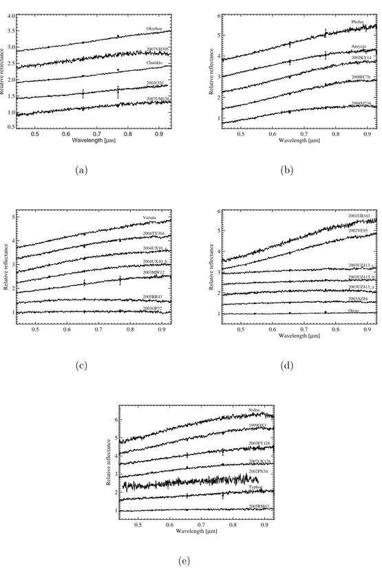
Thirty-one spectra (Fig. 4.1) have been obtained for 28 bodies (6 classical, 5 resonant, 5 scattered and 2 detached TNOs, and 10 Centaurs), 15 of which were spectroscopically observed for the first time ever (Fornasier et al. 2009).
4.1. SPECTROSCOPY AND MODELLING 59 0.5 0.6 0.7 0.8 0.9 Wavelength [µm] 0.5 1.0 1.5 2.0 2.5 3.0 3.5 4.0 Relative reflectance 2007UM126 2003CO1 Chariklo 2007VH305 Okyrhoe (a) 0.5 0.6 0.7 0.8 0.9 Wavelength [µm] 1 2 3 4 5 6 Relative reflectance 2008SJ236 2008FC76 2002KY14 Amycus Pholus (b) 0.5 0.6 0.7 0.8 0.9 1 2 3 4 5 Relative reflectance 2003OP32 2005RR43 2003MW12 2004UX10_b 2004UX10_a 2004TY364 Varuna (c) 0.5 0.6 0.7 0.8 0.9 Wavelength [µm] 1 2 3 4 5 6 Relative reflectance Orcus 2003AZ84 2003UZ413_a 2003UZ413_b 2003UZ413_c 2002VE95 2001UR163 (d) 0.5 0.6 0.7 0.8 0.9 Wavelength [µm] 1 2 3 4 5 6 Relative reflectance 2005RM43 Typhon 2002PN34 2007UK126 2003FY128 1999OX3 Sedna (e)
Figure 4.1 – Visible spectra of Centaurs (a and b), classical TNOs (c), reso-nant TNOs (d), and scattered and detached TNOs (e). Spectra are shifted for clarity. Color indices converted to spectral reflectance are also shown on each spectrum. From Fornasier et al. (2009).
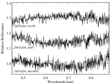
The spectrum of the resonant TNO (208996) 2003 AZ84, acquired in
November 2008, appears featureless, while a weak band attributed to the presence of hydrated silicates, centered around 0.7 µm with a depth of about 3% and a width of more than 0.3 µm, was seen both on a spectrum ac-quired in January 2007 (Alvarez-Candal et al. 2008) and in a previous work by Fornasier et al. (2004). The three spectra after the continuum removal are plotted in Fig. 4.2: the November 2008 data do not show any absorption band, except for some residuals of the background removal (in particular the
O2 band around 0.76 µm and the water telluric bands around 0.72 µm and
0.83 µm). It is hence possible that 2003 AZ84 has an heterogeneous surface
composition.
Also all of the other objects have featureless spectra, with the exceptions of (10199) Chariklo and (42355) Typhon, which show faint absorptions at 0.62-0.65 µm attributed to the presence of phyllosilicates (aqueously altered material) on their surfaces.
0.5 0.6 0.7 0.8 Wavelength [µm] 1.0 1.1 1.2 1.3 1.4 Relative Reflectance 2003AZ84_March03 2003AZ84_Jan07 2003AZ84_Nov08
Figure 4.2 – Visible spectra of 2003 AZ84 taken during 3 different observing
runs, after continuum slope removal. No indication of the band seen in the March 2003 and January 2007 data appears in the spectrum obtained on November 2008. From Fornasier et al. (2009).
Within the obtained results, the large variety in the spectral behaviour of both the Centaur and TNO populations emerged, since the spectral slopes
span a wide range of colors, from gray to very red (∼ 1 to 51 % / 103 ˚A).
For a better analysis of the visible spectral slope distribution, all the mea-surements available in the literature have been taken into account (Fornasier
4.1. SPECTROSCOPY AND MODELLING 61 et al. 2009, and references therein), for a total sample of 20 Centaurs and 53 TNOs (14 resonants, 29 classicals, 6 scattered, and 4 detached objects).
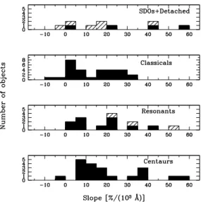
Resonant, scattered and detached TNOs, as well as Centaurs, have very similar spectral slopes, while it is evident that there is a lack of very red objects in the investigated classical TNOs (Fig. 4.3 and Table 4.1). Never-theless, this lack could be due to an observational bias, since the red objects belong principally to the cold population, which presents smaller sizes than the bluer hot population (see section 1.1).
The bimodal distribution (Pholus-like and Chiron-like) suggested for Cen-taurs based on visible photometric colors (see section 1.1), does not clearly appear in the obtained spectral slope distribution, probably because of the limited dataset.
Figure 4.3 – Distribution of TNOs and Centaurs as a function of the spectral slope. From Fornasier et al. (2009).
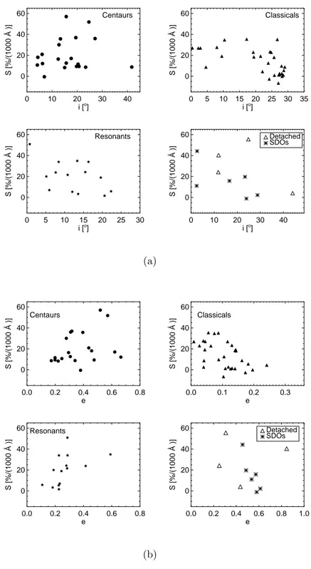
Possible correlations have been searched between spectral slope values (S) and orbital elements (inclination i, eccentricity e, semimajor axis a, and perihelion q) or absolute magnitude H for the different dynamical classes (Fig. 4.4), computing the Spearman’s (1904) rank correlation coefficient (ρ)
and the two-sided significance (Pr) of its deviation from zero. The
Spear-man correlation coefficient is defined as the Pearson correlation coefficient between the ranked (i.e., magnitude-sorted) variables. The Pearson correla-tion coefficient between two variables is, in turn, defined as the covariance of the two variables divided by the product of their standard deviations. Hence:
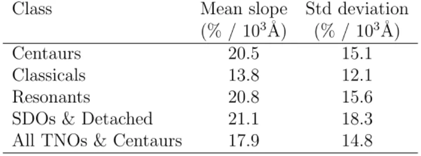
Table 4.1 – Mean spectral slope values and standand deviation of TNOs and Centaurs.
Class Mean slope Std deviation
(% / 103˚A) (% / 103˚A)
Centaurs 20.5 15.1
Classicals 13.8 12.1
Resonants 20.8 15.6
SDOs & Detached 21.1 18.3
All TNOs & Centaurs 17.9 14.8
ρ =
Pn
i=1(xi− ¯x)(yi− ¯y)
q
Pn
i=1(xi − ¯x)2 Pni=1(yi− ¯y)2
(4.2)
where xi and yi represent the magnitude-based ranks among slope and the
other quantity, respectively. Elements of identical magnitude are ranked us-ing a rank equal to the mean of the ranks that would otherwise be assigned. The value of ρ varies between -1 and 1: if it is close to zero this means no correlation, if |ρ| is close to 1 then a correlation exists. To test whether an ob-served value of ρ is significantly different from zero, it is possible to calculate the probability that it would be greater than or equal to the observed value, given the null hypothesis, by using a permutation test. The significance is
hence a value in the interval 0 < Pr < 1, and a small value indicates a
signif-icant correlation. Correlations with |ρ| > 0.5 and Pr < 0.02 are considered
particularly important. The results are summarized in Table 4.2.
Classical TNOs present an anticorrelation between S and i, with lower slope values with increasing inclination (as expected, because of the men-tioned cold and hot populations, see section 1.1) is found. Nevertheless,
considering only the 7 objects with i < 10.4◦, there is no correlation between
S and i (ρ = 0.198206 and Pr = 0.993299), in agreement with the result
by Peixinho et al. (2008), who found that the optical colors of classical
ob-jects are independent of inclination below i ∼ 12◦. A weaker anticorrelation
between S and e is also found for classical TNOs.
Resonant TNOs present a correlation between S and e, with high-e objects redder than those with low eccentricities. Excluding the 3
“non-plutinos” objects, the correlation becomes weaker (ρ = 0.681818 and Pr =
4.1. SPECTROSCOPY AND MODELLING 63 0 10 20 30 40 i [o ] 0 20 40 60 S [%/(1000 Å )] Centaurs 0 5 10 15 20 25 30 35 i [o ] 0 20 40 60 S [%/(1000 Å )] Classicals 0 5 10 15 20 25 30 i [o ] 0 20 40 60 S [%/(1000 Å )] Resonants 0 10 20 30 40 i [o ] 0 20 40 60 S [%/(1000 Å )] Detached SDOs (a) 0.0 0.2 0.4 0.6 0.8 e 0 20 40 60 S [%/(1000 Å )] Centaurs 0.0 0.1 0.2 0.3 e 0 20 40 60 S [%/(1000 Å )] Classicals 0.0 0.2 0.4 0.6 0.8 e 0 20 40 60 S [%/(1000 Å )] Resonants 0.0 0.2 0.4 0.6 0.8 1.0 e 0 20 40 60 S [%/(1000 Å )] Detached SDOs (b)
Figure 4.4 – (a) Spectral slope versus orbital inclination for Centaurs and TNOs. (b) Spectral slope versus orbital eccentricity for Centaurs and TNOs. From Fornasier et al. (2009).
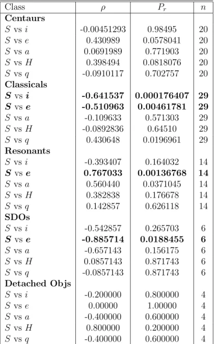
Table 4.2 – Computed Spearman correlations between spectral slope and orbital elements (i, e, a, q) or absolute magnitude H of Centaurs and TNOs. From Fornasier et al. (2009).
Class ρ Pr n Centaurs S vs i -0.00451293 0.98495 20 S vs e 0.430989 0.0578041 20 S vs a 0.0691989 0.771903 20 S vs H 0.398494 0.0818076 20 S vs q -0.0910117 0.702757 20 Classicals S vs i -0.641537 0.000176407 29 S vs e -0.510963 0.00461781 29 S vs a -0.109633 0.571303 29 S vs H -0.0892836 0.64510 29 S vs q 0.430648 0.0196961 29 Resonants S vs i -0.393407 0.164032 14 S vs e 0.767033 0.00136768 14 S vs a 0.560440 0.0371045 14 S vs H 0.382838 0.176678 14 S vs q 0.142857 0.626118 14 SDOs S vs i -0.542857 0.265703 6 S vs e -0.885714 0.0188455 6 S vs a -0.657143 0.156175 6 S vs H 0.0857143 0.871743 6 S vs q -0.0857143 0.871743 6 Detached Objs S vs i -0.200000 0.800000 4 S vs e 0.00000 1.00000 4 S vs a -0.400000 0.600000 4 S vs H 0.800000 0.200000 4 S vs q -0.400000 0.600000 4
NOTE: n is the number of objects used in the statistical analysis. Strongest correlations are in bold.
4.1. SPECTROSCOPY AND MODELLING 65 The stronger trend is found for scattered TNOs, which show an anticorre-lation between S and e, with lower slope values with increasing eccentricity. The sample (6 objects) is too small to be statistically significant, neverthe-less this strong correlation was also found by Santos-Sanz et al. (2009) on a larger sample (25) of SDOs, on the basis of BV RI photometry.
Interestingly, in opposition to this S − e anticorrelation for SDOs, Cen-taurs and Plutinos present both a positive S − e correlation. This could strengthen the results by Peixinho et al. (2004), who found, using BV RI photometric data, that color-color correlations for Centaurs show some re-semblance to those of Plutinos, in opposition to those of SDOs. As stated by the same authors, transfer mechanisms of Centaurs from the trans-Neptunian regions are not well understood, with SDOs and Plutinos as the best candi-dates for such expulsions. However the verification of these color similarities might suggest that Centaurs are in effect mainly originated from the Plutino population, and that surface changing agents do not differ significantly be-tween Centaurs and Plutinos.
4.1.3
Modelling: the case of (50000) Quaoar
After connecting J and H + K spectra to visible data through the contex-tually obtained V-NIR photometry, the surface properties of the observed objects have been investigated using the radiative transfer models of Hapke (1981, 1993) and Shkuratov et al. (1999). Part of the data are still under
analysis, and detailed modelling of (26375) 1999 DE9, (28978) Ixion, (55565)
2002 AW197, (60558) Echeclus, (120132) 2003 FY128, and (208996) 2003 AZ84
is presently ongoing (Merlin et al. 2010).
Hereafter I will describe the case of (50000) Quaoar as an example of the results which can be obtained with this approach (Dalle Ore et al. 2009). Observational data
The ground-based V RJHKsphotometry and visible, J, H + K spectroscopy
obtained in the framework of the ESO-LP have been complemented and ex-tended to longer wavelengths with broadband photometric measurements (3.6 and 4.5 µm, two exposures each) from the InfraRed Array Camera (IRAC) onboard the Spitzer Space Telescope.
Initial constraints
The spectrum of Quaoar is rich of absorption bands which constitute a strong basis to model its surface.
H2O presence is clearly indicated by its bands at 1.5 and 2.0 µm (Jewitt
1.65 µm revealing that at least a significant portion of the H2O is in the
crystalline (as opposed to amorphous) phase (Grundy & Schmitt 1998). Several weaker absorptions at 1.72, 2.32, and 2.38 µm strongly suggest
the presence of CH4 ice (Schaller & Brown 2007a).
The red (up to ≃ 1.3 µm) spectrum of Quaoar (Jewitt & Luu 2004, and references therein), can be explained only by the presence of complex organic material (Cruikshank et al. 2005, and references therein).
Weak features between 2.3 and 2.35µm have been tentatively attributed to ethane or other light hydrocarbons by Schaller & Brown (2007a), while
NH4OH has been suggested by Jewitt & Luu (2004) to explain a weak feature
at 2.2 µm. Modelling
The combined spectrum of Quaoar has been scaled to the visual geometric
albedo of 19.86+13.17−7.04 % measured by Stansberry et al. (2008), then modeled
by means of a code based on the Shkuratov et al. (1999) radiative transfer formulation.
Input parameters are the relative amounts, grain size and optical con-stants of each candidate component, which are listed in Table 4.3 (where the laboratory sources of the used optical constants are also reported).
Beside those listed, a few further materials were tested, including min-erals (olivine, pyroxene, NaCl) as well as alternative reddening materials
(polyHCN) and ices (NH3), but their presence did not reflect a better fit of
the observational data.
For what concerns grain sizes, an initial assumption was made based on the strength of features at visible wavelengths for those materials that
have some, and estimated to be comparable for the other components (N2
represented the only exception, since this ice requires very long path lengths to produce detectable absorptions).
Multidimensional minimization of the root mean squared (RMS) differ-ence between tentative models and observed data has been performed us-ing the Nelder-Mead (1965) technique. The used routine allowed to assign weights (in the range 0 - 1) to different parts of the spectrum. The best fit and its variations were all computed giving higher weight to the λ < 2.5µm region, therefore forcing the program to converge to a good fit where bands as well as albedo height both contributed to constrain the solution. When equal weight was given to the entire wavelength range, the overall fit resulted poorer but still maintained the same components, confirming the need for the fairly large number of materials that constitute the best-fit model.
4.1. SPECTROSCOPY AND MODELLING 67
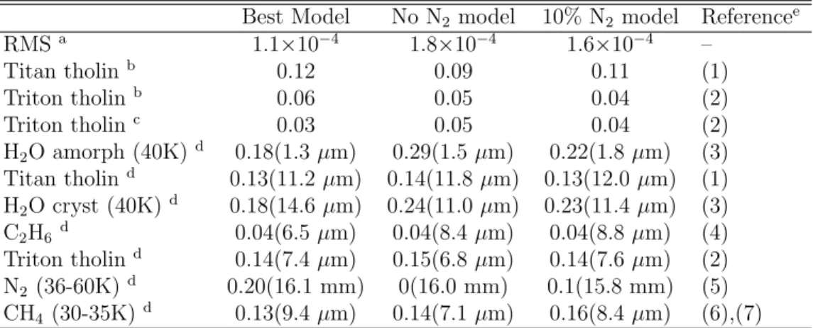
Table 4.3 – Best fitting model, model without N2, and model with 10% N2
for (50000) Quaoar. From Dalle Ore et al. (2009).
Best Model No N2 model 10% N2 model Referencee
RMSa 1.1×10⁻⁴ 1.8×10⁻⁴ 1.6×10⁻⁴ – Titan tholinb 0.12 0.09 0.11 (1) Triton tholin b 0.06 0.05 0.04 (2) Triton tholin c 0.03 0.05 0.04 (2) H2O amorph (40K)d 0.18(1.3 µm) 0.29(1.5 µm) 0.22(1.8 µm) (3) Titan tholind 0.13(11.2 µm) 0.14(11.8 µm) 0.13(12.0 µm) (1) H2O cryst (40K)d 0.18(14.6 µm) 0.24(11.0 µm) 0.23(11.4 µm) (3) C2H6d 0.04(6.5 µm) 0.04(8.4 µm) 0.04(8.8 µm) (4) Triton tholin d 0.14(7.4 µm) 0.15(6.8 µm) 0.14(7.6 µm) (2) N2(36-60K)d 0.20(16.1 mm) 0(16.0 mm) 0.1(15.8 mm) (5) CH4(30-35K)d 0.13(9.4 µm) 0.14(7.1 µm) 0.16(8.4 µm) (6),(7)
NOTE: All models were computed with a porosity of 0.1.
a
RMS error of each model when compared to the data.
b
Material mixed as inclusions in CH4 ice.
c
Material mixed as inclusions in crystalline H2O ice.
d
Material mixed intimately, with grain size in parenthesis. Temperature listed after the name of the component.
e
References: (1) Imanaka et al. (2005); (2) Khare et al. (1994); (3) Mastrapa & Sandford (2008); (4) Mastrapa (private comm.); (5) Green et al. (1991); (6) Grundy et al. (2002); (7) Hudgins et al. (1993).
since many of the parameters (optical costants, temperature and dilution of molecules in a matrix, etc.) are not well established or completely unknown. Moreover, mixtures with different grain sizes or different mixing ratios of the constituents can give very similar fits to the data. Nevertheless, the used models are generally able to describe the spectral properties of the analyzed objects quite well, and to put strong constraints on their surface composition. The best model
The best fitting (details in Table 4.3) for the spectrum of Quaoar consists of
an intimate mixture of crystalline and amorphous H2O, CH4, N2, and C2H6
ice, and of Triton and Titan tholins. Both crystalline H2O and CH4 ice are
contaminated molecularly by Triton and Titan tholins as well.
Starting with a mix of crystalline H2O and CH4 ices with reddening
ma-terials (tholins), a satisfactory fit was obtained up to 2.5µm, but caused the model to be too dark at the wavelengths of the Spitzer/IRAC bands by about 40%. Several attempts have been made to raise the albedo in this region, using a variety of materials, but they resulted in poor fits at shorter
0.0 0.2 0.4 0.6 0.8 1.0 0 1 2 3 4 5 6 Geometric Albedo Wavelength (µm) 0.4 0.5 0.6 0.7 0.8 1.0 1.2 1.4 1.6 1.8 2.0 2.2 2.4
Figure 4.5 – Best fitting model (solid line) for Quaoar, compared to a model
computed with the same components except amorphous H2O (dot-dashed
line). Open diamonds show the model convolved to the Spitzer filter response functions. Open triangles mark the first Spitzer exposure, open squares in-dicate the second. From Dalle Ore et al. (2009).
(brighter than crystalline H2O ice at the IRAC wavelengths) in extremely
small grains (∼ 1 µm), improving the fit by about 20% at 4.5µm. Fig. 4.5 shows both the best model (solid line) and the same fit calculated with no
amorphous H2O ice (dot-dashed line).
Molecular nitrogen has been included in the model, despite of the fact
that this component had never been detected on Quaoar before. N2 ice
improves the fit at 2.149 µm (Fig. 4.6), and also increases the albedo at 3.6
µm. Since the absorption bands of N2 ice are intrinsically weak, this material
could be present in relatively large amounts and escape direct spectroscopic detection.
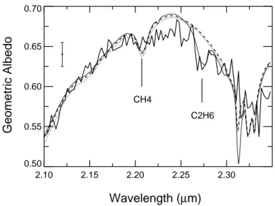
Moreover, based on previous works suggesting that NH4OH and C2H6
might be present on the surface of Quaoar (Jewitt & Luu 2004; Schaller & Brown 2007a), these have been introduced among the tentative components.
While the presence of NH4OH resulted to be unnecessary, a small amount
of C2H6 improves the fit to the small absorption at ≃ 2.27µm as shown in
Fig. 4.7.
These results permit to put strong constraints on the surface composition of (50000) Quaoar, one of the largest TNOs with its diameter of 1260 ± 190 km (Brown & Trujillo 2004). In particular, the unexpected abundance of the
4.1. SPECTROSCOPY AND MODELLING 69 2.00 2.05 2.10 2.15 2.20 2.25 0.45 0.50 0.55 0.60 0.65 0.70 Geometric Albedo Wavelength (µm) 20% N2 0% N2 N2 CH4
Figure 4.6 – Best fit (solid line) for Quaoar, and fit without N2 (dotted line).
The fit at 2.149 µm is moderately improved by the presence of 20% N2 ice.
From Dalle Ore et al. (2009).
highly volatile N2 makes this object peculiar, in this sense similar to Pluto
and Triton. Quaoar’s spectrum is however dominated by H2O ice, while CH4
is the major absorber in the spectra of Pluto and Triton. Schaller & Brown (2007b) have shown that Quaoar’s temperature and size put this object in a transition region between complete volatile loss and possible volatile reten-tion. Its reduced capability to retain very volatile species (compared to the
larger Pluto and Triton) could have led to a stronger presence of the H2O
ice, less volatile than CH4.
It has to be noted that also the best fitting model is too dark at the
Spitzer wavelengths, mainly because of the very absorbing crystalline H2O
ice. A possible solution could be found assuming a thin layer of amorphous
H2O ice covering the coarse mixture of the other components. This layer
could be due to the irradiation of the underneath crystalline water ice, but further laboratory experiments on ices and more developed spectral models are needed to test this hypothesis.
2.10 2.15 2.20 2.25 2.30 0.50 0.55 0.60 0.65 0.70 Geometric Albedo Wavelength (µm) C2H6 CH4
Figure 4.7 – Detail of the best fit for Quaoar (solid line), a fit without C2H6
(dashed), and a fit with NH4OH in place of C2H6 (dotted). There is some
evidence for C2H6 as shown by the fit to the 2.275µm band. NH4OH on the
other hand does not seem to contribute significantly (at this low concentra-tion). From Dalle Ore et al. (2009).
4.2
Colors and taxonomy
Because of the faintness of Trans-Neptunian Objects and Centaurs, spectro-scopic observations (which could provide the most detailed information about their surface compositions) are feasible only for a small number of them, even when using the largest ground-based telescopes (see Barucci et al. 2008a, for a recent review). Hence photometry is still the best tool to investigate the surface properties of a significant sample of these objects, allowing a global view of the whole known population.
Photometric surveys before the ESO-LP have observed about 200 ob-jects. Statistical analyses were performed to search for possible correlations between colors and physical and orbital parameters (for recent reviews, see Doressoundiram et al. 2008; Tegler et al. 2008). As the major result, a clus-tering of “cold” (low eccentricity, low inclination) classical TNOs with very red colors was found (see section 1.1).
4.2. COLORS AND TAXONOMY 71
4.2.1
Observations and data reduction
In the framework of the ESO-LP, visible and NIR photometry of TNOs and Centaurs has been performed at the ESO-VLT (Paranal, Chile). The data have been acquired during several observing runs, between October 2006 and November 2008. The observational circumstances are reported in Table 4.4. Visible photometry was performed with the two FORS instruments, using the broadband B, V , R, I filters, centered at 0.429, 0.554, 0.655 (or 0.657 in FORS2), and 0.768 µm, respectively.
NIR photometry was performed using the ISAAC instrument, with the J, H, Ks filters (central wavelength of 1.25, 1.65, and 2.16 µm, respectively). The images were reduced using the procedures described in sections 2.1.1 and 2.1.2.
4.2.2
Results
Visible and NIR photometric measurements have been obtained for 45 ob-jects, 19 of them have their colors reported for the first time ever.
Tables 4.5 and 4.6 list the resulting magnitude values, as well as the computed absolute magnitudes H of the targets, calculated as
H = V − 5 log (r∆) − αβ, (4.3)
where V represents the visible magnitude, ∆, r and α are the topocentric and heliocentric distances and the phase angle, respectively, and β is the phase curve slope (the term αβ is the correction for the opposition effect, e.g. Doressoundiram et al. 2008). For TNOs, it was assumed β = 0.14 ± 0.03 mag/deg, the modal value of the measurements published by Sheppard & Jewitt (2002). For Centaurs and Jupiter-coupled objects, it was assumed β = 0.11 ± 0.01 mag/deg, the result of a least squares fit by Doressoundiram
et al. (2005) of the linear phase function φ(α) = 10−αβ of data from Bauer
et al. (2003).
On the basis of the obtained color indices, the taxonomic classification of the targets was derived via the G-mode statistical method presented in Fulchignoni et al. (2000), using the taxonomy for TNOs and Centaurs in-troduced by Barucci et al. (2005a). As said in section 1.4.1, this taxonomy identifies four classes, that reasonably indicate different composition and/or evolutional history, with increasingly red colors: BB (neutral colors with respect to the Sun), BR, IR, RR (very red colors). The above-mentioned algorithm was applied to objects for which two or more color indices were available (i.e., to 41 out of the 45 observed TNOs and Centaurs).
Table 4.4 – Observational circumstances for Centaurs and TNOs whose colors have been obtained in the framework of the ESO-LP.
Object Date ∆ (AU) r(AU) α(deg)
(5145) Pholus 12 Apr 2008 21.212 21.864 2.0 (10199) Chariklo 20 Mar 2007 12.496 13.276 2.8 3 Feb 2008 13.311 13.395 4.2 4 Feb 2008 13.296 13.395 4.2 (20000) Varuna 4 Dec 2007 42.605 43.391 0.8 (26375) 1999 DE9 22 Jan 2007 34.767 35.435 1.2 (28978) Ixion 15 Jul 2007 41.241 42.019 0.9 (32532) Thereus 19 Sep 2007 10.345 11.006 4.1 (42301) 2001 UR163 5 Dec 2007 49.625 50.308 0.8 (42355) Typhon 24 Jan 2007 16.713 17.542 1.8 12 Apr 2008 16.892 17.650 2.2 (44594) 1999 OX3 21 Sep 2008 22.025 22.889 1.3 22 Sep 2008 22.033 22.888 1.3 (47171) 1999 TC36 9 Nov 2006 29.988 30.820 1.0 (47932) 2000 GN171 23 Jan 2007 28.378 28.352 2.0 24 Mar 2007 27.492 28.345 1.1 (50000) Quaoar 15 Jul 2007 42.449 43.267 0.8 (52872) Okyrhoe 3 Feb 2008 4.883 5.800 3.9 4 Feb 2008 4.877 5.800 3.7 (54598) Bienor 18 Sep 2007 17.127 18.116 0.6 (55565) 2002 AW197 23 Jan 2007 45.860 46.796 0.4 (55576) Amycus 12 Apr 2008 15.205 16.056 1.9 (55637) 2002 UX25 18 Sep 2007 41.188 42.004 0.8 6 Dec 2007 41.263 41.975 0.9 (55638) 2002 VE95 5 Dec 2007 27.297 28.248 0.5 6 Dec 2007 27.301 28.249 0.6 22 Nov 2008 27.379 28.341 0.5 23 Nov 2008 27.378 28.341 0.4 (60558) Echeclus 14 May 2007 11.239 12.124 2.4 (73480) 2002 PN34 10 Nov 2007 14.894 15.344 3.3 (83982) Crantor 14 Jul 2007 14.007 14.739 2.8 (90377) Sedna 21 Sep 2008 87.416 88.015 0.5 22 Sep 2008 87.402 88.014 0.5 (90482) Orcus 3 Feb 2008 46.904 47.807 0.5 4 Feb 2008 46.900 47.807 0.5 (90568) 2004 GV9 13 May 2007 38.141 39.069 0.6 (119951) 2002 KX14 13 Jul 2007 38.855 39.535 1.1 (120061) 2003 CO1 4 Feb 2008 10.937 11.080 5.1 12 Apr 2008 10.179 11.123 1.8 13 Apr 2008 10.175 11.123 1.8 (120132) 2003 FY128 22 Jan 2007 37.935 38.298 1.4 12 Apr 2008 37.477 38.454 0.3 (120178) 2003 OP32 21 Sep 2008 40.546 41.365 0.8 (120348) 2004 TY364 22 Nov 2008 38.840 39.591 0.9 23 Nov 2008 38.849 39.591 1.0 (136199) Eris 20 Oct 2006 95.837 96.798 0.2 19 Sep 2007 95.923 96.803 0.3 7 Dec 2007 96.226 96.792 0.5 (144897) 2004 UX10 4 Dec 2007 38.145 38.837 1.0 5 Dec 2007 38.158 38.837 1.1 6 Dec 2007 38.170 38.837 1.1 23 Nov 2008 38.059 38.879 0.8 (145451) 2005 RM43 19 Sep 2007 34.670 35.183 1.4 4 Dec 2007 34.298 35.195 0.7 7 Dec 2007 34.316 35.196 0.7 (145452) 2005 RN43 19 Sep 2007 39.837 40.714 0.7 (145453) 2005 RR43 18 Sep 2007 37.982 38.492 1.3 4 Dec 2007 37.623 38.511 0.6 7 Dec 2007 37.642 38.512 0.7 (174567) 2003 MW12 12 Apr 2008 47.314 47.968 0.9 13 Apr 2008 47.302 47.968 0.9 (208996) 2003 AZ84 24 Jan 2007 44.653 45.604 0.3 22 Nov 2008 44.879 45.458 1.0 23 Nov 2008 44.865 45.457 1.0 2002 KY14 21 Sep 2008 7.802 8.649 3.8 22 Sep 2008 7.810 8.649 3.8 2003 QW90 9 Nov 2006 43.426 44.156 0.9 2003 UZ117 25 Dec 2006 38.756 39.439 1.0 22 Nov 2008 38.420 39.368 0.4 23 Nov 2008 38.423 39.367 0.4 2003 UZ413 4 Dec 2007 41.171 42.004 0.7 21 Sep 2008 41.466 42.163 1.0 22 Nov 2008 41.276 42.197 0.5 23 Nov 2008 41.282 42.198 0.5 2007 UK126 21 Sep 2008 45.131 45.618 1.1 22 Sep 2008 45.117 45.617 1.1 2007 UM126 21 Sep 2008 10.202 11.163 1.5 22 Sep 2008 10.199 11.165 1.5 2007 VH305 22 Nov 2008 7.854 8.638 4.2 23 Nov 2008 7.863 8.636 4.3 2008 FC76 20 Sep 2008 10.968 11.690 3.5 21 Sep 2008 10.976 11.688 3.6 2008 SJ236 22 Nov 2008 5.522 6.364 5.0 23 Nov 2008 5.530 6.363 5.1
NOTE: ∆, r and α are the topocentric distance, the heliocentric distance, and the phase angle, respectively.
4.2. COLORS AND TAXONOMY 73
Table 4.5 – Observed magnitudes, first year of the ESOLP (October 2006 -September 2007). From DeMeo et al. (2009b).
Object Date UTST ART B V R I J H Ks HV
(10199) Chariklo 20 Mar 2007 03:22 ... 18.49±0.05 18.04±0.07 ... 17.00±0.05 16.51±0.06 16.30±0.06 7.09±0.05 (26375) 1999 DE9 22 Jan 2007 05:48 ... 20.75±0.04 20.13±0.02 19.63±0.02 19.22±0.06 18.93±0.07 18.87±0.07 5.13±0.05 (28978) Ixion 15 Jul 2007 02:47 ... 20.22±0.05 19.67±0.06 ... 18.63±0.04 18.37±0.05 18.38±0.05 3.90±0.06 (32532) Thereus 19 Sep 2007 06:44 20.71±0.05 19.90±0.03 ... 19.00±0.13 18.55±0.04 18.15±0.06 18.04±0.06 9.18±0.03 (42355) Typhon 24 Jan 2007 05:33 ... 20.34±0.02 19.87±0.02 19.41±0.02 18.78±0.04 18.33±0.05 18.17±0.05 7.75±0.04 24 Jan 2007 05:46 ... 20.36±0.02 19.88±0.02 19.41±0.02 ... ... ... 7.77±0.04 (47171) 1999 TC36 9 Nov 2006 00:58 ... 20.25±0.03 ... 19.00±0.03 18.17±0.07 17.85±0.07 17.79±0.08 5.25±0.04 9 Nov 2006 01:09 ... 20.26±0.03 ... 19.00±0.03 ... ... ... 5.26±0.04 (47932) 2000 GN171 23 Jan 2007 07:06 ... 21.01±0.03 20.42±0.02 19.91±0.02 19.43±0.08 19.09±0.09 ... 6.20±0.04 23 Jan 2007 07:15 ... 21.04±0.03 20.42±0.02 19.90±0.02 ... ... ... 6.23±0.04 24 Jan 2007 07:17 ... 21.11±0.03 20.54±0.02 19.99±0.02 19.42±0.06 19.04±0.07 18.98±0.07 6.30±0.04 24 Jan 2007 07:26 ... 21.12±0.03 20.54±0.02 20.00±0.02 ... ... ... 6.31±0.04 24 Mar 2007 05:12 ... 21.30±0.06 20.73±0.08 ... ... ... ... 6.69±0.07 ∗(50000) Quaoar 15 Jul 2007 01:33 ... 19.25±0.05 18.65±0.05 ... 17.07±0.03 16.71±0.04 16.68±0.04 2.82±0.06 (54598) Bienor 18 Sep 2007 04:05 20.71±0.05 19.98±0.03 ... 19.05±0.16 18.46±0.05 18.09±0.05 ... 7.46±0.03 (55565) 2002 AW197 23 Jan 2007 05:13 ... 20.36±0.02 19.76±0.02 19.21±0.02 18.62±0.05 18.28±0.06 18.21±0.06 3.65±0.04 23 Jan 2007 05:25 ... 20.37±0.02 19.76±0.02 19.21±0.02 ... ... ... 3.66±0.04 (55637) 2002 UX25 18 Sep 2007 06:50 21.31±0.23 20.28±0.06 ... 19.12±0.34 ... ... ... 3.98±0.07 (60558) Echeclus 14 May 2007 00:51 ... 20.61±0.06 20.12±0.07 ... 19.13±0.04 18.76±0.06 18.42±0.09 9.67±0.06 (83982) Crantor 14 Jul 2007 01:32 ... 21.00±0.07 20.27±0.08 ... ... ... ... 9.12±0.07 16 Jul 2007 01:03 ... 20.91±0.02 20.17±0.03 ... ... ... ... 9.01±0.02 ∗(90568) 2004 GV 9 13 May 2007 02:14 ... 20.20±0.03 19.64±0.03 ... 18.63±0.05 18.29±0.08 18.15±0.05 4.25±0.04 ∗(119951) 2002 KX 14 13 Jul 2007 01:29 ... 20.95±0.08 20.34±0.04 ... ... ... ... 4.86±0.09 ∗(120132) 2003 FY 128 22 Jan 2007 06:49 ... 21.06±0.03 20.47±0.02 19.91±0.02 19.42±0.05 19.06±0.06 18.95±0.06 5.05±0.04 22 Jan 2007 07:01 ... 21.06±0.03 20.47±0.02 19.91±0.02 ... ... ... 5.05±0.04 (136199) Eris 19 Sep 2007 05:24 19.59±0.06 18.74±0.04 ... 18.01±0.12 17.96±0.04 17.88±0.06 18.16±0.06 -1.14±0.05 20 Oct 2006 04:24 ... 18.74±0.02 ... 18.00±0.02 17.79±0.08 ... ... -1.13±0.04 20 Oct 2006 05:49 ... 18.75±0.02 ... 17.99±0.02 ... ... ... -1.12±0.04 ∗(145451) 2005 RM 43 19 Sep 2007 09:17 20.88±0.06 20.18±0.03 ... 19.48±0.18 19.27±0.06 19.07±0.06 18.79±0.07 4.55±0.04 ∗(145452) 2005 RN 43 19 Sep 2007 03:23 21.05±0.07 20.02±0.03 ... 18.89±0.21 18.47±0.05 18.16±0.05 17.97±0.05 3.87±0.04 19 Sep 2007 04:04 ... ... ... ... 18.39±0.05 ... ... ... ∗(145453) 2005 RR 43 18 Sep 2007 06:50 20.79±0.12 20.08±0.03 ... 19.32±0.16 19.06±0.06 ... ... 4.07±0.04 18 Sep 2007 07:33 ... ... ... ... 19.12±0.06 ... ... ... (208996) 2003 AZ84 24 Jan 2007 03:38 ... 20.33±0.02 19.93±0.02 19.60±0.02 19.12±0.05 18.81±0.05 18.75±0.05 3.74±0.04 24 Jan 2007 03:47 ... 20.33±0.02 19.94±0.02 19.60±0.02 ... ... ... 3.74±0.04 ∗2003 QW 90 9 Nov 2006 02:19 ... 21.80±0.06 ... 20.69±0.05 19.87±0.15 ... ... 5.25±0.07 9 Nov 2006 02:45 ... 21.82±0.06 ... 20.69±0.05 ... ... ... 5.27±0.07 ∗2003 UZ 117 25 Dec 2006 01:02 ... 21.25±0.04 ... 20.58±0.03 ... ... ... 5.16±0.05 25 Dec 2006 02:18 ... 21.26±0.04 ... 20.59±0.04 ... ... ... 5.17±0.05
Table 4.6 – Observed magnitudes, second year of the ESO-LP (November 2007 - November 2008). From Perna et al. (2010a), and references therein.
Object Date UTST ART V R I J H Ks HV
(5145) Pholus 12 Apr 2008 05:48 21.33 ± 0.09 20.64 ± 0.09 19.95 ± 0.15 ... ... ... 7.78 ± 0.09 (10199) Chariklo 3 Feb 2008 07:41 ... ... ... 17.11 ± 0.06 16.61 ± 0.05 16.38 ± 0.06 ... 4 Feb 2008 07:41 18.79 ± 0.02 18.34 ± 0.02 17.88 ± 0.03 ... ... ... 7.07 ± 0.04 (20000) Varuna 4 Dec 2007 06:09 20.49 ± 0.03 19.88 ± 0.03 ... ... ... ... 4.04 ± 0.04 4 Dec 2007 06:12 20.46 ± 0.04 19.88 ± 0.03 ... ... ... ... 4.01 ± 0.05 (42301) 2001 UR163 5 Dec 2007 00:52 21.82 ± 0.06 20.98 ± 0.07 ... ... ... ... 4.72 ± 0.06 5 Dec 2007 00:55 21.81 ± 0.05 20.98 ± 0.07 ... ... ... ... 4.71 ± 0.06 (42355) Typhon 12 Apr 2008 00:59 20.50 ± 0.08 20.00 ± 0.08 19.70 ± 0.08 ... ... ... 7.77 ± 0.11 (44594) 1999 OX3 21 Sep 2008 04:07 21.26 ± 0.05 20.54 ± 0.06 19.96 ± 0.07 ... ... ... 7.57 ± 0.06 22 Sep 2008 04:49 ... ... ... 19.08 ± 0.12 18.75 ± 0.08 18.69 ± 0.08 ... (52872) Okyrhoe 3 Feb 2008 06:41 ... ... ... 16.84 ± 0.06 16.39 ± 0.07 16.28 ± 0.05 ... 4 Feb 2008 06:18 18.63 ± 0.02 18.14 ± 0.02 17.64 ± 0.02 ... ... ... 10.97 ± 0.04 (55576) Amycus 12 Apr 2008 03:33 20.42 ± 0.08 19.78 ± 0.08 19.20 ± 0.15 ... ... ... 8.27 ± 0.08 (55637) 2002 UX25 6 Dec 2007 01:19 ... ... ... 18.55 ± 0.03 18.25 ± 0.04 18.21 ± 0.06 ... (55638) 2002 VE95 5 Dec 2007 03:35 20.31 ± 0.03 19.59 ± 0.04 ... ... ... ... 5.80 ± 0.03 5 Dec 2007 03:38 20.31 ± 0.03 19.59 ± 0.04 ... ... ... ... 5.80 ± 0.03 6 Dec 2007 02:09 ... ... ... 18.11 ± 0.04 17.78 ± 0.04 17.74 ± 0.04 ... 22 Nov 2008 05:36 20.28 ± 0.06 19.53 ± 0.08 18.77 ± 0.09 ... ... ... 5.76 ± 0.06 23 Nov 2008 05:57 ... ... ... 18.04 ± 0.07 17.68 ± 0.07 17.63 ± 0.09 ... (73480) 2002 PN34 10 Nov 2007 00:36 20.68 ± 0.03 20.25 ± 0.05 ... 19.00 ± 0.05 18.49 ± 0.06 18.29 ± 0.05 8.42 ± 0.10 (90377) Sedna 21 Sep 2008 06:33 21.34 ± 0.04 20.57 ± 0.05 19.93 ± 0.05 ... ... ... 1.84 ± 0.04 22 Sep 2008 06:57 ... ... ... 19.20 ± 0.04 18.78 ± 0.06 ... ... (90482) Orcus 3 Feb 2008 04:46 ... ... ... 17.91 ± 0.05 17.72 ± 0.07 17.89 ± 0.05 ... 4 Feb 2008 05:04 19.12 ± 0.02 18.73 ± 0.02 18.37 ± 0.02 ... ... ... 2.30 ± 0.03 (120061) 2003 CO1 4 Feb 2008 08:17 19.93 ± 0.02 19.45 ± 0.03 19.01 ± 0.03 ... ... ... 8.95 ± 0.05 12 Apr 2008 04:40 19.63 ± 0.08 19.20 ± 0.09 18.82 ± 0.15 ... ... ... 9.16 ± 0.08 (120132) 2003 FY128 12 Apr 2008 02:22 20.93 ± 0.09 20.34 ± 0.09 19.86 ± 0.15 ... ... ... 5.09 ± 0.09 ∗(120178) 2003 OP 32 21 Sep 2008 02:10 20.25 ± 0.03 19.86 ± 0.05 19.50 ± 0.05 ... ... ... 4.02 ± 0.04 (120348) 2004 TY364 22 Nov 2008 04:32 20.64 ± 0.03 20.04 ± 0.04 19.52 ± 0.04 ... ... ... 4.58 ± 0.04 23 Nov 2008 03:22 ... ... ... 18.87 ± 0.03 18.42 ± 0.05 18.39 ± 0.08 ... (136199) Eris 7 Dec 2007 00:20 ... ... ... 17.90 ± 0.06 17.85 ± 0.05 18.15 ± 0.06 ... ∗(144897) 2004 UX 10 4 Dec 2007 00:53 20.61 ± 0.04 20.04 ± 0.04 ... ... ... ... 4.62 ± 0.05 4 Dec 2007 00:56 20.63 ± 0.04 20.05 ± 0.04 ... ... ... ... 4.64 ± 0.05 5 Dec 2007 02:24 20.63 ± 0.03 20.06 ± 0.04 ... ... ... ... 4.62 ± 0.04 6 Dec 2007 00:39 ... ... ... 18.97 ± 0.06 18.55 ± 0.08 18.55 ± 0.09 ... 23 Nov 2008 02:26 ... ... ... 19.02 ± 0.03 18.60 ± 0.04 18.64 ± 0.06 ... (145451) 2005 RM43 4 Dec 2007 03:22 20.04 ± 0.04 19.66 ± 0.03 ... ... ... ... 4.53 ± 0.05 4 Dec 2007 03:25 20.07 ± 0.04 19.66 ± 0.03 ... ... ... ... 4.56 ± 0.05 7 Dec 2007 03:14 ... ... ... 18.95 ± 0.04 18.76 ± 0.05 18.71 ± 0.06 ... (145453) 2005 RR43 4 Dec 2007 02:26 20.05 ± 0.03 19.66 ± 0.04 ... ... ... ... 4.16 ± 0.03 4 Dec 2007 02:29 20.08 ± 0.03 19.66 ± 0.04 ... ... ... ... 4.19 ± 0.03 7 Dec 2007 02:24 ... ... ... 19.28 ± 0.04 19.47 ± 0.07 19.67 ± 0.15 ... ∗(174567) 2003 MW 12 12 Apr 2008 07:07 20.57 ± 0.08 19.99 ± 0.08 19.57 ± 0.15 ... ... ... 3.66 ± 0.08 (208996) 2003 AZ84 22 Nov 2008 06:07 20.46 ± 0.03 20.08 ± 0.04 19.71 ± 0.03 ... ... ... 3.77 ± 0.04 23 Nov 2008 07:10 ... ... ... 19.26 ± 0.04 18.92 ± 0.07 ... ... ∗2002 KY 14 21 Sep 2008 00:56 19.93 ± 0.02 19.23 ± 0.03 18.58 ± 0.04 ... ... ... 10.37 ± 0.04 22 Sep 2008 02:27 ... ... ... 17.85 ± 0.06 17.56 ± 0.07 17.54 ± 0.08 ... 2003 UZ117 22 Nov 2008 03:21 21.13 ± 0.03 20.77 ± 0.04 20.43 ± 0.04 ... ... ... 5.18 ± 0.03 23 Nov 2008 05:08 ... ... ... 20.41 ± 0.09 20.63 ± 0.17 ... ... ∗2003 UZ 413 4 Dec 2007 04:28 20.70 ± 0.04 20.22 ± 0.04 ... ... ... ... 4.41 ± 0.05 4 Dec 2007 04:31 20.67 ± 0.04 20.22 ± 0.04 ... ... ... ... 4.38 ± 0.05 21 Sep 2008 05:31 20.71 ± 0.04 20.25 ± 0.05 19.88 ± 0.06 ... ... ... 4.36 ± 0.05 22 Nov 2008 03:33 20.63 ± 0.03 20.22 ± 0.04 19.82 ± 0.04 ... ... ... 4.36 ± 0.03 23 Nov 2008 04:03 ... ... ... 19.29 ± 0.05 18.92 ± 0.09 18.77 ± 0.09 ... ∗2007 UK 126 21 Sep 2008 08:05 20.41 ± 0.03 19.79 ± 0.04 19.32 ± 0.04 ... ... ... 3.69 ± 0.04 22 Sep 2008 07:43 ... ... ... 18.88 ± 0.07 18.52 ± 0.08 ... ... ∗2007 UM 126 21 Sep 2008 04:26 20.88 ± 0.03 20.44 ± 0.03 20.00 ± 0.03 ... ... ... 10.43 ± 0.03 22 Sep 2008 05:57 ... ... ... ... 18.84 ± 0.13 18.50 ± 0.08 ... ∗2007 VH 305 22 Nov 2008 02:14 21.44 ± 0.04 20.96 ± 0.04 20.48 ± 0.05 ... ... ... 11.82 ± 0.06 23 Nov 2008 00:38 ... ... ... 19.70 ± 0.10 19.06 ± 0.12 19.43 ± 0.15 ... ∗2008 FC 76 20 Sep 2008 23:55 20.38 ± 0.03 19.67 ± 0.05 19.04 ± 0.06 ... ... ... 9.46 ± 0.05 21 Sep 2008 23:53 ... ... ... 18.40 ± 0.08 18.00 ± 0.08 17.88 ± 0.09 ... ∗2008 SJ 236 22 Nov 2008 00:24 20.75 ± 0.03 20.13 ± 0.03 19.63 ± 0.04 ... ... ... 12.47 ± 0.06 23 Nov 2008 01:28 ... ... ... 19.01 ± 0.07 18.60 ± 0.11 18.83 ± 0.12 ...
4.2. COLORS AND TAXONOMY 75 Each object has been classified whenever its colors were within 3σ of the class’ average values. Obviously, a higher number of available colors implies a better reliability of the class determination. In cases where more than one class is within 3σ, a multiple designation was assigned to the object, with taxonomic classes ordered by ascending deviation of its colors from the class’ averages. The obtained taxonomic designations are reported in Table 4.7, along with the dynamical classification of the objects (according to Gladman et al. 2008). Thirty-eight objects have been classified: nine of them turned out to belong to the BB class, seven were BR, ten were RR. The remaining twelve targets got a multiple designation.
Three objects, 2007 UK126, (26375) 1999 DE9, and (145452) 2005 RN43,
did not fall within any class of the existing taxonomy. Indeed, according to their visible colors an IR, RR classification could be derived, while their infrared colors match those of a BB, BR object. This fact, as well as the presence of several multiple classifications, could support the idea that further groups could be found as the number of analysed objects increases, leading to a refinement of the current taxonomy.
Below, objects that showed a peculiar behavior are discussed in further detail.
(10199) Chariklo: Using five color indices, this Centaur has been classified
as a BR object, as Fulchignoni et al. (2008) did on the basis of the mean colors published in literature. The results in Perna et al. (2010a), obtained in February 2008 (and already published in Guilbert et al. 2009), agree with these average measurements except for the V − K color which is about 0.2 magnitudes redder in the 2008 dataset. Interestingly, Chariklo was already observed in the framework of the ESO-LP programme in March 2007 (DeMeo et al. 2009b, who assigned to Chariklo a BR, BB classification), but no match is found with these previous results (compare values in Tables 4.5 and 4.6). Since the acquisition and the reduction of the data were carried out in the same way in both observing runs, this is a probable indication of heterogeneity on the surface of this Centaur, as already proposed in previous works (see Guilbert et al. 2009, and references therein).
(90377) Sedna: The photometric colors and taxonomic classification (RR)
derived for Sedna are in agreement with those published by Barucci et al. (2005b), except for the V − J color which is approximately 0.2 magnitudes bluer in the ESO-LP dataset. Since images in different filters have not been acquired simultaneously, the observation of different rotational phases of the object could affect color determinations. Nevertheless the light curve
Table 4.7 – Taxonomic classification of Centaurs and TNOs obtained within the ESO Large Programme.
Object Dyn. Class Taxonomy N
Fulchignoni et al. (2008) DeMeo et al. (2009b) Perna et al. (2010a)
(5145) Pholus Centaur RR ... RR 2
(10199) Chariklo Centaur BR BR,BB BR 5 (42355) Typhon Scattered BR BR BR,BB 5a (44594) 1999 OX3 Scattered RR ... RR 5 (52872) Okyrhoe Jupiter-coupled BR ... BR,IR 5 (55576) Amycus Centaur RR ... RR,IR 2 (55637) 2002 UX25 Classical IR RR,IR RR 5b (55638) 2002 VE95 Resonant (3:2) RR ... RR 5 (73480) 2002 PN34 Scattered ... ... BR,BB 4 (90377) Sedna Detached RR ... RR 4 (90482) Orcus Resonant (3:2) BB ... BB 5 (120061) 2003 CO1 Centaur ... ... BR 2 (120132) 2003 FY128 Detached ... BR BR 5a (120178) 2003 OP32 Classical ... ... BB,BR 2 (120348) 2004 TY364 Classical ... ... IR,RR,BR 5 (136199) Eris Detached BB BB BB 5b (144897) 2004 UX10 Classical ... ... BR 4 (145451) 2005 RM43 Detached ... BB BB 4 (145453) 2005 RR43 Classical ... BB BB 4 (174567) 2003 MW12 Classical ... ... IR,BR,RR 2 (208996) 2003 AZ84 Resonant (3:2) BB BB BB 4 2002 KY14 Centaur ... ... RR 5 2003 UZ117 Classical ... ... BB 4 2003 UZ413 Resonant (3:2) ... ... BB 5 2007 UM126 Centaur ... ... BR,BB 4 2007 VH305 Centaur ... ... BR 5 2008 FC76 Centaur ... ... RR 5 2008 SJ236 Centaur ... ... RR 5 (28978) Ixion Resonant (3:2) IR BB 4 (32532) Thereus Centaur BR BB 5 (47171) 1999 TC36 Resonant (3:2) RR RR 4 (47932) 2000 GN171 Resonant (3:2) IR BR,IR 5 (50000) Quaoar Classical ... RR 4 (54598) Bienor Centaur BR BR 4
(55565) 2002 AW197 Classical IR IR,RR 5 (60558) Echeclus Jupiter-coupled BR BR,BB 4 (90568) 2004 GV9 Classical ... BR 4
2003 QW90 Classical ... IR,RR,BR 2
NOTE: In the statistical analysis of taxa, for the first 28 bodies the classification from Perna et al. (2010a) is taken into account. Last 10 objects come from DeMeo et al. (2009b). N is the number of colors used to classify each object, by Perna et al. (2010a) or DeMeo et al. (2009b).
a Using near-infrared data from DeMeo et al. (2009b).
b Using visible data from DeMeo et al. (2009b).
of Sedna has an amplitude of only 0.02 magnitudes (Gaudi et al. 2005), hence different observed silhouettes of the body cannot explain the found discrepancy, which could instead be attributed to surface heterogeneity.
4.2. COLORS AND TAXONOMY 77
(145451) 2005 RM43: Both datasets obtained in the framework of the
ESO-LP give a BB classification, even if both V − J and V − H colors are ∼ 0.2 magnitudes redder in Perna et al. (2010a) than in DeMeo et al. (2009b), while the V − K color is consistent. Observations with different filters have not been carried out simultaneously, but, as for Sedna, the amplitude of the light curve is smaller than the observed discrepancies (∆m = 0.12 ± 0.05 magnitudes; Perna et al. 2009, see section 4.3), suggesting possible surface heterogeneity.
(145453) 2005 RR43: Observed twice during the ESO-LP, Perna et al. (2010a)
confirm that 2005 RR43is a BB object, as classified by DeMeo et al. (2009b),
but in the former work the V − H color is 0.4 magnitudes bluer than pub-lished by the latter. Again, images with different filters have not been ac-quired at the same moment but the amplitude of the light curve is only ∆m = 0.12 ± 0.03 magnitudes (Perna et al. 2009, see section 4.3), so the observation of different compositions on the surface is a likely explanation for the reported discrepancy.
(26375) 1999 DE9: Seven measurements combined in Fulchignoni et al.
(2008) produced the previous classification (IR) of 1999 DE9. Considering
that light curve data do not indicate significant magnitude variations (Shep-pard & Jewitt 2002), it appears that previous measurements were robust and
stable. As said above, 1999 DE9 did not fall within any taxon on the basis of
the ESO-LP data (five color indices). While the obtained visible colors agree with published results, the V − J, V − H, V − K colors are approximately 0.3 magnitudes bluer. The J − H and J − K colors, however, are in good agreement with previous works (Doressoundiram et al. 2007; Delsanti et al.
2006). Jewitt & Luu (2001) noted a spectral feature attributed to H2O ice
(abundance around 10%), which was also detected by Barkume et al. (2008). This feature was not seen by Doressoundiram et al. (2003), suggesting that there may be heterogeneity on the surface.
(29878) Ixion: Ixion had been classified by Fulchignoni et al. (2008) as an
IR object, based on a set of six colors from Doressoundiram et al. (2007), while it is a BB-type according to the ESO-LP data (four colors). Obtained V − J and V − H colors were each almost 0.3 magnitudes lower than seen by Doressoundiram et al. (2007), which produced the significant classification change (J − H color agrees with the above cited work, while the J − K is slightly redder). This body does not have a significant light curve amplitude (Sheppard & Jewitt 2003; Ortiz et al. 2003), so the observed discrepancies may correspond to surface heterogeneity.
(32532) Thereus: The Centaur Thereus was previously classified as a BR
object (Fulchignoni et al. 2008), while the ESO-LP data classify it as a BB-type. Though the obtained visible magnitudes agree with published results, the V − J, V − H, and V − K colors are, respectively, more than 0.3, almost 0.4, and ∼ 0.45 magnitudes bluer than the average values published by Fulchignoni et al. (2008). These differences are striking. Thereus has a double peaked light curve of amplitude 0.18 magnitudes. Moreover, the rotational period is of 8.34 hours (Farnham & Davies 2003), while ESO-LP visible and NIR measurements were taken only 11 minutes apart, so the difference cannot be attributed to observing different parts of the surface. Merlin et al. (2005) report significant spectral variation across the surface, which could rather account for the reported discrepancy.
(47932) 2000 GN171: This object has been classified as a BR, IR, which is
consistent with the previous result (IR) by Fulchignoni et al. (2008). Though
a homogeneous surface composition has been suggested for 2000 GN171
(Mer-lin et al. 2005), the calculated absolute magnitude Hv ranges from 6.20 to
6.31 ± 0.04 depending on the night of observation, while Doressoundiram
et al. (2007) reports Hv = 6.71 ± 0.05 and McBride et al. (2003) found a
sim-ilar value of 6.71 ± 0.04. Moreover, the V − J, V − H, and V − K colors are, respectively, ∼ 0.2, ∼ 0.2, and ∼ 0.3 magnitudes bluer than the averages computed by Fulchignoni et al. (2008). Nevertheless the observed discep-ancies are well within the amplitude of the light curve (∼ 0.6 magnitudes, Sheppard & Jewitt 2002; Perna et al. 2009, see section 4.3).
(54598) Bienor: The calculated absolute magnitude Hv is 7.46 ± 0.03, while
Doressoundiram et al. (2007) obtained Hv = 8.04 ± 0.02. This large
differ-ence is still smaller than the light curve amplitude of 0.75 ± 0.09 magnitudes (while the period is 4.57 ± 0.02 hours, Ortiz et al. 2002). Visible and NIR observations were taken approximately 45 minutes apart, a time span dur-ing which the object rotated significantly, which could also account for the observed difference.
4.2.3
Statistical analysis
Before the ESO-LP, Fulchignoni et al. (2008) classified all of the 132 TNOs and Centaurs for which data from the literature were available (one more
object, 1998 WU24, was classified as BR; but it has an unusual orbit, it is
not a Centaur, and therefore I do not consider it in the analysis). Of the 38 objects for which the taxonomy has been derived in the framework of the
4.2. COLORS AND TAXONOMY 79 ESO-LP, 19 of them have been classified for the first time (which constitutes about a 14% increase of the sample), while 4 targets were assigned different classes with respect to the results by Fulchignoni et al. (2008).
Considering the total sample of 151 objects, the average colors of each taxon were obtained. They are reported in Table 4.8 and represented in Fig. 4.8 as reflectance values normalized to the Sun and to the V colors. In the cases where multiple taxonomic classes were assigned to an object, only the first designation was taken into account. Then, the distribution of the four taxonomic groups with respect to the dynamical properties of the objects was analysed.
Table 4.8 – Average colors of the four TNO taxa.
Class B − V V − R V − I V − J V − H V − K
BB 0.68 ± 0.06 0.39 ± 0.05 0.75 ± 0.06 1.20 ± 0.25 1.28 ± 0.50 1.32 ± 0.60
BR 0.75 ± 0.06 0.49 ± 0.05 0.96 ± 0.08 1.68 ± 0.15 2.11 ± 0.14 2.26 ± 0.13
IR 0.92 ± 0.05 0.59 ± 0.04 1.15 ± 0.07 1.86 ± 0.06 2.20 ± 0.09 2.29 ± 0.10
RR 1.06 ± 0.10 0.69 ± 0.06 1.35 ± 0.10 2.22 ± 0.20 2.58 ± 0.25 2.59 ± 0.28
NOTE: All of the 151 Centaurs and TNOs that have been classified thus far are taken into account. In the cases where multiple taxonomic classes were assigned to an object, the first designation is considered.
First of all, the sampling of the taxa within each dynamical class (Fig. 4.9) was verified. The well-known color bimodality of Centaurs clearly emerges, since 13 out of 25 objects belong to the BR group, while 10 of them fall in the RR class. All of the four new IR-classified objects are classical TNOs, confirming the finding that IR objects seem to be concentrated in the reso-nant and classical dynamical classes, as stated by Fulchignoni et al. (2008). As reported by the same authors, RR objects dominate the classical TNOs. However, the classical TNOs in the objects constituting the ESO-LP sample do not conform to this behavior, as a quite equal division of the four taxa appears among them (check Table 4.7).
In Fig. 4.10 the distribution of taxonomical classes with respect to the semimajor axes a of the objects is presented. A 10 AU binning is adopted (nine objects are out of the scale). As already noted by Fulchignoni et al. (2008), the more distant TNOs belong to all the four taxa in a quite uniform
way, while for a <∼ 30 AU the BR and RR classes dominate the population.
Finally, Fig. 4.11 reports the distribution of the taxa with respect to
the orbital inclination i. A 5◦ binning is adopted (two objects are out of
the scale). Inclinations of RR-types are quite low, in agreement with the previously mentioned finding of a red dynamically “cold” population. On the
Figure 4.8 – Average reflectance values for each TNO taxon, normalized to the Sun and to the V colors. From Perna et al. (2010a).
Figure 4.9 – Distribution of the TNO taxa within each dynamical class, as defined by Gladman et al. (2008). From Perna et al. (2010a).
4.2. COLORS AND TAXONOMY 81
Figure 4.10 – Distribution of the TNO taxa with respect to the semimajor axis of the objects. A 10 AU binning is adopted. From Perna et al. (2010a).
Figure 4.11 – Distribution of the TNO taxa with respect to the orbital
contrary, BB-types seem to be concentrated at high inclinations, confirming the suggested association of these objects with the “hot” population.
As suggested by Fulchignoni et al. (2008), it is possible to interpret the different TNO taxa both in terms of evolution of the population and/or in terms of original differences in the composition of the objects.
In the former case, the “trend” connecting the BB taxon to the RR taxon would indicate the time during which an object has been exposed to different alteration processes (induced by collisions and/or space weathering), and each taxon represents a different stage in the evolution of the population.
In terms of original compositional differences, the dichotomy between the “hot” BB-types and the “cold” RR-types would be real. In this case, BR and IR objects would represent the space weathered evolution of BB and RR objects, respectively. As explained in section 1.2.2.2, the energetic particle bombardment of “dirty” icy surfaces induces the formation of dark, spectrally red hydrocarbons, which could be considered to be responsible for the BB → BR transition. Conversely, the induced loss of carbonaceous volatiles would result in objects being less red than they were previously, hence in the RR → IR transition.
4.3
Light curves and densities
The most useful tool for investigating the rotational properties of TNOs and for computing the axis ratios of the osculating ellipsoids approximating their shapes is the analysis of photometric light curves, which also allows us to retrieve useful information on the internal structure of each observed body (see section 1.4.3).
4.3.1
Observations and data reduction
To increase the still rather limited sample of TNOs with known rotational properties (few tens of objects, for a review see Sheppard et al. 2008), in the framework of the ESO-LP two observing runs (3 nights each) have been carried out in April 2007 and December 2007 at the ESO-NTT (La Silla, Chile).
The observations have been performed using the EMMI (ESO Multi-Mode Instrument) instrument in RILD (“red”) mode. The R filter (centered on 641.0 nm) was used, adjusting the exposure time according to the object magnitude and sky conditions.
4.3. LIGHT CURVES AND DENSITIES 83
In April 2007 data have been obtained on 2 Centaurs, (12929) 1999 TZ1
and (95626) 2002 GZ32, and 5 Trans-Neptunian Objects: (42355) Typhon,
(47932) 2000 GN171, (65489) Ceto, (90568) 2004 GV9, and (120132) 2003
FY128. Five additional TNOs have been studied during the second run:
(144897) 2004 UX10, (145451) 2005 RM43, (145453) 2005 RR43, 2003 UZ117,
and 2003 UZ413.
Table 4.9 reports the dynamical classification (according to Gladman et al. 2008) and the absolute magnitude H (reported by the Minor Planet Center) of each observed target.
Table 4.9 – TNOs and Centaurs whose light curves have been obtained in the framework of the ESO-LP.
Object Dyn. class. H
(12929) 1999 TZ1 Trojan/Centaur 9.3
(42355) Typhon Scattered TNO 7.2
(47932) 2000 GN171 Resonant TNO 6.0
(65489) Ceto Scattered TNO 6.3
(90568) 2004 GV9 Classical TNO 4.0 (95626) 2002 GZ32 Centaur 6.8 (120132) 2003 FY128 Detached TNO 5.0 (144897) 2004 UX10 Classical TNO 4.7 (145451) 2005 RM43 Detached TNO 4.4 (145453) 2005 RR43 Classical TNO 4.0 2003 UZ117 Classical TNO 5.3 2003 UZ413 Resonant TNO 4.3
The images were reduced using standard procedures (see section 2.1.1), but because of the non-photometric sky conditions, an absolute calibration of the magnitudes, by means of observing standard stars, was impossible. Therefore, differential photometry with bright (to minimize random errors) field stars was performed, typically using three of them within each image.
By visual inspection and radial profile analysis of the images, a search for possible signatures of a faint coma around the observed TNOs have been performed, but none were found.
The obtained (light-time corrected) single-night light curves are presented in Figs. 4.12 and 4.13.
12929 1999 TZ1 (17 Apr 07) 0 2 4 6 8 10 Hours 0.5 0.4 0.3 0.2 0.1 0.0 Delta-R 42355 Typhon (18 Apr 07) 20 21 22 23 0 1 2 3 Hours 2.70 2.60 2.50 2.40 2.30 2.20 2.10 Delta-R 42355 Typhon (19 Apr 07) 20 21 22 23 0 1 2 3 Hours 4.00 3.90 3.80 3.70 3.60 3.50 Delta-R 47932 2000 GN171 (17 Apr 07) 20 22 0 2 4 6 Hours 3.4 3.2 3.0 2.8 2.6 2.4 2.2 Delta-R 47932 2000 GN171 (18 Apr 07) 20 22 0 2 4 6 Hours 4.4 4.2 4.0 3.8 3.6 3.4 3.2 Delta-R 120132 2003 FY128 (18 Apr 07) 18 20 22 0 2 4 Hours 4.30 4.20 4.10 4.00 3.90 3.80 3.70 Delta-R 90568 2004 GV9 (18 Apr 07) 18 20 22 0 2 4 Hours 3.2 3.1 3.0 Delta-R 90568 2004 GV9 (19 Apr 07) 18 20 22 0 2 4 Hours 3.50 3.40 3.30 3.20 3.10 Delta-R 120132 2003 FY128 (19 Apr 07) 18 20 22 0 2 4 Hours 4.60 4.50 4.40 4.30 4.20 4.10 Delta-R 65489 Ceto (17 Apr 07) 22 0 2 4 6 Hours 4.00 3.90 3.80 3.70 3.60 3.50 Delta-R 65489 Ceto (18 Apr 07) 22 0 2 4 6 Hours 4.80 4.70 4.60 4.50 4.40 Delta-R 65489 Ceto (19 Apr 07) 22 0 2 4 6 Hours 4.4 4.2 4.0 3.8 3.6 Delta-R 95626 2002 GZ32 (17 Apr 07) 22 0 2 4 6 Hours 3.70 3.60 3.50 3.40 3.30 Delta-R 95626 2002 GZ32 (18 Apr 07) 22 0 2 4 6 Hours 3.5 3.4 3.3 Delta-R 95626 2002 GZ32 (19 Apr 07) 22 0 2 4 6 Hours 4.0 3.9 3.8 Delta-R
Figure 4.12 – Single-night light curves of the objects observed in April 2007. The name of the target and the night of observation (with respect to 0 UT) are reported above each plot. From Dotto et al. (2008).
4.3. LIGHT CURVES AND DENSITIES 85 144897 2004 UX10 (4 Dec 07) 19 20 21 22 23 0 1 Hours 3.5 3.4 3.3 Delta-R 144897 2004 UX10 (5 Dec 07) 19 20 21 22 23 0 1 Hours 3.7 3.6 3.5 Delta-R 144897 2004 UX10 (6 Dec 07) 19 20 21 22 23 0 1 Hours 3.5 3.4 3.3 Delta-R 145451 2005 RM43 (4 Dec 07) 20 21 22 23 0 1 2 3 Hours 3.5 3.4 3.3 Delta-R 145451 2005 RM43 (5 Dec 07) 20 21 22 23 0 1 2 3 Hours 3.5 3.4 3.3 Delta-R 145451 2005 RM43 (6 Dec 07) 20 21 22 23 0 1 2 3 Hours 3.6 3.5 3.4 Delta-R 145453 2005 RR43 (4 Dec 07) 19 20 21 22 23 0 1 2 Hours 2.10 2.00 1.90 Delta-R 145453 2005 RR43 (5 Dec 07) 19 20 21 22 23 0 1 2 Hours 3.4 3.3 3.2 Delta-R 145453 2005 RR43 (6 Dec 07) 19 20 21 22 23 0 1 2 Hours 2.7 2.6 2.5 Delta-R 2003 UZ413 (4 Dec 07) 18 20 22 0 2 Hours 3.0 2.9 2.8 Delta-R 2003 UZ413 (5 Dec 07) 18 20 22 0 2 Hours 2.9 2.8 2.7 Delta-R 2003 UZ413 (6 Dec 07) 18 20 22 0 2 Hours 2.2 2.1 2.0 Delta-R 2003 UZ117 (4 Dec 07) 18 20 22 0 2 Hours 4.20 4.10 4.00 3.90 3.80 Delta-R 2003 UZ117 (6 Dec 07) 18 20 22 0 2 Hours 4.30 4.20 4.10 4.00 3.90 Delta-R
Figure 4.13 – Single-night light curves of the objects observed in December 2007. The name of the target and the night of observation (with respect to 0 UT) are reported above each plot. From Perna et al. (2009).
4.3.2
Results
A Fourier analysis of the light curves was performed following the method developed by Harris et al. (1989a) and described in section 1.2.1. For 9 out of the 12 observed TNOs, the synodic rotational period has been obtained, while the quality of the data points was not good enough to find an unambiguous
solution for Typhon, 2003 FY128, and 2003 UZ117. The composite light curves
are shown in Figs. 4.14-4.22.
A lower limit for the axis ratio a/b has been obtained from Eq. 1.10, while density estimations were derived as described in section 1.4.3.
The outcome of the above-quoted analysis on the observed objects is presented below.
(12929) 1999 TZ1: at the time of the observations it was classified as a
Centaur, however recent dynamical integrations seem to suggest that it is a Jupiter Trojan (Moullet et al. 2008). It has been observed during one night for more than 7 hours. The light curve amplitude is at least of 0.15 ± 0.02 mag, hence the axis ratio a/b is at least 1.15 ± 0.02. The data seem to suggest a single peaked periodicity of about 5 hours, in good agreement with the double peaked rotational period of 10.4 hours suggested by Moullet et al. (2008, see Fig. 4.14). From Eq. 1.11, the resulting lower limit to the density
is 0.11 g cm−3, while the Chandrasekhar (1987) table for rotationally stable
Jacobi ellipsoids forecasts a density range of 0.36-0.47 g cm−3.
Figure 4.14 – Composite light curve of (12929) 1999 TZ1, obtained with a
synodic period of P = 10.4 hours. The zeropoint is at 0 UT on 17 April 2007. From Dotto et al. (2008).
4.3. LIGHT CURVES AND DENSITIES 87
Figure 4.15 – Composite light curve of (47932) 2000 GN171, obtained with a
synodic period of P = 8.329 hours. The zeropoint is at 0 UT on 18 April 2007. From Dotto et al. (2008).
(42355) Typhon: it is a scattered object, whose binary nature has been
recently shown by Noll et al. (2006). It has been observed during 2 nights for more than 8 hours. The data reported in Fig. 4.12 did not show any peculiar periodicity and were not enough to determine the rotational period, which must be longer than the 5 hours of continuous observation performed during each observing night.
(47932) 2000 GN171: it is a resonant (3:2) TNO already observed by
Shep-pard & Jewitt (2002), who obtained a double peaked composite light curve with a rotational period of P = 8.329 ± 0.005 hours. The ESO-LP ob-servations, carried out during two different observing nights, confirm this period. The composite light curve (Fig. 4.15) presents a large amplitude of
∆m = 0.60 ± 0.03, which gives an axis ratio a/b ≥ 1.74 ± 0.04. 2000 GN171 is
therefore one of the most elongated TNOs. Due to its large light curve am-plitude, instead of Eq. 1.11, it has been adopted the contact spheres’ model proposed by Jewitt & Sheppard (2002) for (20000) Varuna, which estimates the lower limit to the density as:
ρ = 3π
GP2
[1 + (100.4∆m− 1)1/2]3
where G is the gravitational constant. The obtained value is 0.62 g cm−3,
while, assuming the object to be a rotationally stable Jacobi ellipsoid, the
density should be in the interval 0.56-0.74 g cm−3.
(65489) Ceto: this scattered object has been observed during three different
nights for a total of about 14 hours. The results, shown in Fig. 4.16, suggest a double peaked rotational period of 4.43 ± 0.03 hours. The lightcurve am-plitude is of about 0.13 ± 0.02, hence the lower limit of the axis ratio a/b is 1.13 ± 0.02. On the basis of this result (65489) Ceto is a very fast rotator among TNOs, which is unexpected because Grundy et al. (2007), through Hubble Space Telescope observations, have revealed that this object is a close binary system, composed of two components of about 87 and 66 km, with a
bulk density of 1.37+0.66−0.32 g cm−3. In particular, the derived rotation period
implies that the system is clearly not completely spin locked (as for example the Pluto-Charon system), the rotation rate of the primary being much faster than the orbital period of the binary system, estimated at about 9.55 days by Grundy et al. (2007). The total angular momentum (orbital plus rotational) of the binary system is slightly in excess of the critical one for rotational fission (e.g., Descamps & Marchis 2008). These facts might suggest a recent tidal breakup origin for the Ceto/Phorcys system. The density lower limit from Eq. 1.11 and the density range from the Chandrasekhar (1987) table
are 0.63 g cm−3 and 1.99-2.61 g cm−3, respectively.
Figure 4.16 – Composite light curve of (65489) Ceto, obtained with a synodic period of P = 4.43 hours. The zeropoint is at 0 UT on 18 April 2007. From Dotto et al. (2008).
4.3. LIGHT CURVES AND DENSITIES 89
Figure 4.17 – Composite light curve of (90568) 2004 GV9, obtained with a
synodic period of P = 5.86 h. The zeropoint is at 0 UT on 19 April 2007. From Dotto et al. (2008).
(90568) 2004 GV9: it is a classical TNO, observed during 2 nights for more
than 11 hours. The composite light curve shown in Fig. 4.17 has been ob-tained with a rotational period of 5.86±0.03 hours. The light curve amplitude of 0.16 ± 0.03 gives a/b ≥ 1.16 ± 0.03. Making use of Eq. 1.11 a lower limit to
the density of 0.37 g cm−3 is derived, while from the Chandrasekhar (1987)
table for rotationally stable Jacobi ellipsoids forecasts a density in the range
1.14-1.49 g cm−3.
(95626) 2002 GZ32: this Centaur has been observed during three different
nights for more than 18 hours. The double peaked composite light curve shown in Fig. 4.18 has been obtained with a synodic period of 5.80 ± 0.03 hours. The light curve amplitude of 0.15 ± 0.03 suggests an axis ratio a/b more than 1.15 ± 0.03. From Eq. 1.11 the lower limit to the density is 0.37
g cm−3, while with the Chandrasekhar (1987) model a density range of
1.16-1.52 g cm−3 is obtained.
(120132) 2003 FY128: is a detached TNO observed during 2 different nights
for more than 13 hours. The single night light curves shown in Fig. 4.12 did not allow determination of the rotational period of this object, which is likely longer than the 7 hours of continuous observation performed during the first night.
Figure 4.18 – Composite light curve of (95626) 2002 GZ32, obtained with a
synodic period ofP = 5.80 h. The zeropoint is at 0 UT on 18 April 2007. From Dotto et al. (2008).
Figure 4.19 – Composite light curve of (144897) 2004 UX10, obtained with
a synodic period of P = 7.58 h. The zeropoint is at 0 UT on 5 December 2007. From Perna et al. (2009).
(144897) 2004 UX10: this object has been observed during three nights for
about 12 h. The composite light curve (Fig. 4.19) exhibits a double peaked periodicity of 7.58±0.05 h and an amplitude of 0.14±0.04 mag, which implies
4.3. LIGHT CURVES AND DENSITIES 91 an axis ratio a/b ≥ 1.14 ± 0.04. From Eq. 1.11, the resulting lower limit to
the density is 0.22 g cm−3, while the Chandrasekhar (1987) table forecasts a
density range of 0.68-0.89 g cm−3.
(145451) 2005 RM43: its double peaked composite light curve (Fig. 4.20),
of amplitude ∆m = 0.12 ± 0.05 mag, was obtained on the basis of data collected during three different nights for a total observing time of about 17 h. A synodic rotational period of P = 9.00 ± 0.06 h and a lower limit to the axis ratio of a/b = 1.12 ± 0.05 were found. From Eq. 1.11 the lower limit to
the density is 0.15 g cm−3, while, assuming the object to be a rotationally
stable Jacobi ellipsoid, the density should be in the interval 0.48-0.63 g cm−3.
(145453) 2005 RR43: from the analysis of the light curve (15 h of observations
during three nights) a double peaked periodicity of 5.08 ± 0.04 h emerged (Fig. 4.21). The amplitude is 0.12 ± 0.03 mag, which leads to an axis ratio a/b ≥ 1.12 ± 0.03. The density lower limit from Eq. 1.11 and the density
range from the Chandrasekhar (1987) table are 0.47 g cm−3 and 1.51-1.98
g cm−3, respectively.
2003 UZ117: this object was observed for about 10.5 h during two nights.
Al-though the light curve periodicity seems to be compatible with a rotational period of about 6 h, no clear solutions were found and different values are plausible.
Figure 4.20 – Composite light curve of (145451) 2005 RM43, obtained with
a synodic period of P = 9.00 h. The zeropoint is at 0 UT on 5 December 2007. From Perna et al. (2009).
Figure 4.21 – Composite light curve of (145453) 2005 RR43, obtained with
a synodic period of P = 5.08 h. The zeropoint is at 0 UT on 5 December 2007. From Perna et al. (2009).
Figure 4.22 – Composite light curve of 2003 UZ413, obtained with a synodic
period of P = 4.13 h. The zeropoint is at 0 UT on 5 December 2007. From Perna et al. (2009).
4.3. LIGHT CURVES AND DENSITIES 93
2003 UZ413: the data collected in about 14.5 h of observing time during three
nights suggest, for this resonant (3:2) TNO, a double peaked periodicity of 4.13±0.05 h (Fig. 4.22). The light curve amplitude is ∆m = 0.13±0.03 mag, which yields an axis ratio a/b ≥ 1.13 ± 0.03. Making use of Eq. 1.11 a lower
limit to the density of 0.72 g cm−3 is derived, while from the Chandrasekhar
(1987) table for rotationally stable Jacobi ellipsoids forecasts a density in
the range 2.29-3.00 g cm−3. These results indicate that 2003 UZ
413 is a quite
peculiar, very rapidly rotating TNO (the second fastest rotator after (136108) Haumea), and further studies of this body are required.
4.3.3
Discussion
For each object, Table 4.10 reports the computed rotational period, the light curve amplitude, the lower limit to the axis ratio a/b, the lower limit to the
density (from Eq. 1.11, and Eq. 4.4 for 2000 GN171), and the density range
obtained from the Chandrasekhar (1987) table for rotationally stable Jacobi ellipsoids.
In Fig. 4.23, these latter density values are plotted versus H, together with literature data (Sheppard et al. 2008, and references therein). Only objects
with absolute magnitude ≤ 7 (i.e., radius >∼ 100 km assuming moderate
albedos) are taken into account.
Table 4.10 – Results from the analysis of the light curves of TNOs and Centaurs.
Object Rot. Period ∆m a/b ρmin ρJacobi
(h) (mag) (lower limit) (g cm−3) (g cm−3)
(12929) 1999 TZ1 10.4a 0.15±0.02 1.15±0.02 0.11 0.36-0.47 (42355) Typhon >5 (47932) 2000 GN171 8.329±0.005b 0.60±0.03 1.74±0.04 0.62 0.56-0.74 (65489) Ceto 4.43±0.03 0.13±0.02 1.13±0.02 0.63 1.99-2.61 (90568) 2004 GV9 5.86±0.03 0.16±0.03 1.16±0.03 0.37 1.14-1.49 (95626) 2002 GZ32 5.80±0.03 0.15±0.03 1.15±0.03 0.37 1.16-1.52 (120132) 2003 FY128 >7 (144897) 2004 UX10 7.58 ± 0.05 0.14 ± 0.04 1.14 ± 0.04 0.22 0.68–0.89 (145451) 2005 RM43 9.00 ± 0.06 0.12 ± 0.05 1.12 ± 0.05 0.15 0.48–0.63 (145453) 2005 RR43 5.08 ± 0.04 0.12 ± 0.03 1.12 ± 0.03 0.47 1.51–1.98 2003 UZ117 ∼ 6 ? 2003 UZ413 4.13 ± 0.05 0.13 ± 0.03 1.13 ± 0.03 0.72 2.29–3.00 a by Moullet et al. (2008)