Chapter 3

Chapter 3

A new Dipole-Moment-based Approach for solving MoM-type problems

The Chapter will begin by introducing the roots and the basic formulation of a new dipole-moment-based approach for formulating MoM-type problems. The method is universal in nature as it applies equally well to PEC and dielectric objects. The Dipole Moment (DM) formulation neither suffers from the singularity problem associated with the Green’s functions, nor does it experience any difficulties at low frequencies, as do the conventional MoM formulations. The Characteristic Basis Function Method (CBFM) will be applied to the Dipole Moment Approach (DMA) in order to accelerate the direct solution of the resulting system of equations. Some numerical examples validating the accuracy as well as the numerical efficiency of the proposed technique are presented.

3.1. Scattering by an electrically small sphere and dipole moments

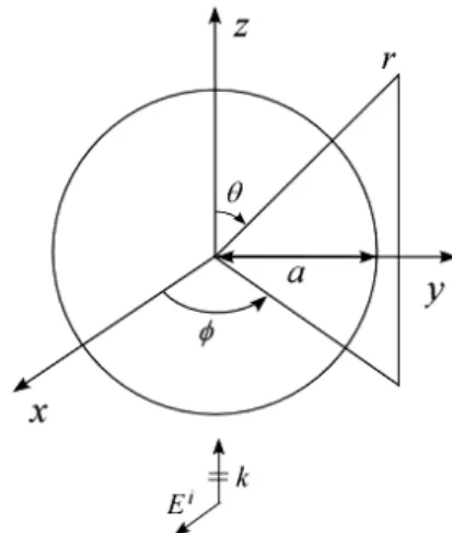
Consider a conducting sphere, embedded in homogeneous, unbounded free space, illuminated by an incident plane wave (Fig. 3.1). Taking the incident wave to be x-polarized and z-traveling yields:

cos 0 0 cos 0 0 i jkz jk r x i jkz jk r y E E e E e E E H e e θ θ η η − − − − = = = = (3.1)

The incident fields can be conveniently expressed as the sum of components that result Transverse Electric (TE) and Magnetic (TM) to r, that is, the magnetic and electric vector potentials Ar

 and Fr



that can be derived from Er



and Fr



respectively [52].

The r component of the incident field:

(

)

by expressing e jz in terms of spherical wave functions, (3.2) becomes:

0 0 cos (2 1) ( ) (cos ) i n r n n n E E j n j kr P jkr φ _θ θ ∞ − = ∂ = + ∂

∑

By applying relationships B kr_n( )=krb kr_n( )= πkr 2B_{n+1 2}(kr) and 1

n n P θ P ∂ ∂ = , we obtain: 1 0 2 0 cos (2 1) ( ) (cos ) ( ) i n r n n n E jE j n J kr P kr φ _θ θ ∞ − = ∂ = − + ∂

∑

Thanks to the form of (3.4), the magnetic vector potential can be constructed as:

1 0 1 cos ( ) (cos ) i r n n n n E A φ a J kr P θ ωµ ∞ = =

∑

A similar procedure using i r H and i r F gives: 1 0 1 sin ( ) (cos ) i r n n n n E F a J kr P k φ θ ∞ = =

∑

with an given by:

(2 1) ( 1) n n j n a n n − ₊ = + (3.7)

The scattered fields will be produced by an A_rand F_rof the same form as the incident field, with J replaced by n

( 2) n

H . Hence, the scattered potentials can be defined as:

(2) 1 0 1 cos ( ) (cos ) s r n n n n E A φ b H kr P θ ωµ ∞ = =

∑

∑

3.1. Scattering by an electrically small sphere and dipole moments 61

While the potential to be used to get the total fields, are:

(2) 1 0 1 cos ( ) ( ) (cos ) r n n n n n n E A φ a J kr b H kr P θ ωµ ∞ =   =

∑

∑

To satisfy boundary conditions E_θ =E_φ= at r = a, it is required: 0

(2) ( ) ( ) n n n n J ka b a H ka ′ = − ′ (3.10) (2) ( ) ( ) n n n n J ka c a H ka = − (3.11)

which completes the solution.

The distant scattered field can be derived from the general expressions by making use of the asymptotic expression:

(2) 1

( ) n jkr

n kr

H kr →_→∞ j +e− (3.12)

and retaining only the terms varying as 1/r. The result is:

1 1

0

1

(cos )

cos sin (cos )

sin s jkr n n n n n n jE P E e j b P c k r θ θ φ θ θ θ ∞ − =  _′  = _ − _  

∑

sin sin (cos )

sin s jkr n n n n n n jE P E e j b c P k r φ θ φ θ θ θ ∞ − =  _′  = _ − _  

∑

with the bn and cn given by (3.10), (3.11).

Being the back-scattered field defined as:

/ 2 s s s x E Eθθ π Eφθ π φ π== φ=−=π = = (3.14)

the echo area can be derived:

2 2 2 0 lim 4 s x e _r E A r E π →∞     = _{ }   (3.15)

By making use of the relationships: 1 (cos ) ( 1) ( 1) sin 2 n n P n n θ π θ θ → − → + (3.16) 1 ( 1) sin (cos ) ( 1) 2 n n P _{θ π} n n θ ′ θ _→ → − + (3.17)

The echo area can be simplified as:

2 (2) (2) 1 ( 1) (2 1) 4 ( ) ( ) n e n n n n A H ka H ka λ π ∞ = − + = ′

∑

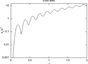
A plot of Ae/λ2 is shown in Fig. 3.2. For small ka, the n = 1 term of (3.18) becomes

dominant: 2 6 0 9 ( ) 4 e ka A λ ka π → → (3.19)

which is known as the Rayleigh scattering law and represents a good approximation when

a/λ < 0.1.

3.1.1. Dipole moments and scattering from a small conducting sphere 63

Expression (3.19) reveals that the echo area of small spheres varies as 1/λ4_{. For large}

spheres:

2

e ka

A →_→∞ πa (3.20)

which is the physical optics solution. The zone between the Rayleigh and optical approximations is known as the resonance region and is characterized by oscillations of the echo area.

\

3.1.1. Dipole moments and scattering from a small conducting sphere

Let us consider the process of scattering from a small conducting sphere having radius a, embedded in free space. A plane wave having its electric field polarized along the x-axis and traveling in the z-direction impinges on the sphere (Fig. 3.1). By using small argument expressions for the spherical Bessel functions, it can be found from (3.10), (3.11) and (3.7):

2 _{2 1} 0 0 1 1 2 ( 1)! ( ) (2 )! n n n ka n ka n n n ka b c n n j + → → +   + − →− _{→ }   (3.21)

thus the n = 1 terms of (3.13) dominate for small ka, being k the wavenumber in the medium. Hence, for the fields scattered in the far-field region it is obtained:

3 0 0 ( ) cos (cos 1/ 2) jkr s ka e E E k a kr θ φ θ − → → − (3.22(a)) 3 0 0 ( ) sin (1/ 2cos 1) jkr s ka e E E k a kr φ φ θ − → → − (3.22(b))

where E0 represents the magnitude of the incident electric field. A comparison of this result

with the radiation field of dipoles shows that the scattered field equals that of an x-directed electric dipole (Fig. 3.3):

3 0 2 4 ˆ ( ) x j Il xE ka k π η = (3.23)

plus the field of a y-directed magnetic dipole:

3 0 2 2 ˆ ( ) y Kl y E ka jk π = (3.24)

Figure 3.3. Bistatic radar cross section on the elevation plane of a PEC sphere whose diameter 2 a = 100 λ. Τhe scattered far-fields derived by employing the Mie series and a radiating electric dipole moment are compared.

The electric and magnetic dipole moments are originated from a surface current in the same direction on each side of the sphere and a circulating current respectively. For a conducting body the magnetic moment may vanish, while the electric moment must always exist. The expression for the θ component of the field produced by an x-directed electric dipole moment reads: 2 3 1 cos cos 4 jkr x Il j E e r r j r θ ωµ η _{φ θ} π ωε −   = _ + + _   (3.25)

In fact, the Mie series representation for the fields scattered by a small PEC sphere in the far-field region equals the far-fields produced by an electric dipole moment (Fig. 3.3).

As it is well-known, in the far-field any small body can be represented by a superposition of electric and magnetic dipole moments. However, what has not typically been handled in the past is the eventual accuracy of the dipole moment representations in the near-field region. This gap can be filled by recalling the Mie series representation of the scattering for the small sphere. Let us consider the dominant back-scattered field contribution:

1

(2) 1 (2)

0 1

(cos )

cos ( )sin (cos ) ( )

sin n n n n n n n E P E jb H kr P c H kr kr θ θ φ θ θ θ ∞ = ′  _{′ ′ ′}  = _ − _  

∑

H ′ ⋅ represents the derivative of the Henkel function [59] and bn, cn for small

3.1.1. Dipole moments and scattering from a small conducting sphere 65

By letting kr→0, by using the asymptotic expressions for the Henkel functions and its derivatives, and keeping only the n = 1 term it is obtained:

3 3 0cos cos 2 2 a ka E E j r r θ φ θ _{ }  =  _{ } +      (3.27)

In the limit a→0 and r→0, the (a/r)3 term dominates ka3/2r2, hence it is obtained:

3 0cos cos a E E r θ = φ θ      (3.28)

Regarding the dipole moment representation, substituting (3.23) in (3.25) it is obtained:

3 0 2 3 1 cos cos jkr jk a j E E e r r j r θ ωµ η _{φ θ} η ωε −   = _ + + _   (3.29)

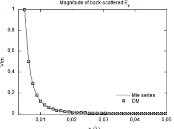
and keeping only the 1/r3 term yields the result in (3.28). Obviously, the Dipole Moment representation for the scattered fields remains valid in the near-field region, as can be noted in Fig. 3.4, where the back-scattered E_θ component produced by a x-directed electric dipole moment is compared with the Mie series result from the sphere’s surface to 0.05λ.

Figure 3.4. Back-scattered magnitude of the dominant Eθ component of a λ/200 radius PEC sphere as

a function of distance (from the sphere surface to 0,05λ). The Mie series and the dipole moment representations are compared.

3.1.2. Dipole moments and scattering from a small dielectric sphere

Consider a dielectric sphere of radius a and let the region r < a be characterized by ε1, µ1

and the region r > a by ε0, µ0. For this case, in addition to the previously derived total fields

produced by (3.9), there will be a field internal to the sphere, specified by the potentials:

1 0 1 1 0 cos ( ) (cos ) r n n n n E A φ d J k r P θ ωµ ∞ = =

∑

∑

The continuity of the tangential components of E and H:

t t t t E E H H + − + − = = (3.31)

must be met at r = a, superscripts – and + denoting the r < a and r > a regions respectively. By deriving the fields using (3.9) for the external region and (3.30) for the internal one and imposing the above described (3.31) boundary conditions, it is obtained:

1 0 0 1 0 1 0 1 (2) (2) 1 0 0 1 0 1 0 1 ( ) ( ) ( ) ( ) ( ) ( ) ( ) ( ) n n n n n n n n n n J k a J k a J k a J k a b a H k a J k a H k a J k a ε µ ε µ ε µ ε µ ′ ′ − + = ′ − ′ (3.32(a)) 1 0 0 1 0 1 0 1 (2) (2) 1 0 0 1 0 1 0 1 ( ) ( ) ( ) ( ) ( ) ( ) ( ) ( ) n n n n n n n n n n J k a J k a J k a J k a c a H k a J k a H k a J k a ε µ ε µ ε µ ε µ ′ ′ − + = ′ − ′ (3.32(b)) 1 0 (2) (2) 1 0 ( 0 ) ( 1 ) 0 1 ( 0 ) (1 ) n n n n n n j d a H k a J k a H k a J k a ε µ ε µ ε µ − = ′ − (3.32(c)) 0 1 (2) (2) 1 0 ( 0 ) (1 ) 0 1 ( 0 ) (1 ) n n n n n n j e a H k a J k a H k a J k a ε µ ε µ ε µ = ′ − ′ (3.32(d))

where an is given by (3.7). The conducting sphere case is obtained in the limit µ1→0, 1

ε → ∞.

In the case of an electrically small sphere the n = 1 coefficients dominate and reduce to:

0 3 1 0 0 1 ( ) 2 r k a r b k a ε ε → − →− + (3.33(a)) 0 3 1 0 0 1 ( ) 2 r k a r c k a µ µ → − →− + (3.33(b))

3.1.2. Dipole moments and scattering from a small dielectric sphere 67 0 1 0 9 2 (2 ) k a r r d jµ ε → → + (3.33(c)) 0 1 0 9 2 (2 ) k a r r e jε µ → → + (3.33(d))

where εr = ε1/ε0 and µr = µ1/µ0. This specialization is well-known as the quasi-static

solution. A calculation of the scattered fields reveals that it is the field produced by a x-directed electric dipole:

3 0 2 4 1 ( ) 2 r x r j Il E ka k π ε η ε − = + (3.34)

and a y-directed magnetic dipole:

3 0 2 4 1 ( ) 2 r x r j Kl E ka k π µ η µ − = + (3.35)

the magnetic dipole moment vanishing for non-magnetic dielectrics, while the electric dipole moment for magnetic materials with εr = 1. Again, these dipole moment representations

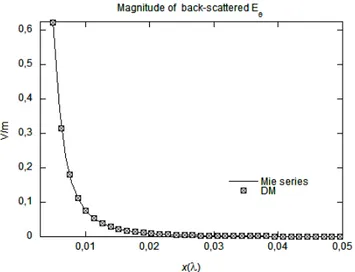
result valid both in the far- and in the near-field regions (see Figs. 3.5 and 3.6).

Figure 3.5. Bistatic radar cross section on the elevation plane of a dielectric (εr = 6) sphere whose

diameter 2 a = 100 λ0. Τhe scattered far-fields derived by employing the Mie series and a radiating

Figure 3.6. Back-scattered magnitude of the dominant Eθ component of a λ0/200 radius dielectric (εr = 6) sphere as a function of distance (from the sphere surface to 0,05λ0). The Mie series and the

dipole moment representations are compared.

Concluding, what has not been realized in the past and we have proved analytically, is that for a conducting or dielectric sphere whose radius is small, the dipole moment fields exactly match the original ones scattered by the sphere, all the way up to its surface.

3.2. The Dipole Moment Approach (DMA)

As we learned from the previous sections, when a sphere is illuminated by a plane wave of amplitude E0, the resulting scattered fields can be represented in terms of electric and

magnetic Dipole Moments (DMs). For the case of PEC spheres, they are expressed as:

3 0 2 4 ( ) E j Il E ka k π η = (3.36) 3 0 2 2 ( ) M Kl E ka jk π = (3.37)

while for dielectrics as:

3 0 2 4 1 ( ) 2 r E r j Il E ka k π ε η ε − = + (3.38) 3 0 2 4 1 ( ) 2 r M r j Kl E ka k π µ η µ − = + (3.39)

3.2. The Dipole Moment Approach (DMA) 69

Supposing a sphere is located at the origin, using the dipole moment representation for the scattered fields, for a z-oriented electric dipole moment the produced fields read:

2 3 1 cos 2 jkr r Il E e r j r η _θ π ωε −   =  +    (3.40) 2 3 1 sin 4 jkr Il j E e r r j r θ ωµ η _θ π ωε −   = _ + + _   (3.41)

In general, the scattering from a single PEC sphere can be represented by the field produced by a dipole moment whose orientation coincides with the polarization of the incident field. When formulating a problem that involves PEC objects, our first step is to represent the original scatterer by using a collection of perfectly conducting spheres. Next, we replace these spheres by their corresponding Dipole Moments and evaluate the generated electric fields.

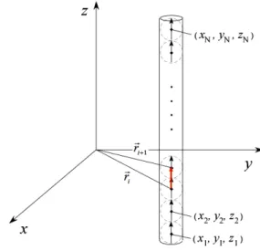
Obviously, for a PEC wire, each dipole moment will have a single preferred direction, representing the current path, matching the position of the adjacent sphere (Fig. 3.7). For a planar PEC structure as a sheet the associated preferred directions for the current flow will be those corresponding to the two adjacent spheres.

Figure 3.7. Dipole moments directions for a wire example.

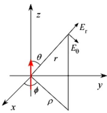
To evaluate the fields scattered by an arbitrarily oriented dipole moment at a given location, it is useful to work in Cartesian coordinates.

Figure 3.8. Spherical to Cartesian transformation for the fields scattered by a z-directed dipole moment.

By referring to Fig. 3.8, the z-component of the fields produced at observation point (xi, yi, zi) by a z-directed dipole moment centred at (xs, ys, zs) can be expressed as:

, cos sin

z z r

E =E θ−E_θ θ (3.42)

by rewriting (3.40) and (3.41) as:

2 3 2 3 1 cos cos 2 1 sin sin 4 jkr r r jkr Il E e e r j r Il j E e e r r j r θ θ η _{θ θ} π ωε ωµ η _{θ θ} π ωε − −   = _ + _ =     = _ + + _ =   (3.43) and being: cos / sin / z r r θ θ ρ = = (3.44) with 2 2 (x_i x_s) (y_i y_s) ρ= − + − , (3.42) becomes: 2 2 2 , 2 2 ( ) ( ) ( ) cos sin i s i s i s z z r r z z x x y y E e e e e r r θ θ θ θ − − + − = − = − (3.45) where r= (xi−xs)+(yi−ys)+(zi−zs).

3.2. The Dipole Moment Approach (DMA) 71

Following the same reasoning, and remembering that:

cos / sin / x y φ ρ φ ρ = = (3.46)

for the x- and y-directed contributions it is obtained:

2

( )( )

( ) cos sin cos ( ) ( ) i s i s

xz r r r z x z z x x E e e e e e e r r r θ θ θ ρ θ θ φ ρ − − = + = + = + (3.47) 2 ( )( )

( ) cos sin sin ( ) ( ) i s i s

yz r r r z y z z y y E e e e e e e r r r θ θ θ ρ θ θ φ ρ − − = + = + = + (3.48)

By properly rotating the reference system, the expressions for the fields scattered by an x-, y- and z-directed dipole moment in the three Cartesian directions can be obtained.

For x-directed dipole moments:

2 2 2 2 2 2 2 ( ) ( ) ( ) ( )( ) ( ) ( )( ) ( ) i s i s i s x x r t i s i s y x r t i s i s z x r t x x y y z z E e e r r x x y y E e e r x x z z E e e r − − + − = − − − = + − − = + (3.49)

for y-directed dipole moments:

2 2 2 2 2 2 2 ( )( ) ( ) ( ) ( ) ( ) ( )( ) ( ) i s i s x y r t i s i s i s y y r t i s i s z y r t x x y y E e e r y y x x z z E e e r r y y z z E e e r − − = + − − + − = − − − = + (3.50)

and for z-directed dipole moments:

2 2 2 2 2 2 2 ( )( ) ( ) ( )( ) ( ) ( ) ( ) ( ) i s i s x z r t i s i s y z r t i s i s i s z z r t x x z z E e e r y y z z E e e r z z x x y y E e e r r − − = + − − = + − − + − = − ...(3.51)

The above derived expressions can be adjusted in a matrix form as follows: x x x y x z i y x y y y z z x z y z z E E E Z E E E E E E     =       (3.52)

In simple matrix notation, the expressions for the fields scattered by a single sphere in an arbitrary u-direction can be written as:

T s T s

i

i i i i i i

u E⋅ =u E =Il u Z u (3.53)

with superscript T representing the transpose of column vector. It is worthwhile noticing that a preferred direction for the dipole moments can be specified for electrically connected clusters of spheres, while for single spheres it will be automatically given by the direction of the impinging wave.

For PEC structures we must impose the boundary condition that the total fields on the surface of the fictitious spheres must be zero:

s i u u

E = −E (3.53)

The fields scattered by a cluster of N spheres at some j-th locations on the PEC structure:

1 N s j i _ji i i E Il Z u = =

∑

To satisfy the boundary conditions at the N observation points (Fig. 3.9(a)):

1 N T scat T T inc j i ji j j j i j i u E u Il Z u u E = =

∑

this sets up a N×N matrix equation which is solved for the weight coefficients of the fields. The final Il’s can be derived by multiplying by 3 2

4 ( ) /

j π ka ηk .

This formulation relates to conventional Moment Method solution of the EFIE, in the sense that the string of fictitious spheres (dipole moments) which are used to represent the structure can be intended as ‘delta’ basis functions with amplitude given by (3.36). The resulting MoM system of equations is solved by ‘point matching’ the fields at given testing points (see Fig. 3.9(a)).

3.2. The Dipole Moment Approach (DMA) 73

(a) (b)

Figure 3.9. PEC rod: DM discretization with depicted dipole moments locations and points for applying the boundary conditions (a) and optimal discretization size ∆ for PEC structures (b).

By using a delta function representation it has been found, through testing convergence of the results (Figs. 3.10, 3.11), that the optimal discretization size ∆ = 0.5a for PEC structures, with

a having the physical meaning of the radius of the small discretizing sphere (Fig. 3.9(b)).

An analogue procedure can be carried out for the investigation of dielectrics. In fact, it has been already demonstrated that the scattering from a single dielectric sphere by using radiating dipole moments matches the Mie series solution up its surface (Fig. 3.6).

From the previous description we learn that there exists an unexploited way to model fine structures, the procedure consisting in first replacing fine structures with strings of spheres, then in turn replace them with unknown dipole moments. The MoM can be then deployed to solve for the weight coefficients of the fields to derive the unknown dipole moments.

It is useful to recognize that the dipole moment specified previously (3.34, 3.35) is an equivalent condensed representation. But, since we are dealing with dielectric materials where the fields do exist inside the sphere, unlike PECs, it is necessary to derive an equivalent volume representation of it.

The easiest way of doing that is to assume the final distributed moment to be a constant times the condensed value. This constant F, will be denoted as the Consistency Factor.

This factor can be derived, by considering a single sphere located at (x0, y0, z0), matching the

polarization currents: 0( 1) i s r E E FIl ε ε − _ +  _=  (3.56) where inc ₀

E =E represents the incident electric field at (x0, y0, z0) and the condensed electric

For small spheres, (i.e. ka→0), the fields scattered by the electric moment reduce to: 2 3 3 1 1 sin 4 2 4 s Il jka j Il E e a a j a j a ωµ η π π ωε π ωε −     = −  + +  ≈ −       (3.57)

by substituting (3.57) into (3.56) it is obtained:

3 3 4 j F a πω − ≈ (3.58)

Note that in the above representation we have matched the polarization currents because the quantities we are dealing with are volume distributed. This condition is termed as

Consistency Condition. It is important to underline that the scattered field is calculated at the

surface of the sphere and pretend as it would be the same at the centre. This argument is valid if the sphere is small, so that there is no room for field variations inside.

The Method of Moments (MoM) is then deployed to build a matrix equation to be solved. Clearly, by applying condition (3.57) as pictorially described in Fig. 3.10(b), the singularity issue plaguing the conventional MoM formulation is naturally overcome.

(a) (b)

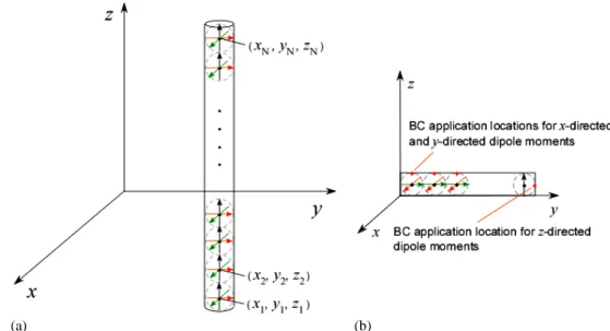
Figure 3.10. Dielectric rod discretization through x-, y- and z-directed DMs depicted dipole moments (a) and points for boundary conditions application (b).

3.2. The Dipole Moment Approach (DMA) 75

While formulating the problem, we assume consistency factor F to be the same, irrespective of whether the sphere is independent or in a cluster. Let’s consider a rod oriented along z extending from l/2 to l/2 and of thickness d. We then replace the rod by a string of N spheres of diameter d = 2a.

In the case of dielectric structures, the spheres are replaced with three equivalent independent dipole moments, one along each direction (Fig. 3.10(a)). The rest of the formulation goes as follows:

• Let n s

FIl be the effective dipole moment relating to nth sphere, directed along ˆs. • Let ,

n s inc

E be the incident field component at the centre of nth sphere, along ˆs. • nm_,

t s

E represents the scattered field component along ˆt on nth sphere because of ˆs−

oriented dipole of mth sphere, namely m s

FIl .

A matrix equation is formed by applying the Consistency Condition at centre of each sphere, for each component. For ˆx− directed dipole moment of n = 1, i.e. for all contributions on first sphere, we get:

1 11 12 1 11 12 1 11 12 1 1

0( 1) , ... ... ..

N N N

r Ex inc Exx Exx Exx Exy Exy Exy Exz Exz Exz FIlx

ε ε − _ + + + + + + + + + + + + _= (3.59)

Repeating the procedure on the other spheres up to the Nth, for it we get:

1 2 1 2 1 2

0( 1) , ... ... ..

N N N NN N N NN N N NN N

r Ex inc Exx Exx Exx Exy Exy Exy Exz Exz Exz FIlx

ε ε − _ + + + + + + + + + + + + _= (3.60)

Similarly, for ˆy−directed dipole moment of n = 1, namely considering all contributions on

1st sphere, we get: 1 11 12 1 11 12 1 11 12 1 1 0( 1) , ... ... .. N N N r Ey inc Eyx Eyx Eyx Eyy Eyy Eyy Eyz Eyz Eyz FIly ε ε − _ + + + + + + + + + + + + _= (3.61)

Repeating the procedure on the other spheres up to the Nth , for it we get:

1 2 1 2 1 2

0( 1) , ... ... ..

N N N NN N N NN N N NN N

r Ey inc Eyx Eyx Eyx Eyy Eyy Eyy Eyz Eyz Eyz FIly

ε ε − _ + + + + + + + + + + + + _= (3.62)

Similarly, for ˆz−directed dipole moment of n = 1, i.e. considering all contributions on 1st sphere, we get: 1 11 12 1 11 12 1 11 12 1 1 0( 1) , ... ... .. N N N r Ez inc Ezx Ezx Ezx Ezy Ezy Ezy Ezz Ezz Ezz FIlz ε ε − _ + + + + + + + + + + + + _= (3.63)

By repeating the procedure for the other spheres up to n = N, on Nth sphere it is obtained: 1 2 1 2 1 2 0( 1) , ... ... .. N N N NN N N NN N N NN N r Ez inc Ezx Ezx Ezx Ezy Ezy Ezy Ezz Ezz Ezz FIlz ε ε − _ + + + + + + + + + + + + _= (3.64)

The system can be put in matrix form as:

[ ] [

]

[ ]

[ ]

[ ] [

]

where i-th sub-block

[ ]

1 0 1 0 1 i FIl               (3.66)

It is crucial to underline that the self terms in these equations, namely ,

nn t s

E are computed in the surface, instead of centre, in turn getting rid of singularity.

From the above formulation we get 3N variables and 3N equations. It is solved for the E’s and the Il’s are derived by multiplying by 3 2

4 ( ) ( r 1) / ( r 2)

j π ka ε − ηk ε + . After having solved the equations for the relative weight coefficients, the Il’s can be used to calculated the produced fields.

When the MoM system of equations is solved by ‘point matching’ the fields at given testing locations (see Fig. 3.10(b)), it can be noted that the discretization size ∆(a), with a having the physical meaning of the radius of the small discretizing dielectric sphere, depends upon the dielectric parameters of the structure.

3.3. The Characteristic Basis Function Method (CBFM) applied to the DMA 77

3.3. The Characteristic Basis Function Method (CBFM) applied to the

Dipole Moment Approach (DMA)

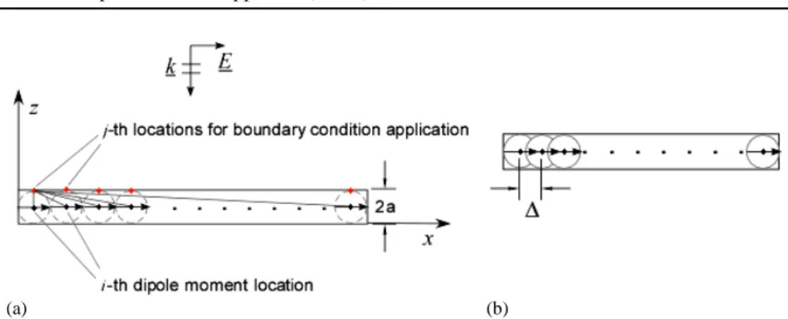
The proposed method though it is accurate and captures all the physics overcoming some of the issues associated with the conventional MoM technique, is not the most efficient from numerical point of view [60]. This is because the number of spheres used to represent a three-dimensional object can grow very rapidly if the diameter of the meshing spherical building block is small, as is often the case.

For instance, for a thin-wire scatterer (see Fig. 3.10), the diameter of the spheres used to represent it is the same as that of the wire. The number of unknowns can be significantly reduced, however, so as to make it comparable to that used in the conventional MoM formulation, via the use of macro-basis functions. We have shown that it is relatively easy to choose these macro basis functions, and that the fields generated by these functions can be conveniently expressed in closed-form. We can further improve the computational efficiency of the method by using techniques such as the CBFM [37].

3.3.1. CBFM basic theory

Let us now consider a generic 3-D object for which the application of the conventional MoM formulation, based on a sub-sectional basis functions, to some Integral Equation (IE), leads to a dense linear system of the form:

Z J⋅ =V (3.67)

where Z is the generalized N MoM × N MoM impedance matrix, J and V are N MoM × 1 vectors, being N MoM the number of unknowns. For large problems, the matrix system (3.67) can be used to solve for thousands of unknowns, this posing a burden on the computer memory and CPU time.

Furthermore, the size of the MoM impedance matrix becomes prohibitive for direct solvers when N MoM is large, requiring to employ iterative solvers. However, the latter suffer from convergence difficulties when (3.67) is ill-conditioned, and, moreover, they require solving the system anew for each excitation.

The use of macro-domain basis functions leads to a ‘reduced’ matrix that results much smaller than that built via the original MoM and can be solved directly, without requiring preconditioners. Moreover, multiple right hand sides can be handled efficiently.

The CBFM technique can be summarized in the following basic steps:

i The structure to be analyzed is partitioned into a number M of small domains, called ‘blocks’ (see Fig. 3.15).

ii A set of NPW Characteristic Basis Functions (CBFs) is built for each block by exciting it with Plane Wave excitations (PWs) incident from NPW angles (the number NPW of excitations is deliberately overestimated to capture all the present Degrees Of Freedom for the problem at hand).

iii In order to compute the CBFs all blocks are extended by a fixed amount Δ (tipically

0.2λ to 0.4λ) in all directions with the exception of free edges, to avoid a singular behavior for the current distribution within the original block introduced by the truncation that creates fictitious edges.

iv The redundant information is eliminated via the use of the Singular Value

Decomposition (SVD) procedure through which only K M× basis functions (K<

NPW) are retained, K for each of the M blocks).

v A KM×KM reduced system matrix is solved for KM complex unknowns.

vi The solution to the entire problem is finally expressed by a linear combination of

the CBFs weighted by the α (KM) coefficients.

Figure 3.11. Geometry of a plate partitioned into 9 blocks. Extended blocks are represented in orange lines.

3.3.1. CBFM basic theory 79

After the geometry of the object to be analyzed is partitioned into a number of blocks, each of those is characterized in isolation through the so-called primary Characteristic Basis Functions (CBFs). The CBFs represent a redundant collection of localized solutions which also account for the interactions with the remaining blocks. The upper limit on the size of the blocks is bounded by the available RAM needed to solve the single block.

Next a set of NPW CBFs are constructed for each block by illuminating it by multiple plane wave excitations (PWS) incident at NPW angles (Fig. 3.12).

Figure 3.12. A number of plane wave excitations incident on i-th block.

A number NPW of CBFs are derived for each block by solving the linear system of equations:

ext CBFs PWs ii iN N Z ⋅J =V (3.68) where CBFs iN J is the Nth CBF of block i (i = 1,..,M), PWS N

V is the excitation vector of the relative CBF, ext

ii

Z is the interaction matrix of the extended block extracted from the original MoM matrix.

The system is solved N times for each block; next, the CBFs are truncated by discarding the current weight coefficients belonging to the extension region. The result is a number N of redundant current solution vectors Ji for each block.

In order to reduce the redundancy of the previously derived collection of CBFs, each Ji

[ F×N ] matrix is factored by using the Singular Value Decomposition (SVD). The procedure extracts the most linear independent columns of the Ji matrices.

In fact, each Ji matrix can be written as the product of three matrices:

J= ΣU V (3.69)

where U is a K× matrix, V is a K N×Nmatrix and Σ is a K×N diagonal matrix.

The singular values matrix Σ is normalized to its maximum, then only the singular values (in number K < N) above a certain threshold (typically 10-2) are retained, while the others are set to zero getting ′Σ .

A non-redundant set of CBFs (in number = K) is obtained for each block, through:

i

J′= Σ U ′ (3.70)

where ′Σ is the modified singular values matrix:

1 0 0 0 0 0 0 0 0 0 0 0 0 K λ λ         ′ Σ =              (3.71)

and λi are the retained singular values.

The solution to the complete problem will be then expressed as a weighted linear combination of the CBFs:

[ ]

[ ]

[ ]

[ ]

[ ]

[ ]

[ ]

∑

∑

∑

where α are the unknown expansion coefficients, ( )i k

J is kth CBF of block i and x is the solution to the original system of equations Ax=b.

The expansion coefficients α are solution to the reduced matrix system:

[ ]

whose Right Hand Side (RHS) (excitation) vector is defined as:

1 , 1 , H inc H inc M M J E v J E     =          (3.74)

3.3.2. The CBFM applied to the DMA 81

3.3.2. The CBFM applied to the DMA

For the sake of illustrating the application of the CBFM to the DMA, we consider a thin dielectric (εr = 6) sheet whose thickness is λ/100 at the operating frequency of 1 GHz and it

is 0.162λ on the side. The thin sheet is divided into 4 blocks, as reported shown in Figure 3.13. Although generally the blocks can have different sizes, we assume that they have approximately the same dimension Nu in terms of unknowns.

(a) (b)

Figure 3.13. Plate structure partitioned into 4 blocks. The unknowns highlighted in light blue represent those constituting the block, while those in red represent the blocks’ extensions. The blocks and related extensions are shown for (a) external and (b) internal block cases.

In order to compute the CBFs, the blocks are extended of an amount proportional to the dimension of the discretizing sphere (see Fig. 3.13), as opposed to conventional CBFM in which the extension has to range from 0.2λ to 0.4λ.

Then, to mitigate the truncation effect, we impose the coefficients relative to the extensions to obey specific relations. For example we want the coefficients of the extension of block 1 (see Fig. 3.13(a)) to fulfil the following relations:

101 121 141 381 102 122 142 382 120 140 160 400 α α α α α α α α α α α α = = = = = = = = = = = =     (3.75)

which, in turn, reflects on elements of sub-matrix of 1st block extracted from the original MoM matrix as:

,101 ,101 ,121 ,141 ,381 ,102 ,102 ,122 ,142 ,382 ,120 ,120 ,140 ,160 ,400 k k k k k k k k k k k k k k k E E E E E E E E E E E E E E E = + + + + = + + + + = + + + +     (3.76)

where Ek h, represents the field produced on element k from dipole moment h. The

self-impedance matrix is then employed to generate the NPW CBFs induced on a given block by exciting it with a set of windowed plane wave excitations impinging upon the object with two different polarizations varying the incident angle.

For the present example, we employed TE and TM polarized incident waves varying the incident angle (θi = 30i, i = 0, 1, ..,11) for a total of 24 different excitations.

Figure 3.14. A number of plane wave excitations incident on i-th block.

Then, the system constituted by the interaction matrix of i-th extended block extracted from the original MoM matrix is solved anew for each of the 24 excitations, getting a set of 24 CBFs for each block. At this time, the CBFs are truncated by discarding the current weight coefficients belonging to the extension region.

The Singular Value Decomposition (SVD) is applied to each set of CBFs to reduce their redundancy. Each Ji matrix (which at the moment is a 300x24 matrix) is decomposed as in

(3.69) and a threshold of 10-2 is chosen for the problem at hand (a plot of the normalized singular values is reported in Fig. 3.15).

Only the first 6 singular values exceed the selected threshold, so the remaining ones are set to zero in matrix Σ. The most linear independent localized current solutions are derived, through (3.70), for each block.

3.3.2. The CBFM applied to the DMA 83

Figure 3.15. Normalized singular values for CBFs of all blocks (a similar behavior can be observed for blocks 1 and 4 and blocks 2 and 3 due to symmetry). Only the first 6 singular values result to be over the set threshold for all blocks.

(a) (b)

(c) (d)

Figure 3.16. Amplitude variation of the x-component of CBFs 1 (a), 3(b), 5(c) and 6(d) on the entire structure. The bottom regions highlighted in yellow, green, blue and pink represent the blocks in which the structure has been partitioned.

The reduced matrix system is built through (3.73), solved for normal incidence and compared with pure DM solution and conventional MoM approach. The x- and y- components of the current are compared with pure DM in Fig. 3.17, while the magnitude of the dominant back-scattered near field component and the RCS are compared in Fig. 3.18.

(a) (b)

(c) (d)

Figure 3.17. Amplitude variation of Jx derived through pure DMA (a) and DMCBFM (b) and of Jy

derived through pure DMA (c) and DMCBFM (d).

(a) (b)

Figure 3.18. Pure DM – DMCBFM-conventional MoM comparisons of backscattered Ex from λ/10 to

3.3.2. The CBFM applied to the DMA 85

Through (3.73) the original system that should have been solved for 1200 unknowns is reduced to a more manageable 24 unknowns problem. Moreover, it has to be pointed out that the final reduced matrix is independent of the excitation, enabling us to analyze a problem involving multiple excitations by solving the reduced system for a new r.h.s..

The reduced matrix can be stored on a hard drive and reused whenever needed to analyze for a new excitation. Furthermore, if the geometry within a particular block is modified, only the CBFs relative to that particular block needs to be recomputed.

The CBFM technique realizes a saving in the CPU running time and Random Access Memory (RAM) requirement with respect to a conventional MoM technique. The memory requirement is now proportional to the square of the self-impedance matrix of an extended block, opposed to conventional MoM where the storage requirement is related to the square of the dimension of the entire impedance matrix [61].

Through the particular truncation technique described in (3.75), an additional advantage is introduced in terms of memory and time without affecting the accuracy of the method (Fig. 3.18 (a, b)).

3.4. Numerical results

In the following section some numerical experiments demonstrating the accuracy as well as the flexibility of the method in the context of solving scattering problems will be presented. Both PEC and dielectric scatterers will be taken as test examples while both the near- and far-field distributions will be derived to test the accuracy of the method.

In particular, the optimum spacing ∆ between the constituent dipole moments will be studied both for PEC and dielectrics in the context of matching the current distribution and the scattered fields.

The same discretizing step will be demonstrated to work equally well, irrespective of the geometry of the scatterer.

3.4.1. λ/4 in length λ/100 in diameter conducting wire

Consider as a test example a PEC rod extending along the z-axis, measuring λ/4 in length (at the operating frequency of 1 GHz) and being λ/100 thick. The wire is invested by a –x-traveling plane wave whose E-field is polarized along z.

In Fig. 3.19 the magnitude (a) and phase (b) distributions of the current along the wire are presented while Fig. 3.20 shows the backscattered Ez. Both results are presented as a function

of the distance ∆ between the discretizing spheres.

(a) (b)

Figure 3.19. Magnitude (a) and Phase (b) distributions of Jz along a λ/4 in length PEC rod. The

discretization ∆ is varied from 2a to 0.5a until convergence is achieved.

As we can conclude experimentally, a discretizing step ∆ = 0.5a is optimum for the analysis of problems involving PEC structures.

3.4.2. λ/2 in length λ/100 in diameter conducting bend wire 87

(a) (b)

Figure 3.20 Magnitude (a) and Phase (b) distributions of backscattered Ez from the rod surface to 0.2λ.

The discretization ∆ is varied from 2a to 0.5a until convergence is achieved.

3.4.2. λ/2 in length λ/100 in diameter conducting bend-wire

Let us consider a conducting bend-wire whose total length is λ/2 and whose diameter is λ/100 which extends on the xy-plane at z = 0 (Fig. 3.21). A plane wave traveling along -y at the operating frequency of 1 GHz impinges on the bend structure, its E-field is polarized in the direction θ = π/4, φ = 0.

The discretization step for the structure is kept same as in the previous example, while the magnitude and phase distributions of the current are calculated along the two branches of the wire (Fig. 3.22). The magnitude and phase distributions of the x- and y- components of the back-scattered E-field are derived along the y-axis from λ/10 to 2λ (Figs. 3.23 and 3.24).

Figure 3.21. PEC bend wire geometry, λ/2 in length. A θ = π/2, φ = 0 polarized E-field impinges on the structure while the output field is observed along y from λ/10 to 2λ.

(a) (b)

Figure 3.22. Magnitude (a) and Phase (b) distributions of J alog a λ/2 in length PEC bend wire. The DM and conventional MoM results are compared.

(a) (b)

Figure 3.23 Magnitude (a) and Phase (b) distributions of backscattered Ex (same as Ez) from

λ/10 to 2λ along the y-axis. The results derived through the DMA are compared against the conventional MoM.

3.4.3. λ/4 on the side, λ/100 in length square dielectric plate 89

(a) (b)

Figure 3.24 Magnitude (a) and Phase (b) distributions of backscattered Ey from λ/10 to 2λ along the

y-axis. The results derived through the DMA are compared against the conventional MoM.

3.4.3. λ/4 on the side, λ/100 in length square dielectric plate

Let us consider as a test example a dielectric (εr = 6) plate which extends on the xy-plane, at

z = 0, λ/4 on the side (at the operating frequency of 1 GHz) and λ/100 thick. A plane wave

which propagates along z with its E-field polarized along x is incident upon the structure. The magnitude (a) and phase (b) distributions of the backscattered dominant component Ex

as a function of the distance ∆ between the discretizing spheres is presented in Fig. 3.25.

(a) (b)

Figure 3.25 Magnitude distributions of x- (a) and y- (b) components of the current on the plate. ∆ = 1.6a has been used to get there results.

(a) (b)

Figure 3.26 Magnitude (a) and Phase (b) distributions of backscattered Ex from λ/10 to λ/2 as a

function of the spacing ∆ between the discretizing dipole moments.

As emerges from Fig. 3.26, a discretizing step ∆ = 1.6a is optimum for the analysis of problems involving dielectrics with relative dielectric constant equal to 6.

3.4.4. Dielectric sphere

λ/20 in radius

Let us consider as a test example a dielectric (εr = 6) sphere whose radius is λ/20, invested

by a plane wave whose electric field is polarized along x.

The backscattered dominant component from the surface of the sphere to λ/2 has been derived and compared with Mie series.

(a) (b)

Figure 3.27 Magnitude (a) and phase (b) distributions of backscattered Eθ from the sphere's surface to

λ/2 with spacing ∆ between the discretizing dipole moments equal to 1.6a. The results derived through the DMA are compared with those obtained by using the Mie series representation.

3.4.5. Dielectric coated conducting plate 91

To prove that the spacing derived for dielectrics with εr = 6 works equally well irrespective

of the analyzed geometry, the sphere has been analyzed as a cluster of small spheres (dipole moments) with relative spacing ∆ = 1.6a, with a = λ/200.

As can be noted from Figs. 3.26 and 3.27, the same discretizing step yield accurate results irrespective of the geometry under analysis. In fact, the fields scattered by a dielectric sphere with same dielectric constant of the plate matches the Mie series result up to its surface.

3.4.5. Dielectric coated conducting plate

Let us consider as an example of composite structure, a dielectric (εr = 6) coated conducting

plate which measures λ/10 in length and is 3λ/100 thick (see Fig. 3.28). The structure is invested by a plane wave traveling along the –z direction with E-field polarized along x. The previously discussed discretizations are used to model the PEC and dielectric parts of the composite structure.

The backscattered near fields as well as the bistatic RCS are reported in Figs. 3.29 and 3.30.

Figure 3.28. PEC plate coated with εr = 6 dielectric.

(a) (b)

Figure 3.29 Magnitude (a) and phase (b) distributions of backscattered Ex from 2 to 3λ along the

Figure 3.30 Bistatic RCS on the elevation plane (φ = 0) for a dielectric coated PEC plate at normal incidence.