Chapter 4
Results and Discussions
4.1 Comparison of power number and power consumption for
the two flow configurations
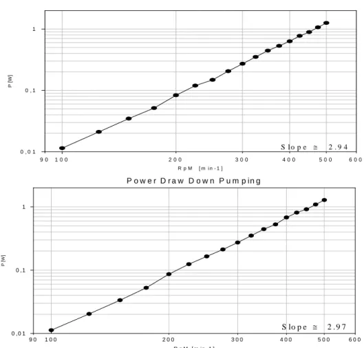
The investigation on the energy input passed through the measurement of the power number for the two impellers. The first check on the reliability of the results is obtained plotting on a double logarithmic scale, the experimental power data, which according to Nienow et al. (1994), it should give a slope of 3. Figure 4.1, shows the measured Power versus N for both the Up-pumping and the Down-pumping configurations.
P o w e r D r a w D o w n P u m p in g R p M [ m in - 1 ] 9 0 1 0 0 2 0 0 3 0 0 4 0 0 5 0 0 6 0 0 P [W ] 0 , 0 1 0 , 1 1 S lo p e ≅ 2 . 9 7 P o w e r D r a w U p P u m p i n g R p M [ m i n - 1 ] 9 0 1 0 0 2 0 0 3 0 0 4 0 0 5 0 0 6 0 0 P [W ] 0 , 0 1 0 , 1 1 S l o p e ≅ 2 . 9 4
The slopes obtained are in good accordance with the theory, and therefore we can consider the following results on NPo and εT reliable.
A similar NPo for both the impellers is expected. NPo as seen in the previous chapters depends strongly on the geometry of the impeller; different values might be attributed to slight geometrical differences. In the next graphs (Figure 4.2) the NPo of the two impellers are compared. RpM [min-1] 100 200 300 400 500 NPo 0,0 0,5 1,0 1,5 2,0 2,5
Down Pumping Configuration
RpM [min-1] 100 200 300 400 500 NPo 0,0 0,5 1,0 1,5 2,0 2,5 Up Pumping Configuration Mean value: 1.567 Mean value: 1.594 NPo (300 RpM) = 1.558 NPo (300 RpM) = 1.551
Figure 4.2 Power Number profile at variable RpM
Practically identical power numbers, suggest that the geometries, and symmetries of both the impellers are very similar and moreover, that the vessel configuration (i.e. clearance) does not disturb the flow.
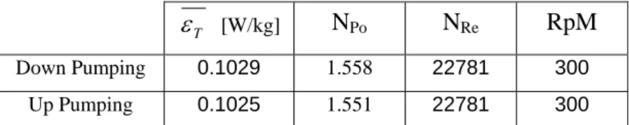
For this reason all of the following experimental PIV measures have been carried out, at the same speed. In the table below the average power characteristics are summarized.
T
ε [W/kg] NPo NRe RpM
Down Pumping 0.1029 1.558 22781 300 Up Pumping 0.1025 1.551 22781 300
4.2 Power characteristics and time-averaged flow field for a PBT in
up-pumping and down pumping configurations
The time averaged analysis was obtained, as described in the chapter 3 from 500 instantaneous flow fields (1000 frames). Fluctuations in the velocity that can be seen comparing different instantaneous images of the flow are averaged out in the time average (H.S. Yoon et al., 2001).
4.2.1 Time averaged flow field and instantaneous flow profiles
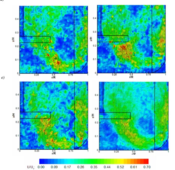
In the following images the difference between the instantaneous capture and the mean values near the impeller for the down pumping configuration are highlighted.
a) b)
c)
d)
Captures were taken at random impeller position, in order to state that the mean velocity field was actually time averaged.
Is evident from figure 4.3 how the instantaneous fluctuations present in a), b) and c), are smoothed out in the mean flow field and the main flow recirculation is clear. The similar results were obtained in the up pumping configuration, thus the same observations are possible.
4.2.2 Comparison between time averaged flow field configurations
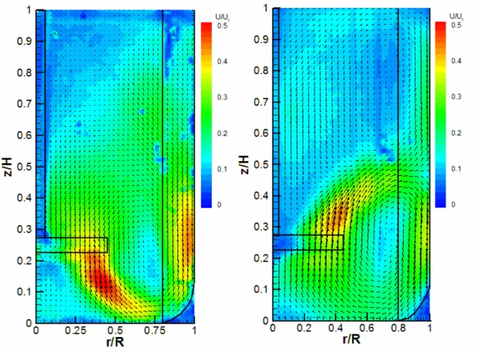
In the following graphs the time-average flow fields are compared. The structures of the two flow configurations are evident.
Figure 4.4: Time average flow field. Down pumping on the left and Up pumping on the right.
In figure 4.4 is clear how the two flow fields generated from the two flow configurations differ from each other. Only one wide recirculation loop is observed in the down wards configuration, while in the other mode, the discharge stream from the impeller creates two main vortex loops. The velocities are in both cases similar and for down pumping the maximum velocity normalized by the blade tip speed is 0.51, while for up pumping is 0.48.
4.2.3 Dissipation of turbulent kinetic energy
The turbulent kinetic energy is calculated as described in the previous chapter, with Eq.
2.13. The levels of turbulent kinetic energy differ between the two configurations.
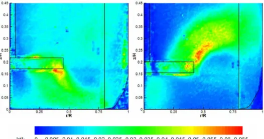
The values of the turbulent kinetic energy, from now on, will be reported in every figure, normalized by utip2. Thus kt*=kt/ utip2.
Figure 4.5: Turbulent kinetic energy in time averaged configuration
The information reported in Figure 4.5, describe an overall high value of turbulent kinetic energy in the down pumping configuration, and a more localized area of high turbulent kinetic energy in the up pumping mode. The kt* values outside the zone directly interested by the discharge jet, in the up pumping configuration, reach for z/H=0.35 and r/R= 0.2 kt*=0.005; half of the value recorded in the other configuration, for the same coordinates.
At the same time is evident how the area with kt* grater than 0.05 is more extended in the up-pumping configuration.
The integral of the values of the kt* over the volume of the vessel for both the flow configurations, must tend to the same value, which isεT , chosen to be 0.1 [W/kg]. This has been done in the 4.3.6 paragraph on the energy evaluation comparison.
4.2.4 Energy dissipations rates evaluated through dimensional analysis
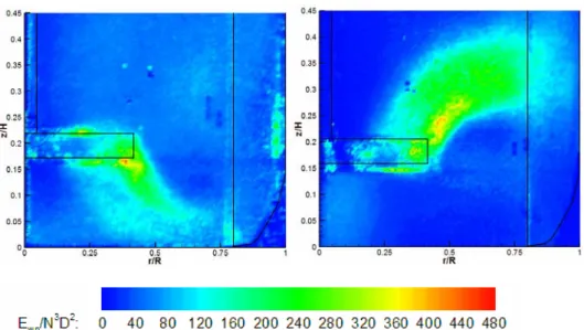
In the analysis of the dissipation rates of the turbulent energy, the same energy distribution pattern is observed because a constant integral length scale has been adopted (D/10).
Figure 4.6: Time averaged turbulent kinetic energy dissipation rate evaluated with dimensional analysis.
Also in this case are valid the same considerations done for the kt* distribution. The discharge zone near the impeller, in the up pumping configuration, has a larger zone where Ewp/N3D2 exceeds 300. For z/H=0.35 and r/R= 0.2, the Ewp/N3D2 valuein the up pumping configuration is 9.98, while in the down pumping is 48.8.
4.2.5 Direct calculation from the definition
Appling this method to the evaluation of the turbulent kinetic energy wants to provide with a mean of comparison of the above results and to separate the measure of the energy dissipation from the measure of kt*. From Figure 4.7, the area where the maximum values of the energy dissipation rate are present and their extension result very clear, with clearly an advantage in terms of dissipation rate, for the up pumping configuration. The color scale chosen to highlight the propriety described in the previous lines, hides the characteristic higher values of Eb/N3D2 in the areas not directly interested by the discharge jet.
Figure 4.7: Time averaged turbulent kinetic energy dissipation rate evaluated from the direct calculation from the
definition.
For the same coordinates investigated before, the results for the two flow configurations are the following. For r/R=0.2 and z/H=0.35, Eb/N3D2down= 5X10⁻⁵, while for Eb/N3D2up=3.6 X10-5.
4.2.6 Large eddy PIV method
In Figure 4.8 is shown the results of the application of the large eddy PIV method over the time average flow field. The values of Esgs/N3D2 higher than 0.02, define the area where the dissipation rate is the highest.
Later in the paragraph related to the angle resolved analysis, a more exhaustive overview on the three methods adopted has been proposed, in order to explain the necessity to estimate the energy dissipation rate with different approaches. Moreover, a mathematical approach has been done, evaluating the integral over the volume for each method of the energy dissipated, and compared with the total energy input. Every aspect has been described in the following pages.
4.2.7 Vorticity
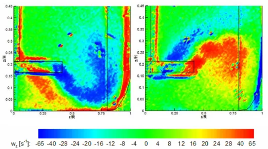
The vorticity described in Figure 4.9, for the time averaged analysis, shows not only the rotational direction of the vortex, but also the intensity.
Figure 4.9: Time averaged Vorticity in the two flow configuration.
From Figure 4.9 is evident how the flow structures and the main vortex rotational direction are different.
In the down pumping configuration, is evident a secondary loop beneath the impeller rotating clockwise, with maximum intensity of 53 s-1, while the intensity of the main recirculation loop near the impeller -110 s-1.
The up pumping discharge jet from the impeller breaks into two streams; one part forms the main recirculation loop, while the second one is responsible for the upper loop. The main recirculation loop in the up pumping configuration, has a maximum intensity of 120 s-1, and the rotation is clockwise. The upper recirculation loop starts from the impeller and is there that has the maximum intensity, measured to be 56 s-1.
4.2.8 Flow number evaluation
The flow number (NQ) is a dimensionless number of the pumping capacity of the impeller
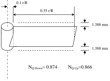
Eq .2.9. The area adopted for the measurement of the NQ is described in Figure 4.10.
0.35 r/R 1.388 mm 1.388 mm 0.1 r/R NQ Up=0.866 NQ Down= 0.874
Figure 4.10: Schematic representation of the coordinates taken to evaluate NQ
The power numbers calculated are very similar, as expected. The value of 0.87 is in good agreement with the values previously measured in other works, 0.88 for a 6-blade PBT (Hockey and Nouri, 1996).
A distance of 1.388 mm from the blade was chosen after analyzing the flow field, in order to measure the fully developed flow without taking in account the entrained flow, as discussed in the second chapter.
4.3 Angle resolved PIV measurements for a PBT impeller in
up-pumping and down-pumping configurations
As shown in this paragraph, the angle resolved measurement gives a more detailed and complete understanding of the flow configuration in a particular plane of interest. Triggering the blade passage reduces the noise due to the macro velocity fluctuation, as blade passage, which can be identified in the time average measurement, from any energy spectrum analysis, or a frequency analysis (Yianneskis et al., 1987). The result is an instantaneous capture of the flow around the impeller at different angles but always in the same PIV-plane in the vicinity of the baffle. The angle resolved measure, allows the decomposition of the information given by the time averaged, focusing on the periodicity of the blade passage.
4.3.1 Angle resolved flow field
The flow field around the impeller is function of the angle respect to the blade. The 0°
angle is taken for the laser crossing the blade of the impeller in the middle. Figure 4.10 shows the average flow field over 500 captures, measured at different blade angles.
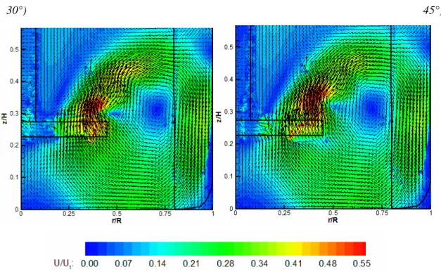
30°) 45°)
Figure 4.10: Up pumping flow field at different angles
The flow around the impeller has a periodicity of 1/6 of the impeller revolution, as observed in Figure 4.10. The area in which the maximum velocity is present, moves further away from the blade, as the angle increases.
In the first image, for 0° angle, an elongation of the area where the velocity is higher than 0.44 U/Utip, breaks up in the following image for 15°, in two. The zone further away from the impeller reduces its velocity as it goes further; bringing new energy to the point where the flow splits to form the primary and the secondary loop.
The same pattern is observed in the down pumping configuration. As shown from the flow field in Figure 4.10.
0°) 15°)
30°) 45°)
Figure 4.11: Down pumping flow field at different angles
In the discharge region near the impeller, it is found the maximum normalized velocity. Clearly its value varies with the blade position. With the dataset available on the two flow configuration, the two periodicities can be further analyzed. From the information observed comparing Figure 4.10 and Figure 4.11, is evident how the periodicity of the blade movement is the same whether the configuration of the flow is up pumping or down. Observing the 0° angle of both configurations, the area where the velocity is above 0.5 U/Ut, is on the impeller and relative distance from the blade increases in the same way for both set-ups. For 30° angle a clear break up in the discharge jet is visible in both, up and down pumping set-ups. These flow similarities are observed for every angle.
The flow induced by the impeller in the main loop, maintains constant characteristics varying the blade angle. These flow patterns will be further discussed in the following paragraphs.
4.3.2 Turbulent kinetic energy
The angle resolved study of the turbulent kinetic energy, is shown in the following figures.
Figure 4.12 shows the turbulent kinetic contours for four blade positions.
0°) 15°)
30°) 45°)
Figure 4.12: Down pumping turbulent kinetic energy
In the above figure, for a 0 degrees angle, the area interested by the maximum kinetic energy is generated by the passage of the previous blade. This explains why, for some angles,
like 30°, two different areas with values of kt* higher than 0.045 are present. One near the impeller tip, and the other with coordinates r/R=0.55, z/H=0.07.
The maximum value of kt* are observed for the 45° angle at a distance of r/R=0.41 and z/H=0.16 with a value of 0.06. A double tail-like area beneath the impeller with values higher of 0.025 kt* is formed for every angle.
For what concerns the up-pumping configuration, the different flow profile, determines significantly different values of the kt*. The contour map is shown in Figure 4.13.
0°) 15°)
30°) 45°)
Figure 4.13: Up pumping turbulent kinetic energy
Analyzing the results of the kt* in the up pumping configuration is evident that as in the down pumping case, in the main discharge jet, there is an area where the turbulent kinetic energy is higher. From the set of images in Figure 4.13, the periodicity of the turbulent
kinetic energy fluctuation is highlighted. The maximum value of kt* is found at 57° with value of 0.07 U2tip turbulent kinetic energy with coordinates, z/H=0.25 and r/R=0.46.
Comparing the results from the two configurations, described by the Figure 4.12 and
Figure 4.13, is clear that in the up pumping configuration significantly higher values are
observed.
4.3.3 Energy dissipations rates evaluated through dimensional analysis
In this paragraph are shown and briefly commented, the results on the calculation of the energy dissipation. The dimensional analysis adopted by Wu and Patterson (1987) has been described previously.
The equation Eq. 2.18 evaluated over the mean of the square of the kt*, for the 500 acquisitions.
0°) 15°)
30°) 45°)
The results proposed by this method of the energy dissipation are obtained from the results of the calculation of the turbulent kinetic energy. The integral length scale has been kept constant through the whole vessel. Therefore the same patterns observed and discussed in the previous paragraph can be highlighted also in this section. The highest value of Ewp are found in the 57° angle, same angle as for the maximum value of the kt* in the same configuration, and is 506.
Lower values are observed in the down pumping configuration, coherently with the values of kt* previously measured.
0°) 15°)
30°) 45°)
Figure 4.15: Energy dissipation evaluated with the dimensional analysis. Up pumping configuration
The results obtained with the dimensional analysis do not give any substantially new information to the analysis of the two flow configurations. For these reasons has been adopted
another method for the energy dissipation estimation; estimating the turbulent energy dissipation rate, from its fundamental definition, as explained in the second chapter.
4.3.4 Direct calculation from the definition
This method was introduced by J.O. Hinze (1987). The following results are evaluated at a constant Kolmogorov length scale, from Eq.2.15a:
m
down μ
η =55.8 ηup =55.9μm
Thus, having an interrogation window size ( ) of 16 pixels with a magnification factor p Iw pix m 86.806 μ =
m ; the size of the interrogation window, or spatial resolution of the PIV acquisitions, is:
m m
Iw
Iw= p⋅ =1388.9μ
For the reasons discussed in chapter three of this work, the overlapping of the interrogation windows, gives an apparent interrogation window size of 694.45 μm, but the effective dimension remains the one evaluated above.
Expressing the spatial resolution of PIV system in terms of the ratio to the Kolmogorov length scale instead of the interrogation window size, is expressed in mμ , the spatial resolution of this system becomes 25 times the Kolmogorov scale( 24.86η).
According to previous works (P. Saarenrinne et al., 2000), it has been calculated the energy dissipation rate spectrum, and its distribution function Figure 2.10, need a spatial resolution of 2ηto resolve 90% of the dissipation rate, and with a resolution of 9ηonly 65% of the total energy dissipation rate is achievable. In Figure 4.16, are illustrated the results obtained for the two flow configurations.
0°
15°
30°
45°
Exact measurements of the turbulent kinetic energy dissipation rates, should be done to the Kolmogorov length scale. But a qualitative analysis can be done on the results illustrated in Figure 4.16. The rates of dissipation of the turbulent kinetic energy are higher in up-pumping configuration, also with this method of evaluation.
The areas in the Figure 4.16, where the values of Eb/N3D2 resulted higher of 1 order of magnitude from the standard deviation of the near points, have been removed. These local high values of Eb/N3D2 are due to the presence of small dust particles on the CCD, and of the presence of reflection on the shaft, baffles and impeller.
Values of the turbulent kinetic energy dissipation rate obtained from the direct calculation in this paragraph are in accord with the results obtained from previous works (Sheng J. el. al., 2000).
The direct evaluation from the definition does not provide good results, because of the poor spatial resolution chosen. Thus a third method of energy dissipation estimation has been adopted.
4.3.5 Large eddy PIV method
This method basically provides estimation of the value of the energy dissipation rate, approximating the unresolved length scales, not measured by the PIV, as discussed in the second chapter, Eq.2.24.
By overlapping and comparing the results of the flow field (Figure 4.10 and Figure 4.1 1), with the energy dissipation contour plots in Figure 4.17, it is evident that the area where the main energy dissipations occurs is not exactly on the discharge of the impeller, but, where the highest shear stress is present. In the case of the up pumping configuration, two high shear areas are present and well identifiable in Figure 4.17.
The first area is found between the main recirculation loop and the discharge jet. This loop holds the maximum energy, as can be seen in the paragraph on Vorticity. While the second area with the sensibly higher energy dissipation rate, is found in the up pumping configuration where the upper recirculation loop, comes down towards the impeller. This forms a second elongated area, where can be observed a high Esgs/N3D2.
0°
15°
30°
45°
For what regards the down pumping configuration, the same observation can be done, with the exception that basically for every angle mostly one main area of high energy dissipation rate is observed. Also in this case, high Esgs/N3D2 is present where the highest shear stress is present; this occours between the discharge jet and the recirculation loop.
With the periodicity of the blade passage, a second area of highEsgs/N3D2 forms under the blade, this can be explained, with the periodic strengthening of the recirculation vortices present under the blade.
4.3.6 Energy evaluation comparison
Having already explained in the previous paragraphs the reasons why three different methods to evaluate the turbulent kinetic energy dissipation rates, were adopted, in this part a comparison mean is introduced. The approach is to evaluate the energy dissipated around the impeller, considering the volume formed by trapezoidal elements of dimension defined in
Figure 4.18. The degree of the angle ϑ, is the degree of separation chosen to be 3°, while the dy and dx are the grid spacing defined in the previous chapter.
q
dx
dy
Figure 4.18: Schematic representation of the trapezoidal integration volume
The results obtained by this integration, do not want to provide an exact mean of comparison between the two flow configuration, because in the process of reducing all of the information gained by the energy dissipation analysis to a number, involve the experimental uncertainties and the result is deeply affected with errors that may be around the order of
magnitude of the result itself. But the information that can be analyzed and discussed are those obtained by the comparison between the three methods and the power input measured in paragraph 4.1.
In Table 4.2 are shown the results. Is evident that the energy dissipation levels for both up and down configurations, obtained with the Sub-Grid-Scale Smagorinsky model, are the closer to the value of energy input evaluated previously. This has also been confirmed by other works (A.W. Nienow, 1998; Sharp et. al, 2001), giving the values to the energy dissipation rates, similar to those described in the paragraphs above.
Esgs/εT Eb/εT Ewp/εT
Up 0.48537/0.1025 1.3 e-4 / 0.1025 57.642/0.1025
Down 0.1056/0.1029 5.7 e-5 / 0.1029 50.843/0.1029
Table 4.2: Energy comparison results
The direct calculation method has not proved effective because of the poor spatial resolution adopted in the system. But the contour levels of the energy dissipation rate, despite the low values, were similar to those obtained with the Smagorinsky model.
The Energy dissipation rates obtained with the dimensional analysis were by far higher, than those evaluated with the other two methods. The reason has to be found in the length of the interrogation area chosen, this was constant throughout the whole vessel and equal to D/10.
In Appendix an evaluation of the length of the interrogation area, based on the autocorrelation of the instantaneous velocity has been done. Results and observation are there discussed.
4.3.7 Vorticity
The information obtained from the angle resolved vorticity plots give a better understanding of the flow in the vessel. For every angle investigated, is clear how and where to, the fluid masses move. In Figure 4.19 is clear how the high energy dissipations zones move away from the blade for every angle. Also in this analysis, the values obtained where the impeller is present, cannot be taken into account, because of the different refractive indez of the means, (water-perspex).
0°) 15°)
30°) 45°)
Figure 4.19: Vorticity function of the blade angle in the down pumping configuration
From Figure 4.19, can be seen how the main energy area, identified in the previous paragraphs and in the figure present in r/R=0.45 and z/H=0.12, as it moves counter-clockwise, wz<-65 s-1, drags and pushes inwards to the vessel, the fluid near the discharge. For the 30°
angle is evident in r/R=0.4 and z/H=0.1 a discontinuity in the clockwise rotating area, due to the coming discharge jet, the same discontinuity is found further away in the next angle,45°.
0°) 15°)
30°) 45°)
Figure 4.20: Vorticity function of the blade angle in the down pumping configuration
In the up-pumping configuration, is evident the same behavior exhibited in the down pumping configuration. For instance in the 30° angle can be observed that above the impeller the outward moving flow, rotating clockwise, pushes away the further fluid, creating an entrained flow with counter clockwise rotation. This can explain the presence above and under the impeller, respectively for the two flow configurations, of two separated different areas of high energy dissipation rate.
4.3.8 Flow number as a function of the blade angle
The study of the flow number in the two configurations carried out in this paragraph has been done as described in the paragraph regarding the comparison between the two time average configurations and illustrated in Figure 4.10.
In Figure 4.21, is shown the result of the measurement, done at the same coordinates as in the time average analysis. The minimum flow number is obtained for either configurations between 15° and 18°. Both curves follow the same profile varying the blade angle, but in the NQ Down reaches the higher and lower values, even if the averages are practically the same. Also in this case, the values obtained are in good agreement with those reported by Hockey and Nouri (1996) for a 6-bladed, 45o PBT impeller.
Angle 0 3 6 9 12 15 18 21 24 27 30 33 36 39 42 45 48 51 54 57 NQ 0,0 0,1 0,2 0,3 0,4 0,5 0,6 0,7 0,8 0,9 1,0 1,1 1,2 Up Pumping Down Pumping
Angle mean value of up-pumping conf. = 0.901 Angle mean value of down-pumping conf. = 0.900