4. MICROSCOPIC STRUCTURE OF THE AIR-WATER FLOW

(1)

4. MICROSCOPIC STRUCTURE OF THE AIR-WATER FLOW

In chapter 3, the air-water flow properties at the macroscopic scale were presented including the void fraction, bubble count rate, velocity, turbulence and friction factor. In this chapter the study focuses on the microscopic flow properties which include air bubble/water droplet chord length distributions and the auto and cross-correlation analyses.

4.1 Probability distribution functions of air bubble and water droplet chords

Air bubble and water droplet chords were analysed in terms of the probability distribution functions. The normalised distribution functions are shown in the form of histogram ranging from 0 to 15 mm. Each column represents the probability of a chord length in a 0.5 mm interval: the probability length from 2.0 to 2.5 mm is represented by the column labelled 2.0. The last column (>15) includes the probability of bubble/droplet chord lengths larger than 15 mm. All data sets collected with a double tip probe are presented in terms of the true chord sizes, and the data sets collected with a single tip probe are presented in terms of pseudo chord sizes. A comparative analysis between pseudo and true chord sizes is detailed in Appendix C.

For all discharges, the air bubble and water droplet chords were calculated at all step edges. The results are divided in three sections according to the structure of the air-water flow: bubbly flow (0 < C ≤ 0.3), spray (C ≥ 0.7) and the intermediate region (0.3 < C < 0.7). The results are shown in the following Figures at step edge ten but all the data had similar trends for all step edges. For each Figure, the legend and caption provide the flow rate dc/h, the distance from the pseudo bottom in

dimensionless terms y/Y90, the void fraction (C) , the bubble count rate (F) and the number of

bubbles/droplets recorded.

4.1.1 Normalised probability distribution functions of air bubble chords (0 < C ≤ 0.3)

For 0 < C ≤ 0.3 and for all flow rates, the data showed some similarities. The air bubble chord sizes ranged between 0 and more than 15 mm. All distributions tended to follow a log-normal probability distribution function. The largest probability was observed for bubble sizes between 0 and 1.5 mm. All probability distribution functions of chord size were skewed with a preponderance of small bubbles relative the mean size. Figures 4.1 and 4.2 present typical results.

4.1.2 Normalised probability distribution functions of air bubble chords (0.3 < C < 0.7)

In the intermediate region, the distributions of air chords were skewed with a preponderance of small bubbles relative the mean size. The maximum value of the PDF was about 0.13 and the largest bubble chord sizes are ranging from 0 mm to 2 mm. Note in Figure 4.3 and 4.4 that the maximum PDF value was lower than in the bubbly flow; conversely the normalised distribution functions indicated a larger proportion of bubble chord sizes greater than 15 mm.

(2)

0 0.02 0.04 0.06 0.08 0.1 0.12 0.14 0.16 0.18 0.2 0 0.5 1 1.5 2 2.5 3 3.5 4 4.5 5 5.5 6 6.5 7 7.5 8 8.5 9 9.5 10 10.5 11 11.5 12 12.5 13 13.5 14 14.5 >15 Air chord [mm] PD F dc/h=1.0 y/Y90=0.534 C=0.202 F=141.2 Hz 6354 Bubbles dc/h=1.15 y/Y90=0.481 C=0.152 F=165.1 Hz 7429 Bubbles

Figure 4.1- Air chord size distributions (0 < C ≤ 0.3). Step edge No 10; Flow rate: dc/h=1.0

Instrumentation: single tip probe [Ø=0.35 mm]; Flow rate: dc/h=1.15 Instrumentation: double tip probe

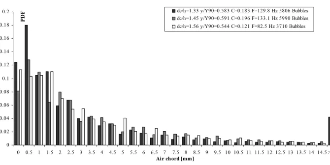
[Ø=0.25 mm ∆x= 7mm, ∆z=1.4 mm]. 0 0.02 0.04 0.06 0.08 0.1 0.12 0.14 0.16 0.18 0.2 0 0.5 1 1.5 2 2.5 3 3.5 4 4.5 5 5.5 6 6.5 7 7.5 8 8.5 9 9.5 10 10.5 11 11.5 12 12.5 13 13.5 14 14.5 >15 Air chord [mm] PD F dc/h=1.33 y/Y90=0.583 C=0.183 F=129.8 Hz 5806 Bubbles dc/h=1.45 y/Y90=0.591 C=0.196 F=133.1 Hz 5990 Bubbles dc/h=1.56 y/Y90=0.544 C=0.121 F=82.5 Hz 3710 Bubbles

Figure 4.2- Air chord size distributions (0 < C ≤ 0.3). Step edge No 10; Flow rate: dc/h=1.33

[Ø=0.25 mm ∆x= 7mm, ∆z=1.4 mm]; Flow rate: dc/h=1.57 Instrumentation: single tip probe

(3)

0 0.05 0.1 0.15 0.2 0.25 0.3 0 0.5 1 1.5 2 2.5 3 3.5 4 4.5 5 5.5 6 6.5 7 7.5 8 8.5 9 9.5 10 10.5 11 11.5 12 12.5 13 13.5 14 14.5 >15 Air chord [mm] PD F dc/h=1.0 y/Y90=0.707 C=0.528 F=163.3 Hz 7348 Bubbles dc/h=1.15 y/Y90=0.659 C=0.551 F=228.5 Hz 8000 Bubbles

Figure 4.3- Air chord size distributions (0.3 < C < 0.7). Step edge No 10; Flow rate: dc/h=1.0

Instrumentation: single tip probe [Ø=0.35 mm]; Flow rate: dc/h=1.15 Instrumentation: double tip

probe [Ø=0.25 mm ∆x= 7mm, ∆z=1.4 mm]. 0 0.05 0.1 0.15 0.2 0.25 0.3 0 0.5 1 1.5 2 2.5 3 3.5 4 4.5 5 5.5 6 6.5 7 7.5 8 8.5 9 9.5 10 10.5 11 11.5 12 12.5 13 13.5 14 14.5 >15 Air chord [mm] PDF dc/h=1.33 y/Y90=0.725 C=0.489 F=167.6 Hz 7688 Bubbles dc/h=1.45 y/Y90=0.732 C=0.521 F=168.9 Hz 7600 Bubbles dc/h=1.56 y/Y90=0.722 C=0.564 F=131.7 Hz 5927 Bubbles

Figure 4.4- Air chord size distributions (0.3 < C < 0.7). Step edge No 10; Flow rate: dc/h=1.33

[Ø=0.35 mm].

4.1.3 Normalised probability distribution functions of water droplet chords (C ≥ 0.7)

Present results included detailed air-water flow measurements for 0.7 ≤ C ≤ 0.999 and y/Y90 up to

2.5.Those date led to a better understanding of the complex nature of the spray. The analysis of the spray data suggested that the spray region may include three sub-regions with distinctive characteristics. That is for 0.7 ≤ C < 0.9, 0.9 ≤ C < 0.95 to 0.97 and 0.95 to 0.97 ≤ C ≤ 1.

(4)

For 0.7 ≤ C < 0.9 the probability distribution functions of the water droplet chords showed the same trend of the PDF of the intermediate region. That is the PDF followed a log-normal shape and the distribution functions were skewed with a preponderance of small bubbles relative the mean size. The maximum value of the PDF is about 0.13 and the largest water droplet chord size is between 0.5 and 3 mm. In Figures 4.5 and Figure 4.6 the probability distribution functions for several discharges at step edge ten are shown.

0 0.02 0.04 0.06 0.08 0.1 0.12 0 0.5 1 1.5 2 2.5 3 3.5 4 4.5 5 5.5 6 6.5 7 7.5 8 8.5 9 9.5 10 10.5 11 11.5 12 12.5 13 13.5 14 14.5 >15 W ate r chord [mm] PD F dc/h=1.0 y/Y90=0.965 C=0.883 F=60.6 Hz 2728 Droplets dc/h=1.15 y/Y90=0.926 C=0.855 F=100.2 Hz 4508 Droplets

Figure 4.5- Water chord size distributions (0.7 ≤ C < 0.9). Step edge No 10; Flow rate: dc/h=1.0

[Ø=0.25 mm ∆x= 7mm, ∆z=1.4 mm]. 0 0.02 0.04 0.06 0.08 0.1 0.12 0 0.5 1 1.5 2 2.5 3 3.5 4 4.5 5 5.5 6 6.5 7 7.5 8 8.5 9 9.5 10 10.5 11 11.5 12 12.5 13 13.5 14 14.5 >15 W ate r chord [mm] PD F dc/h=1.33 y/Y90=0.939 C=0.861 F=77.6 Hz 3448 Droplets dc/h=1.45 y/Y90=0.944 C=0.858 F=83.6 Hz 3763 Droplets dc/h=1.56 y/Y90=0.959 C=0.880 F=61 Hz 2743 Droplets

(5)

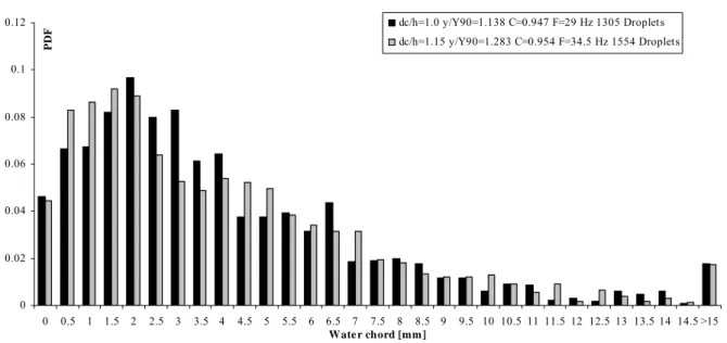
0 0.02 0.04 0.06 0.08 0.1 0.12 0 0.5 1 1.5 2 2.5 3 3.5 4 4.5 5 5.5 6 6.5 7 7.5 8 8.5 9 9.5 10 10.5 11 11.5 12 12.5 13 13.5 14 14.5 >15 W ate r chord [mm] PD F dc/h=1.0 y/Y90=1.138 C=0.947 F=29 Hz 1305 Droplets dc/h=1.15 y/Y90=1.283 C=0.954 F=34.5 Hz 1554 Droplets

[Ø=0.25 mm ∆x= 7mm, ∆z=1.4 mm]. 0 0.02 0.04 0.06 0.08 0.1 0.12 0 0.5 1 1.5 2 2.5 3 3.5 4 4.5 5 5.5 6 6.5 7 7.5 8 8.5 9 9.5 10 10.5 11 11.5 12 12.5 13 13.5 14 14.5 >15 W ate r chord [mm] PD F dc/h=1.33 y/Y90=1.152 C=0.952 F=33.3 Hz 1488 Droplets dc/h=1.45 y/Y90=1.155 C=0.951 F=36.5 Hz 1641 Droplets dc/h=1.56 y/Y90=1.136 C=0.950 F=30.1 Hz 1352 Droplets

[Ø=0.35 mm].

For 0.9 ≤ C < 0.95 to 0.97 the probability distribution functions of water droplets was flatter, a log-normal shape can not be clearly recognised. The largest probability of droplet sizes was between 0.5 and 2 mm where the probability distribution function reached about 0.11. The probability of large chord sizes was lower than that for 0.7 ≤ C <0.9.

(6)

For C ≥ 0.95 to 0.97 that is the upper flow region the flow structure consisted of individual ejected water droplets surrounded by air. The probability distribution functions did not follow a log-normal distribution. The PDF maximum value was about 0.15 and the largest probability of droplet chord sizes was between 1.5 and 2 mm.

0 0.02 0.04 0.06 0.08 0.1 0.12 0.14 0.16 0.18 0 0.5 1 1.5 2 2.5 3 3.5 4 4.5 5 5.5 6 6.5 7 7.5 8 8.5 9 9.5 10 10.5 11 11.5 12 12.5 13 13.5 14 14.5 >15 W ate r chord [mm] PD F dc/h=1.0 y/Y90=1.913 C=0.994 F=4.5 Hz 203 Droplets dc/h=1.15 y/Y90=1.907 C=0.992 F=6.6 Hz 295 Droplets

Figure 4.9- Water chord size distributions (C ≥ 0.97). Step edge No 10; Flow rate: dc/h=1.0

[Ø=0.25 mm ∆x= 7mm, ∆z=1.4 mm]. 0 0.02 0.04 0.06 0.08 0.1 0.12 0.14 0.16 0.18 0 0.5 1 1.5 2 2.5 3 3.5 4 4.5 5 5.5 6 6.5 7 7.5 8 8.5 9 9.5 10 10.5 11 11.5 12 12.5 13 13.5 14 14.5 >15 W ate r chord [mm] PD F dc/h=1.33 y/Y90=1.721 C=0.993 F=5.4 Hz 229 Droplets dc/h=1.45 y/Y90=1.647 C=0.992 F=6.9 Hz 309 Droplets dc/h=1.56 y/Y90=1.55 C=0.992 F=6.2 Hz 280 Droplets

Figure 4.10- Water chord size distributions (C ≥ 0.97). Step edge No 10; Flow rate: dc/h=1.33

(7)

4.2 Correlation analyses

Correlation analyses were performed for all data collected with two single-tip probes and with the double tip probes (Table 4.1). When two single tip probes were used, the reference probe was placed on the channel centreline (z=0) and the second probe was fixed at a known transverse distance z but at the same vertical and streamwise distances. When a double tip probe was used, the two probe sensors were located at the same vertical distance y, but they were separated by a streamwise distance ∆x measured with a microscope. In both cases, the two probe sensors were simultaneously sampled and their signals were analysed in terms of auto-correlation and cross-correlation functions Rxx and Rxy

respectively. Basic correlation analysis results included the maximum cross-correlation coefficient (Rxy)max, the characteristic time lag τ for which Rxx=0.5 (τ0.5)xx, the characteristic time lag τ for which

Rxy=0.5*(Rxy)max (τ0.5)xy, the time lag for which Rxy=0 (T0)xx, the time lag for which Rxy=0 (T0)xy. and

the integral time scales Txx Txy were: xx (R 0) xx xx 0 T R ( )d τ=τ = τ= =

∫

τ τ (4-1) xy xy xy max (R 0) xy xy (R (R ) ) T R ( )d τ=τ = τ=τ = =

_∫

τ τ (4-2) where

Rxx is the normalised auto-correlation function

τ is the time lag

Rxy is the normalised cross-correlation function between the two probe output signals.

(8)

Table 4.1 Summary of all discharges investigated with two probe sensors.

4.2.1 Auto and cross correlation analysis results

For each measurements point, the original data of 900,000 samples were segmented and sub-divided into fifteen segments of 60,000 samples. For each segment auto and cross correlation functions were calculated. All fifteen results were averaged to calculate auto and cross correlation functions for the respective measurement point. Figure 4.11 shows typical auto and cross correlation functions.

The correlation function showed similar patterns for all investigated flow conditions. The auto-correlation did not follow a Gaussian error function. For each measurement point and for all flow rates, the correlation function showed a distinctive peak and a Gaussian shape. The cross-correlation function was flatter than the auto-cross-correlation. In Figure 4.12 the distribution of (Rxy)max is

presented as a function of the void fraction at different step edge with the same transverse distance ∆z for the same discharge. The distribution of (Rxy)max exhibited a similar trend for all step edges. The

maximum value ranged from 0.3 and 0.4 depending upon the transverse probe separation ∆z when the void fraction was between 0.45 and 0.6. For all discharges, (Rxy)max had the highest values further

downstream of the inception point at the step edge ten. This result is related to the trend of Fmax at the

dc/h Instrumentation ∆x [mm] ∆z [mm] Step edge No 0 8.45 7 0 8.45 8 0 8.45 9 0 8.45 10 0 3.6 10 0 6.30 10 0 10.75 10 0 13.70 10 0 16.70 10 0 21.70 10 0 29.50 10 1.15 two single-tip probes [Ø=0.35 mm]

0 40.30 10 0 8.45 8 0 8.45 9 0 8.45 10 0 3.6 10 0 13.7 10 0 21.7 10 0 35.2 10 1.45 two single-tip probes [Ø=0.35 mm]

0 55.7 10 7.0 1.4 10 1.15 double-tip probe [Ø=0.25 mm] 9.6 1.4 10 7.0 1.4 7 7.0 1.4 8 7.0 1.4 9 1.33 double-tip probe [Ø=0.25 mm] 7.0 1.4 10 7.0 1.4 10 1.45 double-tip probe [Ø=0.25 mm] 9.6 1.4 10

(9)

macroscopic scale. As shown in Figure 3.8, the maximum value of the bubble count rate increases monotonically with x/dc, where x is the longitudinal distance and dc is the critical depth.

0 0.1 0.2 0.3 0.4 0.5 0.6 0.7 0.8 0.9 1 -0.01 -0.005 0 0.005 0.01 0.015 0.02 0.025 0.03 lag time [s] Rx x ,R x y Auto-correlation dc/h=1.15 Step 10 z=8.45 [mm] Cross-correlation dc/h=1.15 Step 10 z=8.45 [mm]

Figure 4.11-Typical auto and cross correlation functions. Flow rate: dc/h=1.15, Step edge 10

Instrumentation: two single-tip probes side by side [Ø=0.35 mm ∆z=8.45 mm]

0 0.05 0.1 0.15 0.2 0.25 0.3 0.35 0.4 0.45 0.5 0 0.1 0.2 0.3 0.4 0.5 C 0.6 0.7 0.8 0.9 1 (R xy)max Step 7 dc/h=1.15 Step 8 dc/h=1.15 Step 9 dc/h=1.15 Step 10 dc/h=1.15

Figure 4.12- (Rxy)max as a function of void fraction. Flow rate: dc/h=1.15, Step edges 7, 8, 9, 10

(10)

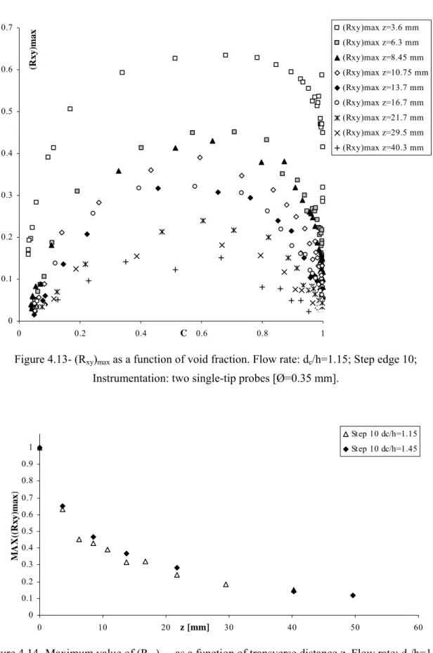
The cross-correlation function is strongly related to the transverse or streamwise separation distance between the two sensors. In Figure 4.13 (Rxy)max is presented as a function of the void fraction at step

edge ten for different transverse distance ∆z. (Rxy)max drops down as the distance ∆z increases. Figure

4.12 and Figure 4.13 show the results for dc/h=1.15 but the same patterns were observed for all

discharges. This is illustrated in Figure 4.14 where the trend of the maximum value of (Rxy)max is

presented as a function of the transverse distance ∆z at step edge ten for both discharges investigated. The maximum of (Rxy)max decreased with the increasing distance in a more than proportional manner.

For the greatest separation distances ∆z, the maximum of (Rxy)max was between 0.1 and 0.2 and it

seemed to drop to zero.

The distance between the two sensors also influenced the integral times: Txx and Txy. Txx represents the

integral time scale of the longitudinal bubbly flow structures (CHANSON 2006). It is the characteristic time of the eddies advecting the air-water flow interfaces in the streamwise direction. Txy

is a characteristic time scale of the vortices with a transverse length scale ∆z advecting the air-water flow structures. In Figure 4.15 Txx and Txy are presented in a dimensional form (unit: milliseconds) as

functions of the void fraction. They refer to dc/h=1.15 but similar trends were observed for all flow

rates investigated. The two integral time scales present the same patterns for void fraction C less than 0.95 even though the auto-correlation time scales Txx are larger than the transverse time scales Txy

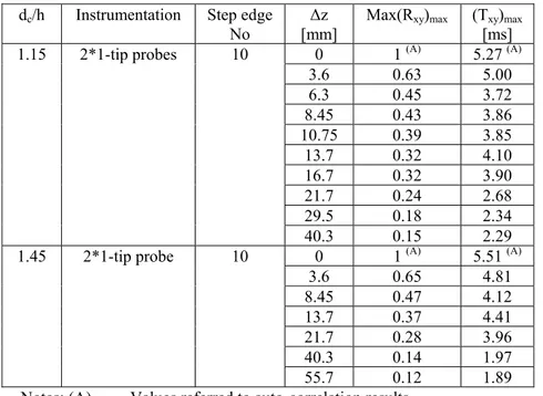
calculated for different distance ∆z as it is summarised in Table 4-2. Note in Table 4-2 and in Figure 4.16 that the integral time scale (Txy) was about independent of the transverse distance ∆z for 3 ≤ ∆z ≤

20 mm; for ∆z > 20 mm the larger is the distance between the two sensors and the smaller is the minimum value of Txy.

dc/h Instrumentation Step edge

No

∆z [mm]

Max(Rxy)max (Txy)max

[ms] 0 1 (A) _5.27(A) 3.6 0.63 5.00 6.3 0.45 3.72 8.45 0.43 3.86 10.75 0.39 3.85 13.7 0.32 4.10 16.7 0.32 3.90 21.7 0.24 2.68 29.5 0.18 2.34 1.15 2*1-tip probes 10 40.3 0.15 2.29 0 1 (A) _5.51(A) 3.6 0.65 4.81 8.45 0.47 4.12 13.7 0.37 4.41 21.7 0.28 3.96 40.3 0.14 1.97 1.45 2*1-tip probe 10 55.7 0.12 1.89 Notes: (A) Values referred to auto-correlation results

(11)

0 0.1 0.2 0.3 0.4 0.5 0.6 0.7 0 0.2 0.4 C 0.6 0.8 1 (R xy)ma x (Rxy)max z=3.6 mm (Rxy)max z=6.3 mm (Rxy)max z=8.45 mm (Rxy)max z=10.75 mm (Rxy)max z=13.7 mm (Rxy)max z=16.7 mm (Rxy)max z=21.7 mm (Rxy)max z=29.5 mm (Rxy)max z=40.3 mm

Figure 4.13- (Rxy)max as a function of void fraction. Flow rate: dc/h=1.15; Step edge 10;

Instrumentation: two single-tip probes [Ø=0.35 mm].

0 0.1 0.2 0.3 0.4 0.5 0.6 0.7 0.8 0.9 1 0 10 20 z [mm] 30 40 50 60 M A X ((R xy)max ) Step 10 dc/h=1.15 Step 10 dc/h=1.45

Figure 4.14- Maximum value of (Rxy)max as a function of transverse distance z. Flow rate: dc/h=1.15

and dc/h=1.45; Step edge 10; Instrumentation: two single-tip probes [Ø=0.35 mm].

(12)

The upper spray region consists primarily of ejected droplets which interact little with the surrounding air and the rest of the flow. The structure of the flow in the upper spray region is highlighted also in Figure 4.17 where Txx is presented as a function of the bubble count rate F for the same discharge at

different step edges. Txx shows similar trends but different order of magnitude. At step edge seven the

maximum value of the integral time scale is about 3.1 ms for F=165 Hz and at step ten the maximum value is ranging from 4 and 5 ms for F=200 Hz. This result is consistent with the macroscopic structure of the flow detailed in chapter 3. In paragraph 3.2.1 it was hinted that for all discharges, the bubble count rate as a function of the longitudinal distance from the inception point is increasing (Figure 3.5). 0 1 2 3 4 5 6 7 8 0 0.1 0.2 0.3 0.4 0.5 C 0.6 0.7 0.8 0.9 1 Txx Txy [ms ] T xx T xy z=3.6 mm T xy z=6.3 mm T xy z=8.45 mm T xy z=10.75 mm T xy z=13.7 mm T xy z=16.7 mm T xy z=21.7 mm T xy z=29.5 mm T xy z=40.3 mm

Figure 4.15- Txx and Txy [ms] as a function of void fraction. Flow rate: dc/h=1.15; Step edge 10;

(13)

0 1 2 3 4 5 6 0 5 10 15 20 25 30 35 40 45 z [mm] Tx y [ m s] C<0.3 0.3<C<0.7 0.7<C<0.9 0.9<C<0.95 C>0.95

Figure 4.16- Txy [ms] as a function of the distance z. Flow rate: dc/h=1.15; Step edge 10;

Instrumentation: two single-tip probes [Ø=0.35 mm].

0 0.5 1 1.5 2 2.5 3 0 1 2 3 Txx [ms]4 5 6 7 8 y/ Y 9 0 0 0.2 0.4C 0.6 0.8 1 T xx T xy z=3.6 mm T xy z=6.3 mm T xy z=8.45 mm T xy z=10.75 mm T xy z=13.7 mm T xy z=16.7 mm T xy z=21.7 mm T xy z=29.5 mm T xy z=40.3 mm Void fraction

Figure 4.17- Txx and Txy [ms] and void fraction as a function of y/Y90. Flow rate: dc/h=1.15;

(14)

0 1 2 3 4 5 6 7 8 0 50 100 F [Hz] 150 200 Txx [ms ] T xx Step 7 T xx Step 10

Figure 4.18- Txx as a function of the bubble count rate. Flow rate: dc/h=1.15; Step edge 7 and 10;