Configuration of programmable optical switches for filterless optical networks

(1)

POLITECNICO DI MILANO

Department of Electronics, Information and Bioengineering

Master of Science in Telecommunication Engineering

Configuration of Programmable Optical

Switches for Filterless Optical Networks

Supervisor:

Prof. Massimo Tornatore Co-Supervisor: Dr.Omran Ayoub Thesis Of: Faryal Fatima 864897 Academic Year 2018/2019

(2)

(3)

(4)

List of Figures

2.1 Architecture for Active Photonics vs Filterless Optical Network . . . 11 2.2 Filterless Optical Networking Concept [1] . . . 12 2.3 Detailed Architecture of Filterless and WDM node . . 13 2.4 Example: broadcast and select architecture of FONs . . 14 2.5 Filterless Fiber Tree Establishment . . . 15 2.6 An illustrative example: 6-Node network topology . . . 18

3.1 Architecture on Demand Node with modules [2] . . . . 29 3.2 Architecture on Demand Node with modules [2] . . . . 31

3.3 Programmable Architecture on Demand

Implementa-tion . . . 34 3.4 An illustrative example: 6 -Node Network . . . 35 3.5 Detailed node setup: Programmable filterless network

architecture . . . 36 3.6 Illustrative Example: 6 - Node programmable SDM

ar-chitecture [cite SDM paper 2] . . . 40 3.7 illustrative Example: a) Convventional ROADMS, b)

FON Vs c) Programmable optical white boxes in FON 42

3.8 Detailed node setup for a) Convventional ROADMS, b) FON Vs c) Programmable optical white boxes in FON [3] 43

(5)

3.9 Programmable vs Filterless . . . 45

4.1 Nodal Connection Representation . . . 49

4.2 Nodal Connection Representation With Paths . . . 50

4.3 Nodal Connection Conflict . . . 51

4.4 Illustrative Example: Node Connection Conflict for a 6-Node topology . . . 53

4.5 Illustrative Example: Node Connection Conflict for a 6-Node topology . . . 54

4.6 Example: Unidirectional Trees . . . 55

5.1 A Comparative Study . . . 59

5.2 Programmable-aware flow diagram . . . 60

5.3 Flow-Diagram for the heurtistic approach for FONs . . 69

5.4 Flow-Diagram for WDM . . . 73

5.5 An Illustrative Example: Programmable-unaware Ap-proach . . . 74

6.1 6-Node Network . . . 80

6.2 6-Node network: ILP vs Heuristic . . . 82

6.3 6-Node network: Average total spectrum utilisation . . 84

6.4 6-Node network: Average Maximum FSUs on a link . . 85

6.5 6-Node network: Average Number of Nodes Receiving Broadcast . . . 86

6.6 6-Node network: Average Hop Length . . . 87

6.7 6-Node network: Average Useful FSUs . . . 88

6.8 6-Node network: Average Unuseful FSUs . . . 89

6.9 6-Node network: 4 Set of uni-directional Trees for 30 Demands . . . 90

(6)

6.10 6-Node network: Programmable-Aware Nodal

Architec-ture . . . 91

6.11 Component Usage for 6-Node Network . . . 92

6.12 7-Node Network . . . 93

6.13 7-Node network: Average total spectrum utilisation . . 94

6.14 7-Node network: Average Maximum FSUs on a link . . 95

6.15 7-Node network: Average Number of Nodes Receiving Broadcast . . . 96

6.16 7-Node network: Average Hop Length . . . 97

6.17 7-Node network: Average Useful FSUs . . . 98

6.18 7-Node network: Average Unuseful FSUs . . . 99

6.19 7-Node network: 7 Set of uni-directional Trees for 42 Demands (node-pair) . . . 100

6.20 7-Node network: Programmable-Aware Nodal Architec-ture . . . 101

(7)

(8)

List of Tables

2.1 Coherent Transponders [4] . . . 20 2.2 Network Parameters For Filterless And Active Photonic(values

given in the bracket) Solutions[5] . . . 26 2.3 Main Features: Filterles vs Active Photonic . . . 27

(9)

(10)

Sommario

La costante crescita del traffico Internet e un aumento dei servizi af-famati di larghezza di banda hanno portato i fornitori di servizi a in-trodurre una vasta gamma di flessibilità nella progettazione della rete. Per far fronte a questa crescita a lungo termine è diventato essenzia-le che essenzia-le reti ottiche siano in grado di comprendere capacità elevata, efficienza dei costi e agilità. Tuttavia, le entrate per i fornitori di ser-vizi Internet rimangono indebitamente piatte, il che di conseguenza porta a uno squilibrio in cui le reti ottiche devono essere aggiornate mantenendo al minimo sia i costi di capitale che operativi.

Al fine di aggirare questo problema, è estremamente necessario inve-stire in soluzioni in cui CAPEX e OPEX possono essere minimizzati in modo equo. Una di queste soluzioni emergenti è stata textit reti ottiche senza filtro che mira a ridurre al minimo l’utilizzo di dispositivi attivi facendo uso di componenti passivi e l’agilità di rete è raggiun-ta da ricetrasmettitori coerenti nei nodi. Tutraggiun-tavia, questo incentivo si traduce in uno scambio di prestazioni -off dove a causa della loro architettura broadcast-cast-select abbiamo uno spreco di spettro. Al fine di far fronte allo spreco di spettro introdotto tramite FON, un’al-tra soluzione proposta che consente reti ottiche elastiche agili ad alta capacità è scatole bianche ottiche programmabili. Questi switch ottici

(13)

mirano a introdurre una flessibilit`a nell’architettura nodale, le mie por-te di input e output di mapping che utilizzano solo componenti passivi montati su un backplane ottico.

La flessibilità dell’architettura nodale mirerà a gestire l’incertezza del traffico e offrirà un’architettura di nodo flessibile in cui si possono for-mare sulla base delle esigenze delle nostre connessioni di rete. In questa tesi esamineremo come ridurre al minimo lo spreco di spettro totale in-trodotto attraverso reti senza filtro. Per affrontare questo problema, proponiamo una soluzione in questa tesi con l’obiettivo di ridurre lo spreco di spettro con un’implementazione di un algoritmo euristico che mira a ridurre tutti questi percorsi ripresi dalle mie richieste che por-tano alla copia dei segnali trasmessi a collegamenti non intenzionali . Per estensione con programmabilità nei nostri nodi, non solo ridurremo l’utilizzo dello spettro, ma ridurrà anche il numero totale di componen-ti usacomponen-ti. L’algoritmo proposto è stato testato per diverse topologie di rete con diverse metriche di misurazioni in cui possiamo concludere che la programmabilità nei FON mostra un vantaggioso compromesso tra l’utilizzo dei componenti e l’utilizzo dello spettro anche se confronta-to con le loro controparti tradizionali come multiplexer riconfigurabili add / drop.

(14)

Abstract

The unwavering growth of internet traffic and an increase in bandwidth-hungry services has led the service providers to introduce a broad range of flexibility in the network design. In order to meet this long-term growth it has become essential for optical networks to be able to encom-pass high capacity, cost efficiency and agility. However the revenues for the internet service providers remains unduly flat, which consequently leads to an imbalance where the optical networks have to be upgraded while keeping both the capital and operational costs to minimum.

In order to circumvent this issue there is a dire need to invest in solu-tions where capital and operational cost can be fairly minimised. One such emerging solution has been filterless optical networks that aims to minimise the usage of active devices by making use of passive com-ponents and the network agility is attained by coherent transceivers at the nodes.However, this incentive comes at a performance trade-off where due to their broadcast-cast-select architecture we have spec-trum wastage. In order to address the specspec-trum wastage introduced via FONs another proposed solution which enables high capacity and agile elastic optical networks is programmable optical white boxes. These optical switches aim to introduce a nodal architecture flexibility my mapping input and output ports utilising only passive components

(15)

mounted on an optical backplane.

The nodal architecture flexibility will aim to deal with uncertainty in traffic and offer a flexible node architecture where based on the needs of our network, connections can be formed. In this thesis we will in-vestigate how the total spectrum wastage introduced through filterless networks can be minimised. To address this issue, we propose a solu-tion in this thesis with the objective of reducing the spectrum wastage with an implementation of a heuristic algorithm that aims to reduce all such paths taken up my demands that lead to copy of the signals being transmitted to unintended links. By extension with programmability in our nodes not only we will reduce the spectrum utilisation but also reduce the total number of used components. The proposed algorithm has been tested for several network topologies with several metrics of measurements where we can conclude that programmablility in FONs show a beneficial trade-off between component usage and spectrum utilisation even when compared to their traditional counter-parts such reconfigurable add/drop multiplexers.

(16)

Chapter 1 Introduction

1.1 Overview and Motivation

The up-and-coming internet traffic has been nothing if not, consistent and evolving at a rate that has been a primary concern of internet service providers and network operators. The substantial increase in communication orientated internet services has opened floodgates of users that will only continue to grow even further in coming future. The projected forecast via Cisco shows that there will be an increase of 26%, it will be a triple of its value since 2017.

These services can range from video streaming in high-definition, cloud storage, file sharing and Internet of things are just one of the manifold services that will further contribute to an escalating traffic. Therefore much of an effort has been heavily invested in how to provision today’s network to meet all the demands. However, the question that arises at this point, will this provisioning also lead to an increase in cost? Which is most definitely yes. Bringing a user friendly experience such

(17)

as high data bit rates while utilising optical fibers that have been thus far substantially instrumental in sustaining this burden.

Consequently, the optical transport would have to be upgraded in or-der to meet the imbalance by augmenting transmission capacity and efficiency [6]. To further improve the performance and the efficiency of networks while keeping costs under control. One of the possible ways is to minimise expensive network equipment. Undoubtedly the recent advances in digital signal processing and utilisation of tunable trans-mitters and coherent receivers have contributed eminently to solutions that are potentially more cost effective.

Naturally, for long term traffic growth a solution that can encompasses cost efficiency without losing the operational advantages of an agile network will be our goal [7]. One of the proposed architectures is filterless optical networks (FONs) that eliminates the usage of active photonic devices that greatly reduces not only our operational cost but also capital cost by making use of passive devices such as splitters and combiners. The agility of our networks will be be observed with some obvious trade-offs that result as a consequence of utilising passive devices which leads to spectrum propagating past their destination nodes leading to spectrum wastage in FONs.

In the proposed scenario we are going to deal with a broadcast and select architecture where agility is concentrated to the network nodes that make use of tunable coherent transceivers. Where the desired wavelengths is selected from a pool of channels and new channels are added via passive splitters and combiner. Consequently, what we have is a solution that reduces the installed first cost (IFC), a lower failure rate and an ease of reconfigurability. Their inherent gridless

(18)

archi-tecture is naturally more suitable for elastic optical networking and the fiber tree establishment further ensure that multicast traffic is well supported by them.

The performance trade-off here is in terms of spectrum utilisation which is by far its major drawback. In order to implement FONs establishing fiber trees is one of the first steps that are deployed as is without any reconfigurability whatsoever. Although their integration in networks with smaller number of nodes as well as a good connec-tivity has shown promising results and added incentives of spectrum saving can be achieved while utilising flex-grid operations. However the broadcast select as well their non-reconfigurable fiber trees has led to exploring this field for more alternatives. Programmable optical switches have come out as a promising alternative to the hardwired trees and spectrum wastage in FONs. Programmable optical switches comprise of optical backplanes with reconfigurable switches that allow mapping input port to output ports. These programmable switches have introduced nodal architecture flexibility replacing the hardwired connections. However, programmable optical switches in FONs will only make use of passive devices and bypass any unnecessary compo-nent which results in saving on spectrum wastage that was introduced with FONs and also addressing the privacy issues that arises in FONs due to demands going past their destination nodes.

The configuration of our programmable optical switches will play a pivotal role in their application in FONs. The uncertainty of traf-fic demands entails that the network nodes ought to be substantially equipped to deal with the varying traffic demands. Several factors hugely contribute towards the immense need to have flexibility at nodes

(19)

in order to keep up with that level of uncertainty. However, over pro-visioning the network could potentially lead to way higher capital or operational costs. Therefore, our goal with programmable switches is to ensure meeting the varying traffic demands in our network while ensuring to save on spectrum. In FONs splitters at nodes with nodal degree greater than 2 leads to a split copy of each signal being carried to all the links with our approach we will aim to reduce all such links that lead to this spectrum wastage.

1.2 Thesis Outline

The goal of our thesis is to investigate an efficient placement and config-uration of programmable optical switches in filterless optical networks. In this thesis we develop a programmable-aware heuristic that aims to aims to form the nodal connection on optical backplanes in an at-tempt to reduce the increased total spectrum utilisation that results from broadcast and select architecture of filterless optical networks. In order to compare the performance of the programmable-aware heuris-tic we validate the numerical results by comparing them to an ILP presented in Ref.[3] and then we compare its performance to several other bechmark solutions such as a)filterless optical networks, b) Ac-tive photonic c) programmable-unaware (is a baseline benchmark that deals with programmability only for certain nodes in a network)

Therefore, to present a more comprehensive and a conclusive study the thesis has been divided into following chapters.

(20)

net-works, the design and establishment of fiber trees with illustrative examples. It also explains the resource allocation and presents a comparison between active photonic and FONs while shedding light on relevant related work.

• Chapter 3 Presents an in-depth analysis of programmability in FONs. The aim of the chapter is to present what flexibility in nodal architecture entails and how it aims to overcome the draw-backs introduced with FONs using illustrative examples. It also discusses related work to show a detailed comparison between active photonic, FONs and programmable FONs.

• Chapter 4 will go in further great detail explaining the problem statement devised. Moreover, in order to understand better the methodology that has been adopted in our work some concepts will have to be introduced that have been explained in great detail via illustrative examples and mathematical model.

• Chapter 5 Presents the heuristic approach for programmable-aware in order to perform a comparison between all our ap-proaches and methodologies followed to produce the necessary results for comparison.

• Chapter 6 discusses numerical results that have been produced utilising the previously mentioned heuristics in Chapter 5

• Chapter 7 summarises main takeaways drawn from the evalu-ations performed and discuss possible future extensions of the work.

(21)

Chapter 2 Filterless Optical Networks

This chapter focuses on the concept of filterless optical networks (FONs) while presenting a clear comparison to its traditional counter-part; ac-tive photonic based on reconfigureable add-drop multiplexers (ROADMs). The chapter also presents an in-depth analysis of the advantages and disadvantages of FONs.

2.1 Concept

Filterless optical networks pose as one of the recent popular solutions to meet future capacity requirements while keeping both capital cost and operational cost under control [5]. It replaces the traditionally used ROADMs based on wavelength selective switches (WSS) with passive devices such as splitters and combiners as shown in the Figure 2.1. Hence, the name ’filterless’ which preludes to its inherent architecture of replacing filters at network nodes with passive devices. The replace-ment of of active switching with passive couplers and splitters creates a

(22)

broadcast and select architecture in which the agility is utilised at the edge terminals by the coherent transceivers. Moreover, due to the re-cent development in transmission technology where advancements and breakthroughs in transmission impairment techniques, advancements in modulation formats and coherent transmitters and tunable trans-mitters substantially improved the reach WDM transmission systems [1]. Which by extension led to an easier integration of passive solutions such as filterless optical networks.

λ λ λ λ λ λ λ λ λ

Active Switching Architecture Filterless Architecture

W S S W S S Passive couplers

Figure 2.1: Architecture for Active Photonics vs Filterless Optical Net-work

FONs were first introduced in [7], the concept of FONs is based on utilising the agility of wavelength selective switching at the transmitter and wavelength discrimination at the receiver[5]. Figure 2.2 represents the FON based on passive devices interlinking nodes via splitters and combiners. The recent advances in transponders including modulation formats, electronics dispersion compensation and high-gain forward error (FEC) have significantly contributed towards the enhanced

(23)

im-plementation of wavelength division multiplexing (WDM). The FONs heavily depend on the coherent detection schemes and can be attained via the carrier frequency tuning without utilising active photonic de-vices at the given nodes. This improved performance can be taken advantage of with the help of placement of tuned local oscillator at the receiver, Which allows it to select the desired channel out of all channels received. The required channels are added to the band with the help of an optical combiner as shown in Figure 2.2.

Coherent Rx DSP- assisted tunable Tx Passive optical splitters/combiners 1 2 3 4 5 6 7 8

Figure 2.2: Filterless Optical Networking Concept [1]

The resulting architecture is only comprised of passive devices, which ultimately reduces our dependency on active photonic switching ele-ments. The work explained in Ref [5] explains further the methodology adopted in order to establish FONs. The interconnected fiber links are what we refer to as ’fiber trees’ which is an extension of light- tree

(24)

con-cept defined in Ref.[8]. In general a node with nodal degree d requires 2d 1:d splitters. Furthermore, these fiber trees are assigned to these lightpaths for unicast or multicast traffic.

Figure 2.3 shows a detailed nodal architecture of conventional WDM network compared to a filterless nodal architecture. A WDM node is comprised of a 2x1 WSS (active component) where the required wave-length is selected as per the nodes requirement. Whereas for a filterless node we observe a 2x2x2 broadcast and bridge (passive device).

Conventional node architecture Filterless node architecture

Figure 2.3: Detailed Architecture of Filterless and WDM node

FONs with their inherent passive architecture adhere to a broadcast and select architecture, therefore spectrum wastage is one of its major drawback. The unfiltered channels as shown in 2.4 represented by greyed out blocks, propagate all the way to terminal nodes in FONs. This leads to a significant increase in the spectrum consumption since

(25)

resources occupied by the unfiltered channels cannot be utilized by any other connection. Figure 2.4 shows the spectrum utilization caused by these unfiltered channels and how another connection cannot take up the same spectral resource. For instance we have a demand going from source node 1 to destination node 3, given our passive architecture links (2,4) and links (4,5) will also take up the the same unfilitered signal. Therefore, sources occupied by links (2,4) and (4,5) can not be reused by any other connection demand. Hence, exhausting the possibility of wavelength reusability on these links.

1 2 3

4 5

Demand between node 1 and 3 λ

Links (2,4) (4,5) receive the unfiltered signal (undesired FSU slots)

Links (1,2) (2,3) receive the desired FSU slots

(26)

2.2 Design of Filterless Optical Networks

As previously shown in Fig 2.4, FONs are based on broadcast and select architecture that leads to laser loops being formed, therefore establishing fiber trees is an imperative for their application and has become an integral part of its design. Before we apply routing and spectrum allocation algorithms, fiber tree establishment is of critical importance since it ensures the full connectivity between all the nodes in the network. Which by further extension determines the possibility of routing and spectrum allocation in our network. FONs are com-prised of passive devices which results in a local add-drop criterion that leads to broadcast in passive light trees. Since FONs inherently follow the drop-and-waste principle as shown in Fig. 2.4 therefore we have unfiltered signals going past their destination nodes and causing spectrum wastage. λλλλ λλ λλλλλλ λ λ λλ Fiber tree T1 Fiber tree T2 5 6 3 2 1 4

(27)

In Ref [5] and [7] we have been presented with a detailed filterless network design problem. Figure 2.5 represents a detailed illustration of the problems at hand. The goal is to establish fiber trees that not only ensure full network connectivity while satisfying all the demands but also ensure that all the nodes are physically connected [5]. The fiber trees establishment has to meet the following physical constraints in order to meet all the requirements that are addressed below:

• Laser loop constraint: The usage of passive devices such as splitters and combiners leads to the laser effect. The laser effect is a consequence of amplified spontaneous emission (ASE) due to the presence of erbium-doped fiber amplifiers (EDFAs) in optical links. Fig 2.5 describes how a loop is generated if we connect the nodes nodes 4 via a combiner and node 6 via splitter. (Figure 2.5 the red dotted line represents a laser loop ). As a consequence we will wavelengths circulating in our network if the connections are not physically terminated. So, the laser loops ensures that our utilised wavelengths will not circulate on our links.

• Fiber tree length constraint: While establishing our fiber trees any root-leaf combination must fulfill the criterion of not exceeding the maximum reach distance. The usage of passive devices further contributes to an insertion loss as well as the optical signal-to-noise ratio (OSNR) due to accumulated ASE which has to be accounted for in our link budget.

• Wavelength utilisation constraint: The broadcast and se-lect nature of FONs make them susceptible to wavelengths being forwarded past their destination node. The signal as well as

(28)

the ASE will be forwarded to the succeeding node. Therefore, its necessary that we choose filterless solution which reduces the number of wavelength used.

Figure 2.6 shows an illustrative example of fiber tree establishment and how demands are routed. In the given example we have a six-node topology and in totality five demands (D1 - D5). The list of demands are coloured coded in the box at the bottom right in Fig.2.3. The network is divided into 2 bidirectional fiber trees, Tree 1 (dashed line) and Tree 2 (straight line). The bidirectional lines following these trees represent the bi-directionality of our fiber trees. The demands D1, D2 and D3 are routed over tree 1 and assigned 3 frequency slot units (FSUs),2 FSUs and 3 FSUs respectively. Whereas D4 and D5 are routed and assigned 3 FSUs and 4 FSUs respectively over tree 2. The passive nature of FONs cause broadcast, in order to differentiate between the FSUs that are intended for a node will be referred to as the useful FSU whereas the broadcast FSU will be referred to as unuseful FSU that go past the intended nodes leading to spectrum wastage. The unuseful FSU in the figure is denoted with dashed small boxes with the respective colours of their demands (useful with a fuller box). The number of colour coded blocks represent the total number of FSUs taken up by each demand.

In the given example, demand D1 (blue) is routed over the tree 1 from source node 1 to destination node 6 taking up 3 FSUs. Given the topology of our tree 1 link (3, 5) will be the broadcast link for the demand 1. Hence why the link (3, 5) have a patterned blue blocks representing the unuseful FSUs. Following the demands, D2 (red) originates from source node 2 and terminates at node 6 hence taking

(29)

Unuseful FSU slot Useful FSU slot

5

1 6

2 3

4

Passive filterless network

D1: 1  6 (3 slots) D2: 2  6 (2 slots) D3: 3  5 (3 slots) D4: 6  2 (3 slots) D5: 5 4 (2 slots)

Figure 2.6: An illustrative example: 6-Node network topology

up once again link (3, 5) as the broadcast link (red patterned box). Whereas D3 goes from node 3 to node 5 with no broadcast since the link terminates at node 5. Demands D4 and D5 are routed on the tree 2 hence link (4, 1) receives the unuseful FSUs of both the demands. Whereas link (4, 2) only receives the unuseful FSUs of D5.

It can be witnessed via the example that some links suffer the broad-cast feature of the FON’s more than others. For instance, the link (4, 1) is purely taken up by unuseful FSUs whereas link (3, 5) takes the unuseuful FSU’s of D1 and D2 and the only useful FSU’s are of the demand D3. This spectrum wastage feature of FON’s is one of its biggest drawbacks. Moreover, it is necessary to mention at this point that FON’s offer a more static architecture which means that the fiber trees are not reconfigurable. Therefore, FONs have to rely on

(30)

other external features in order to accommodate the node configura-tion and link interconnecconfigura-tions. In order to fully utilize FON’s passive architecture while taking advantage of cost effectiveness another so-lution called, programmable filterless (PF) architecture was proposed. It helps alleviate the resulting spectrum wastage in FONs. PF archi-tecture will be dealt with in great detail in order to emphasize on its importance in FONs.

In Ref [5] the problem is divided into a two step problem. Where the first step is to establish the trees and the second step is to route all the given demands on the shortest path. Ref [5] further explains a fiber tree establishment algorithm, due to its obvious complexity with splitters and combiners a genetic algorithm (GA) was proposed to find near-optical solutions. GA helps in exploring possible solutions to our given problem by assigning arbitrary colours to our fiber links. Aspect such as, network’s connectivity and the average connection length are attributed to the fitness values of the given GA. The population with acceptable fitness are further chosen to expand our generation of new nearly optimal solutions.

2.3 Spectrum Wastage

Resource Allocation in FON’s is of crucial importance since their pas-sive nature offers a colourless grid, which by extension makes it easier for implementing elastic optical networking. Elastic optical networking ensures the spectral efficiency since channel spacing no longer adheres to the restrictions imposed by International Telecommunication Union (ITU). Several demands based on their capacity and distance will be

(31)

as-signed bandwidths. FON’s with their passive architecture make them inherently suitable for elastic optical networking since FONs do not require replacement of devices at nodes (filters etc. as opposed to its traditional counterpart active photonic that requires replacement of switching devices. Hence, gridless operation can be achieved with no cost for FONs since in active photonics it requires the deployment of wavelength selective switches for gridless architecture which costs significantly more than FONs.

Table 2.1: Coherent Transponders [4]

Line rate Modulation Format Channel Bandwidth Reach(km)

100 DP-QPSK 37.5 2000

200 DP-16QAM 37.5 700

400 DP-16QAM 75 500

The second step after exploring the possible optimal solutions for our fiber tree establishment is spectrum allocation. The [9] deals with a tabu search metaheuristic that has been adopted for the work in Ref [5] for wavelength assignment. To uphold the wavelength singularity constraint if there exists a common link in the given demands, it forces it to choose an assignment of different colour. The work in Ref [4] takes a different take on resource allocation by proposing a heuristic algo-rithm for static routing and spectrum allocation(RSA). All the nodes in a given physical topology are equipped with coherent transponders in the table 2.1. The proposed methodology compares the fixed-grid to elastic filterless. The heuristic takes the network topology and traffic matrix as the input, while carrying out routing and then the spectrum allocation. A multi period traffic is considered while choosing shortest

(32)

path in the fiber trees while choosing the most spectrally efficient line rate that meets the connection demands path length. It also considers several ordering policies for example the longest distance first (LDF) the hights line rate first (HLF) and most demanding first (MDF). The algorithm first checks if the demand can utilise the existing used FSUs for the same source and destination node otherwise it will allocate the first available spectrum. Spectrum utilisation is one of the main measuring features for the algorithm. It makes use to several toppolo-gies in order to analyse the performance elastic versus fixed-grid. The result shows that for high traffic loads RSA-EF shows a remarkable im-provement spectrum utlisation compared to fixed-grid cases. however, for low traffic levels this difference is not marginal in fact it almost non-existent.

The work in Ref [6] also deals with routing and spectrum assignment in elastic FON’s. It proposes an integer linear program in order to find optimum solutions for smaller topologies. Wheras for bigger topologies two heuristics are proposed in order to alleviate spectrum utilisation. For ILP only single traffic period is considered due to to computational complexity whereas the two other proposed heuristics will deal with a long-term growth of the given traffic. Like before, the first step in implementing RSA is to select the spectral and cost efficient line rate while choosing the shortest path for our connection demand in fiber trees. It assigns the number of FSUs to each demand while ensuring that the maximum number of FSUs remain within its minimum limit. Due to complexity reasons the RSA problems here has been divided into routing and spectrum allocation in order to be dealt with sequen-tially. The results remain consistent with previous work that indeed for

(33)

bigger topologies flex-grid does indeed offer grater saving on spectrum utilisation.

At this point we have seen despite FONs with all its highlighting fea-tures result in spectrum wastage which is by far its major drawback and needs to be addressed if its application has to be considered more widespread. One of alternatives while saving on cost was to introduce a hyrbid solution. This solution is refereed to as semi-filterless since only certain nodes will be filtered.

2.4 Semi-Filterless

FONs have already established what they offer with their passive ar-chitectures but spectrum wastage remains as is one of its major draw-backs. Several methodologies have been explained in order to imple-ment FONs in order to improve its performance for it be able to be considered as a viable solution. One of the possible proposed ideas has been Semi-Filterless which as the name suggests is a hybrid solution. On top of FON’s you place filters at strategic location in a given net-work hence the name semi-filterless. FONs architecture have already proven that their broadcast feature leading the demands going past their destination node hence, utilising more wavelengths for the same demands than its counter-parts such as active photonic solutions.

Semi-filterless solution propose to use passive coloured components as mentioned from work in Ref [10]. It makes use of fiber Bragg-grating (FBG) at certatin nodes in order to reduce wavelength usage and en-sure that FON’s can be taken full advantage of in terms of its cost

(34)

effectiveness. The placement of filters has to be decided strategically in order to ensure that the incoming wavelengths that are redudant can be dropped. The work in Ref[10] deals with a proposed solution for the placement of these filters in the network. Given several fiber trees it picks the one that requires maximum number of wavelengths, and then chooses to place a filter where at a node that effects a large number of edges hence, decreasing the number of utulised wavelengths.

The gathered results are considered for several network topologies as well as a uniform and non-uniform traffic. The simulation results allow us to conclucde the obvious that the more the number of filters used the less is the wavelength usage. however, its necessary to mention that despite the placement of these filters there reaches a point where any futher addition to these filters leads to a saturation, implying that the number of wavelengths are not directly propotional to the usage of filters in our network. Hence, there is a limit to which we can add filters to out FON’s thereby achieving the results we want any further addition does not help us improve the performance of FONs. However, with a minor increase of cost we can achieve remarkable results with utilising filters are certain nodes.

2.5 Related Work:

Filterless vs Active

Photonic

This section summarizes the main advantages and disadvantages of filterless optical networks and discusses related work and highlights the main differences bet wen filterless and active photonic networks.

(35)

Some of the main advantages of FONs are as following:

• cost-effectiveness: Since the network is provisioned with passive devices such couplers and splitters the overall cost of network is remarkably reduced which ultimately reduces both capital and operational cost making it a preferable choice.

• Robustness and energy efficiency: The utilisation of passive de-vices allows it be less prone to failures and hence less effort are required for its upkeep which also reduces overall the power con-sumption with FONs.

• Agility: Since we configure only the terminal nodes in FONs compared to ROADMS therefore the network is much faster due to its simplicity.

• Flex-grid colourless ability: FONs passive architecture inherently make them favourable for elastic optical networking.

• Mutlicast capability: Fiber trees establishment in FONs favourably accommodates mulitcast traffic in networks.

However, with all its above mentioned advantages, FONs suffer im-mensely due to their passive nature such as:

• broadcast and select: It leads to an architecture where the re-quested demands go past their destined nodes. In fiber trees each demand due to splitters is forwarded to all branches which adds to an increased spectrum consumption and also respective links utilised can not be further used by any other demand.

(36)

• no reconfigurability: It is comprised of inherent fixed fiber tree architecture which is established once and remains the same in order to meet all the requirements without any reconfigurability

• privacy issue: Demands travelling past their destination nodes that are raise privacy issues in FONs.

In order to describe more some of the existing work in the literature and present a comparative analysis between active photonic and filterless. The following metrics are considered in Ref[9][5] in order to draw the necessary conclusions:

• Network cost

• Wavelength utilisation

• Average demand length

• Average number of fiber link segments per demand

Several network topologies have been considered in [5] in order to val-idate the results for FON’s in the light of several optimization param-eters. The work in [7] and [1] considers: 7-node German network, 17 - node Italian network and the 17-node German network. (insert fig-ures of 7- node and 10- node network). The work assumes to have a uniform traffic between all the nodes. Therefore, a wavelength for every connection one of the only physical impairment assumed in these simulations is of system’s reach constraint (1500 km). The proposed solutions meet all the constrains as mentioned in section 2.1.1 above. Due to the broadcast nature of FON’s each demand can be routed on

(37)

more than one path. which leads to a protection for some of the de-mands. Although not fully discussed but it can be assumed that extra traffic protection is possible by utilising complementary fiber trees.

In order to compare the performance of our FON’s in with the ROADM’s that utilize WSS at each node. In order to fully utilize it’s capacity the work in [9] assumes to have a total of D WSSs were required with a node degree D greater than 2. The table below summarizes some of the numerical values for the 3 above mentioned topologies. For the purpose comparison routing was carried out on the shortest path for each demand. Although it’s brought up in Ref. [5] and [9] that the process has not been completely fair for active photonic since a lower wavelength utilisation can be achieved via optimizing that fiber link connection. However, regardless of the lower values of active photonic it can be clearly seen that FONs prove to be a promising solution since the values compare well for wavelength utilization. Furthermore we can conclude that given for comparable wavelength utilization FONs offer a significant reduction on cost.

Table 2.2: Network Parameters For Filterless And Active

Pho-tonic(values given in the bracket) Solutions[5]

Network 7-Node 10-Node 17-Node

Average Demand Length 374(349) 488(407) 480(414)

Average no.of fiber link segments 1.57(1.51) 2.27(2.02) 3.16(2.84)

No.of wavelengths 37(30) 28(28) 88(82)

Added Cost(a.u) 0.32(91.8) 0.36(122.4) 1.04(193.8)

(38)

technolo-gies. However we can not underestimate the fact that these trade-offs are substantially based on their applications. Since filterless solution has proven to be a valuable substitute to active photonic in smaller networks where network traffic is relatively lower and the trade-off between spectrum utilisation and cost can be favourably capitalised. For similar reasons, as the size of our network grows bigger we can witness FONs performance reducing largely due to a higher spectrum utilisation compared to active photonic. Therefore, FONs advantages and drawbacks are purely application be based and be improved due to several enabling technologies that will discussed further in coming chapters.

Table 2.3: Main Features: Filterles vs Active Photonic

Charatertistic Active Photonic Filterless

Cost higher lower

Spectrum Utilisation lower higher

Agility lower higher

Reliability(failures) higher lower

Demand path length lower higher

To address the drawbacks introduced by FONs especially that of spec-trum wastage one of the proposed solutions has been, nodal architec-ture flexibility. The said flexibility is offered via programmable optical switches while making use of passive devices. Their aim is to rectify the issues that were brought up by FONs and allow a flexible integration of FONs. The upcoming chapter will introduce these programmable switches and go in detail regarding their implementation and usage.

(39)

Chapter 3 Programmable Optical

Filterless Networks

In this chapter we first present the concept of architecture on demand (AoD) and its concept while also discussing the advantages it presents. We then go on to discuss the programmable optical switches while presenting their application in FONs and how the its implementation helps alleviate some of the drawbacks raised with FONs.

3.1 Concept: Architecture On Demand

The uncertainty of traffic demands entails that the network nodes ought to be substantially equipped to deal with varying traffic. Several factors hugely contribute towards the immense need to have flexibility at nodes in order to keep up with that level of uncertainty. One way to deal with this uncertainty is provisioning our network with more equipment, but that could potentially lead to way higher capital or

(40)

operational costs and inefficiency. Alternatively, we can provision the network with equipment that specifically deals with uncertainty that has to be addressed.

Figure 3.1: Architecture on Demand Node with modules [2]

Architecture-on-demand (AoD) or node architecture flexibility as the name implies allows us to have a great deal more control over the de-sign of our network nodes. As show in in figure 3.1 we can observe the architecture modules mounted on the optical backplane mapping the input ports to output ports. It is already established that AoD compared to the traditional static nodes will provide a greater deal of freedom to design the node’s architecture as per our requirements. Thus far, we have observed that several studies have investigated how to meet the requirements of varying traffic but the constraint imposed due to hardware limitation has been of little or no focus.Ref [2]

(41)

cap-tures the essence behind the node architecture flexibility and how we can capitalise on this technology. Moreover, its explains the enabling technologies for AoD and how elastic optical network plays a vital role in implementing a combined flexible network that meets the ever varying network requirements.

Various networks will pose varying constraints that need to be met, for instance routing different demands to various different destinations or dealing with traffic demands with mixed bitrates. Several propositions and in particular elastical optical networking has been of great interest in order to deal with these high stake demands. Despite it being a popular solution to the flexible allocation of spectrum it still fails to address some aspects of our requirements. One of the notable of them being of mixed bandwidth requirements that get defragmented and fail to accommodate higher bandwidth due to the lack of consecutive frequency slots [11]. Therefore, an approach that captures the diversity of traffic and deal with several functionalities such as switching, elastic allocation etc.

As represented in Figure 3.1 we can analyze an AoD architecture that is comprised of an optical backplane. An optical backplane is basi-cally a collection of electrical connectors that ensure all the optical connection on a circuit board are connected to each other. It is used to connect multiple devices passive or active mounted on top of this backplane supported by a printed circuit board (PCB) depending on our requirement for the node. An Optical backplane such as shown in the Figure 3.1 can be comprised of microelectromechanical systems (MEMS) that is connected various devices mounted on our backplane ranging from input output ports to spectrum selective switches (SSS),

(42)

Figure 3.2: Architecture on Demand Node with modules [2]

EDFA, spectrum defragmenter etc. All these connections can be con-nected via the optical backplane in a personalized fashion where the connections are not static or hard-wired as the standard nodes. This feature of AoDs allow them to make use of programmability on an extent where without any physical intervention these connections can be modified as per our requirement. This level of customization allows AoD nodes to have a higher precedence over the static nodes where such connections are hard wired and there is less room for making any such changes in our nodal architecture.

On one hand, the connections between modules themselves and be-tween programmable switches and modules are software-controlled, which adds to its flexibility. But on the other hand, it has to be mentioned that the number of modules and optical switches used are purely dependant on a nodes functionality and the demands it caters. Therefore, the nodal architecture flexibility purely depends on its usage in the network. Furthermore we can establish that despite introducing

(43)

the programmability in FONs in order to improve its performance. We are also making sure that based on networks requirements only use the modules that we need for a certain node, not only will this aspect help reduce its cost but also insertion losses are reduced. Programmability in FONs means our optical backplane or optical white box will only be comprised of a single optical switch per node utilising only passive devices.

Flexibility in nodes encompasses numerous factors from supporting varying bitrates to modulation formats but to narrow-down our crite-rion of comparison we want to focus more on architecture flexibility and routing. The work in Ref [11] has taken it further to explain further what each flexibility in AoDs entails:

• Switching Flexibility: Since the configuration can be varied over time it allows the system to map input to outputs ports in various ways. We have also observed that several optical devices offer flexibility for instance SSS slices its spectrum in several sizes and transmits them on different channels. Therefore with several such devices switching flexibility can be enhanced even more.

• Routing Flexibility: Its the systems capability to route a de-mand on more than one potential paths. This type of resilience in network is necessary in case of failures where back-up paths could be needed in order to reduce downtime. It allows to flexibly reroute the demands on alternative paths.

• Architectural Flexibility: One of the highlighting features of AoD is its ability to restructure the mounted modules. The rearranging of modules and input output ports allows to deal

(44)

with ever varying traffic demands.

3.2 Programmablility in Filterless

Opti-cal Networks

3.2.1 Configuration of a Programmable Optical

Switch

So far we have established that the flexibility in nodal architecture has been instrumental in dynamic reconfigurability of optical interconnec-tions; not only this addresses our concerns of limitations in hardware but the added benefits of saving on spectrum is what we will go in detail in coming discussion. As discussed in previous chapter, we have already made a point that FONs with all its advantages brings forth the issues of spectrum wastage. Which by extension also leads to pri-vacy issues since drop-and-waste feature of our passive nodes (splitters and combiners) will mean that our demands are going past their desti-nations nodes. Optical fiber trees establishment in FONs also raise one of the concerns regarding the hard-wired nature of FONs with little to no room for reconfigurablilty. Mainly to address all these drawbacks of FONs one of the novel solution of programmable optical networks based on filterless using optical white boxes [3]. The goal is to min-imize the spectrum utilization with programmablility in FONs while taking advantage of its passive nature.

As shown in Figure 3.2, an optical backplane is comprised of active devices such as MUX/DEMUX, SSS. Now we will deal with the

(45)

pro-Figure 3.3: Programmable Architecture on Demand Implementation

grammability implemented in FONs which implies making use of only passive devices such as splitters and combiners mounted on our optical backplane. AoDs with optical switching allow it to assign input to out-put ports bypassing unnecessary components. Not only this reduces spectrum wastage, but also reduce our cost and power consumption that are just one of the few upsides of utilizing nodal architecture felx-bility via optical white boxes. The goal is to find opitimized ways of routing our demands between nodes in order to reduce the used com-ponents as much as possible which in trn decreases further spectrum wastage compared to our previously proposed FONs solution.

To further support our claims we will use an illustrative example as shown in Figure 3.3 supporting programmable optical switches in FONs. We have a set of 5 unidirectional demands considered in a 6

(46)

5

1 6

2 3

4

Programmable filterless network

Figure 3.4: An illustrative example: 6 -Node Network

-node network for simplicity reasons. Each coloured coded demand is represented by a fuller coloured block in order to signify that its a useful set of FSUs (as shown in the block at bottom left) and shaded block to signify it is an unuseful FSU i.e broadcast FSUs where the demand goes to unintended links past their destination nodes. The example is an extension of FON in previous chapter therefore the goal is to show that with nodal architecture flexibility can help performance in FONs. Demand 1 going from node 1 to node 6 and demand from node 2 to node 6 will both no more go on link (3,5) since nodes 1,2 do not directly communicate with node 5 hence this connection can be considered ’cut’. Which means that node 2 can be directly con-nected to node 6 that will also include the demand coming from node 1 without splitting at node 3 (that we have witnessed happening with

(47)

FONs).

Meanwhile the demand from node 3 towards node 5 will just be an add signal without being forwarded to node 6 and reducing spectrum wastage considerably. The same scenario is assumed for the demand originating from node 6 towards node 2 (yellow blocks) where this demand will be no longer forwarded on links (4,1) hence avoiding the spectrum wastage that had results due to fiber trees in FONs based solutions. This flexibility not only reduces spectrum wastage but we are also bypassing unnecessary components, that helps save on power utilisation as increase the cost effectiveness of our overall network.

4 1 2 5 1 2 5 Drop 5 1 6 2 3 4

Unuseful FSU slot Useful FSU slot Passive Splitter/Coupler 2 6 5 2 6 5 Add 3

Figure 3.5: Detailed node setup: Programmable filterless network ar-chitecture

(48)

3.2.2 Application of Programmable Optical Switches

in FONs

Figure 3.5 is an extension of Figure 3.4, where we can also observe the nodal architectures for node 3 and node 4. The small black shaded blocks represent passive devices such as splitters and combiners. We can clearly see that issue of spectrum wastage due to splitters at our nodes has been addressed for node 3 and the demands intended for a node are transmitted to the said node. The general rule of thumb is that a node with node degree 2 will need 2d SSS in addition to a splitter and a coupler. In programmable each node is provisioned with an NxN optical switch and the size of it relies on our nodal degree.

Despite the upside of utilizing nodal flexibility will not inherently result in addressing all our concerns regarding the passive nature of our pro-posed solutions. This issue is pictorially explained further via Figure 3.4 we can observe the demand originating from node 5 going towards node 2 (yellow) and the demand from node 5 intended for 4 must past through a splitter and use the link (2,4) hence, not entirely avoiding the spectrum wastage. The nodal architecture of node 4 shows that it has to pass through splitter and the node 2 receives the split copy of demand 5 on link (4,2) (represented with a dotted line).

This goes to show that although nodal architecture flexibility has proven to be of great advantage but the dilemma remains as to how well can we encompass all the advantages nodal architecture flexibility has to offer. Analysing the example in Fig. 3.5 we can comprehend that introducing nodal architecture flexibility alone, will not be sufficient to address all our concerns that were brought up by FONs. Therefore, it

(49)

can be concluded that a programmable-aware approach for deploying programmable optical switches can be benefited from. The methodol-ogy will aim to structure the network in a way where the split copies of signals going to unintended nodes will be reduced and routed on another path in a programmable-aware fashion.

We clearly see through the above given illustrated examples that all our concerns that were raised with pure filterless have not been en-tirely addressed. We have discussed thus far in great depth how nodal architecture flexibility in FONs could help alleviate a part of our con-cerns. But in order to fully take advantage of programmable we must address concerns that were raised in the Fig. 3.5 (nodal architecture of node 4). The placement of splitters makes it unavoidable for some demands to avoid being split and contribute to spectrum wastage. One of the main goals here has been to capitalize fully on programmabil-ity in nodes specifically in FONs. We want to establish further on a methodology that can be adopted so the splitting of signals near these nodes can be potentially avoided. One of the proposed ideas that has been heavily investigated in this thesis has been to alleviate this issue and reduce spectrum wastage as much as possible.

3.3 Related Work on Programmable

Nodal architecture flexibility compared to FONs has been pretty recent and only limited amount of research has been done. The work in Ref [3] introduced optical white boxes application in FONs, by proposing their potential as a plausible solution to the obvious downsides of pure FONs. The work proposed a routing modulation spectrum allocation

(50)

solution as integer linear program (ILP) with objective of minimizing the maximum FSUs. The work has been compared to traditional active photonic vs filterless optical networks vs programmable optical white boxes in FONs. A 6-node network was utilized for the ILP solution and the results were compared to ROADM and FONs. Furthermore a 7-node network was also used but due to scalability issues for FONs a heuristic was used and the results were compared as before. The performance of optical white boxes is clearly proves our hypothesis to stands correct that the flexibility in nodal architecture shows re-markable improvement in results compared to FONs where spectrum wastage on average is about 15-20 % and the values are almost compa-rable with ROADMs for smaller network. As an output we also observe the required switch size, number of used couplers, maximum coupler degree. Clearly there is trade off between used components between optical white boxes in FONs and a passive filterless network.

The already established ground for nodal architecture flexibility fur-ther paved the path for investigating FONs combined with spatial di-vision multiplexing (SDM). SDM had been proposed in order to fill the gaps that programmability in FONs like spectrum wastage could not be compensated for while maintaining a pure filterless network. The elimination of copies of signals due to passive devices can be carried out by using a single-core fiber (SCF) where copy of each signal will be spatially separated into different fiber cores. This way the signals reach their destination without any splitting and causing unfiltered signals to reach past their destination.The work in Ref [12] formulated routing, modulation format, spectrum, core allocation (RMSCA) for programmable filterless networks as an ILP while reducing the cores

(51)

utilized and spectrum resource usage. A 7-node network topology was used and compared to wo benchmark solutions; passive filterless, PF-SCF architecture. Results show that PF-SDM reduces spectrum re-sources to almost 29 (add sign) compared to FONs. Although this implies that they PF-SDM solution utilizes on average will require more spectrum resources. In general programmable solutions will al-ways utilise less passive devices with lower max degree compared to FONs.

Figure 3.6: Illustrative Example: 6 - Node programmable SDM archi-tecture [cite SDM paper 2]

The work in [13] investigates further space division multiplexing in pro-grammable filterless networks, by proposing a binary particle swamp optimization (BPSO) to address the routing modulation format, spec-trum and core allocation (RMSCA) as before by reducing the

(52)

maxi-mum backplane size and reducing the used passive devices. Figure 3.5 shows an illustrative example for a 6-node network with programmable optical backplanes incorporated with SDM in order to lower spectrum wastage.The work proposes a two-objective BPSO-based hardware-aware RMSCA. The proposed solution has been divided into 2 parts; a heuristic candidate route evaluation algorithm (CREA) and another algorithm is utilised in order to carry out spectrum assignment. The performance in this work has made use of more realistic networks such German network topology with 11 nodes and 68 unidirectional links and a NSF network with 14 nodes and 42 unidirectional links, non uniform traffic scenarios are used. Tests were run by adding new de-mands The results are compared to 2 benchmark solutions such as shortest path (SP) and random selection of path (RP). For different traffic loads results show that NSF network utilizes less number of couplers. For increasing traffic demands clearly a higher number of couplers are required in order to meet the demands. However for lower traffic instances a lower backplane size is required.

3.4 Summary: Programmable Vs

Filter-less

To give our discussion a more conclusive shape we will at this point compare our proposed solutions with our our traditional WDM net-works as well. With FONs we have seen in previous chapter that the usage of passive devices (couplers and splitters) and the routing of de-mands via fiber trees which are inherently fixed once established. The passive nature of out network results in a ”drop and continue”

(53)

archi-tecture which preludes to demands travelling past their intended nodes and thus causing broadcast. Which throughout this discussion and il-lustrative examples has been referred to as the unuseful FSUs that are the unfiltered signals due to splitters at nodes instead of filters. Which eventually results in copies of signals going to each branch and result-ing in spectrum wastage. which raises many concerns such as privacy issues, spectrum wastage etc. The illustrative example in Figure 3.5 shows it for the 6-node network (already explained in chapter 1 in great detail).

5

1 6

2 3

4

Passive filterless network

5

1 6

2 3

4

Programmable filterless network

5

1 6

2 3

4

Conventional ROADMS

Figure 3.7: illustrative Example: a) Convventional ROADMS, b) FON Vs c) Programmable optical white boxes in FON

The already established ground for FONs allowed to introduce pro-grammability in these networks and establish a new paradigm where we could take advantage of FONs. Programmability or nodal

(54)

architec-a) b) c)

Figure 3.8: Detailed node setup for a) Convventional ROADMS, b) FON Vs c) Programmable optical white boxes in FON [3]

ture flexibility in filterless networks replaces the traditional hard-wired node connection with optical white boxes that are optical backplanes via which node connections can be formed as per our requirement. They support the usual network traffic by mapping input and output ports. Our goal is to dimension these nodes through programmable optical switches in such an optimized way where we utilize less devices (splitters or couplers) and also save a part of spectrum wastage that results due to FONs and is unavoidable. The reduced usage of compo-nents while forming our connection in programmable optical switches would not only result in less power consumption but also a reduced cost.

(55)

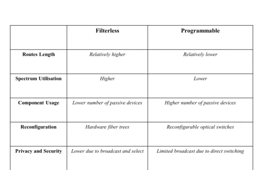
be-tween FONs application and Programmable optical white boxes while also observing our WDM networks. We see that the the spectrum wastage at Node 3 clearly has been addressed through connecting node 2 to node 6 directly via fiber switching where we avoid passing through a splitter as we can see in FON solution. which results in split copy of a signal being forwarded to link (3,5) and link (3,6). For demand 3 (brown) we can see that for programmable it can be replaced with a direct Add on node 3 towards node 5 without any split copies of other demands. However we can observe that for demand 4 and demand 5 since they are not meant for the same output have to be split before reaching their respective destination nodes. Whereas for WDM net-work each demand reaches the intended node without any hassle util-ising the shortest path. Furthermore, we can observe in Fig.3.8 that node setup for programmable node shows that it utilise less passive devices (couplers and splitters) compared to FONs. programmability also introduces that added incentive of fiber switching resulting in a lower insertion loss by utilising less ports of optical backplane.

Figure 3.7 shows a detailed nodal architecture of a) conventional ROADMs, b)Filterless optical networks and c) Programmable optical white boxes. The figure helps illustrate the main architectural differences between our proposed solutions. Each network is dimensioned such that so it can cater to all the network traffic demands. Furthermore, as men-tioned before, node 3 is represented from a 6-node network topology where in ROADMs in totality a 2d spectrum selective switches and a splitter or a combiner near to add/drop side. Whereas in filterless scenario a node with nodal degree d will utilise 2d 1:d splitters and combiners hence, in our configuration. Lastly, we have the

(56)

configura-tion of our programmable switches that where each node makes use of NxN that purely depends on our nodal degree.

Filterless Programmable

Routes Length Relatively higher Relatively lower

Spectrum Utilisation Higher Lower

Component Usage Lower number of passive devices Higher number of passive devices

Reconfiguration Hardware fiber trees Reconfigurable optical switches

Privacy and Security Lower due to broadcast and select Limited broadcast due to direct switching

(57)

Chapter 4 Configuration of

Programmable Optical

Switches in FONs

This chapter presents the problem of our thesis and explain in detail the methodology and concepts that have been adopted in order to formulate a model for a hardware-aware placement and configuration of programmable optical switches in FONs.

4.1 Problem Statement

The problem of programmable-aware placement and configuration of optical programmable switches is stated as follows:

• Given:

(58)

represents network nodes, and E is a set of arcs that repre-sent the network’s fiber links (edges).

– A uniform traffic matrix is considered where a node-pair set of demands is considered in order to provision the whole network

• Decide: The placement and configuration (optical node switch connections) of programmable optical nodes while performing spectrum allocation in a programmable-aware fashion.

• Objective: Minimise the total overall spectrum consumption in terms of FSUs

• Constraints:

– Satisfying all demands in the network

– Avoiding laser loops due to the utilisation of splitters and combiners

4.2 Nodal Connections

4.2.1 Nodal Connection Formation

In order to establish a background of what will be discussed in the coming chapters regarding the problem statement there are certain as-pects of the methodology that has to be formally introduced in order to establish a ground where our proposed solution to spectrum wastage in FONs has been addressed with a smart placement of programmable.

(59)

One of them being tuples or more formally termed as node connec-tion in this thesis basically refer to a list of 3 nodes. However we will refer to them as node connections in our work in order to reflect their physical significance in a network and how this list of 3 nodes interacts with the rest of the network.

As shown in Figure 4.1, a node connection is a list that consists of 3 nodes. A single node connection represent two links (edges) of a network where each node represents either source, destination or a current for a demand in a specific path. A single tuple belongs to a specific path where node connection are formed for each source and destination. The representation of node connection we observe that subscript represents the node it belongs to and on the other hand subscript represents the demand it belongs to.In Figure 4.1 a set of nodes are shown where for instance if we have a nodes connected in series A - B - E the node connections (tuple) formed for these set of nodes will be [ A, B, E ] as shown in the figure as well where each node represents the following:

• Source Node: This node signifies that it will forward the de-mand to its successive node in the list of node connection.

• Current Node: This as the name implies is the node under cur-rent observation that receives from source node and also forwards it to the node that succeeds it.

• Destination Node: The last entry of the list represents the destination node.

As the Figure 4.1 shows each set of tuples are formed between a series of 3 nodes, in order to maintain the sequential order. For the given

(60)

Node connections (Tuples) Ti B= (A , B, E ) Ti F = (E , F, G ) Ti C= (B , C, D )

Node connection of node B (i-th demand)

Ti

B= (A , B, E )

source node for node B

Current node Destination node for node B The predecessor of node Bsignifies that it receives from node A The successor of node Bsignifies that it forwards to node E

Figure 4.1: Nodal Connection Representation

example we have node connections [A,B,E], [E,F,G] and [B,C,D]. To take even a greater insight on this we need to use a set of paths be-tween different source and destinations and observe how these nodal connections are formed and behave with each other. Figure 4.2 takes on the task of further explaining how these node connection are formed for each, For instance if we have a set of connected nodes as shown in the figure and demand from node A to E the suggested path would be (as shown in the table) [A,B,E] the node connections that we get are [(A,A,B),(A,B,E)] where a node connection of [A,A,B] represents an add on from node A to B.

A similar procedure can be repeated for all the tree demands [A,C] and [B,F] and we can see their respective node connections in the third column in the table. As shown each node connection for given

(61)

demand but the node connections belong to each mainly which node is under consideration. Since the middle node represents the current node we can group all the node connections that belong to the same current node. For instance in Figure 4.2 we can see a block at the top right corner that groups up all the node connections that belong to the same nodes. Hence, all the node connections that belong to node B i.e. that current node will be [[A,A,B],[A,B,E]] and we can already observe that these two node connections did not in fact come from the same paths.

Node Connection A = [A, A, B]

Node Connection B = [ A, B, E] , [A, B, C] , [B, B, E] Node Connection E = [B,E,F]

Demands Path Node Connection

(A,E) [ A , B , E ] [ ( A,A,B ) ,( A,B,E ) ]

(A,C) [ A, B, C ] [ ( A,A,B ) ,( A,B,C ) ]

(B,F) [ B, E, F ] [ (B,B,E), (B,E,F)]

A set of connected nodes

Configuration of programmable optical switches for filterless optical networks

POLITECNICO DI MILANO

Department of Electronics, Information and Bioengineering

Configuration of Programmable Optical

Switches for Filterless Optical Networks

List of Figures

List of Tables

Contents

Sommario

Abstract

Chapter 1

Introduction

1.1

Overview and Motivation

1.2

Thesis Outline

Chapter 2

Filterless Optical Networks

2.1

Concept

2.2

Design of Filterless Optical Networks

2.3

Spectrum Wastage

2.4

Semi-Filterless

2.5

Related Work:

Filterless vs Active

Photonic

Chapter 3

Programmable Optical

Filterless Networks

3.1

Concept: Architecture On Demand

3.2

Programmablility in Filterless

Opti-cal Networks

3.2.1

Configuration of a Programmable Optical

Switch

3.2.2

Application of Programmable Optical Switches

in FONs

3.3

Related Work on Programmable

3.4

Summary: Programmable Vs

Filter-less

Chapter 4

Configuration of

Programmable Optical

Switches in FONs

4.1

Problem Statement

4.2

Nodal Connections

4.2.1

Nodal Connection Formation