Distillation Knowledge applied on Pegasus for Summarization

Alma Mater Studiorum · Universit`

a di Bologna

SCUOLA DI SCIENZE Corso di Laurea in Informatica

Distillation Knowledge

applied on Pegasus

for Summarization

Relator:

Chiar.mo Prof.

ANDREA ASPERTI

Presented by:

LORENZO NICCOLAI

II Session

Academic Year 2019-2020

Abstract

In the scope of Natural Language Processing one of the most intricate tasks is Text Summarization, in human terms: writing an essay. Something that we learn in primary school is yet very difficult to reproduce for a machine, it was almost impossible before the advent of Deep Learning. The trending technology to face up Summarization - and every task that involves generating text - is the Transformer.

This thesis aims to experiment what entails reducing the complexity1 of Pegasus, a huge state-of-the-art2 _{model based on Transformers. Through a technique called}

Knowl-edge Distillation the original model can be compressed in a smaller one transferring the knowledge, but without losing much efficiency. For the experimentation part the dis-tilled replicas were varied in size and their performance assessed evaluating some suitable metrics. Reducing the computational power needed by the models is crucial to deploy such technologies in devices with poor capabilities and a not reliable enough internet connection to use cloud computing3_{, like mobile devices.}

1_{The number of trainable parameters}

2_{That achieves the current best results in a field}

3_{The delivery of on-demand computing services - in this case processing power - typically over the}

Contents

2.1.3 Feed Forward Neural Networks (FFNNs) . . . 5

2.1.4 Convolutional Neural Networks (CNNs) . . . 5

2.1.5 Recurrent Neural Networks (RNNs) . . . 6

2.1.6 Long Short-Term Memory (LSTM) . . . 6

2.1.7 Sequence-to-Sequence Architecture . . . 6 2.1.8 Attention . . . 7 2.2 Transformers . . . 8 2.2.1 Structure . . . 8 2.2.2 Self-Attention . . . 11 2.2.3 Multi Heading . . . 12 2.2.4 Applications of Attention . . . 12 2.2.5 Improvements . . . 13 2.3 Knowledge Distillation (KD) . . . 13

2.3.1 Shrink and Fine-Tune (SFT) . . . 14

2.3.2 Pseudo-Labeling (PL) . . . 14

2.4 Metrics . . . 15

2.4.1 BLEU . . . 16

iv CONTENTS

3 Pegasus Model 19

3.1 Pre Training Objectives . . . 20

3.2 Results Achieved . . . 21 4 Research 23 4.1 Libraries . . . 23 4.2 Workflow . . . 24 4.2.1 Dataset . . . 24 4.2.2 Student Initialization . . . 25 4.2.3 Student Training . . . 26 4.3 Experiments Settings . . . 27 5 Results 29 6 Conclusion 31 Bibliography 31

List of Figures

2.1 ANN Structure . . . 3

2.2 Artificial Neuron schema . . . 4

2.3 Backpropagation schema . . . 5

2.4 Sequence to Sequence architecture schema . . . 6

2.5 Example of Attention in Translation . . . 7

2.6 Transformer Encoder schema . . . 9

2.7 Transformer Decoder schema . . . 9

2.8 Beam Search schema . . . 10

2.9 Self Attention example . . . 11

2.10 Summarization Papers trend . . . 13

2.11 Pseudo-Labeling schema . . . 15

3.1 Masked Language Modeling objective . . . 19

3.2 Pegasus Pre-Training Objectives . . . 20

3.3 Gap Sentences Generation Masking Criteria . . . 21

3.4 Pegasus SOTA scores . . . 22

4.1 XSum dataset specifics . . . 24

List of Tables

4.1 Costs of distillation processes . . . 28

5.1 Metrics scores of the distilled models . . . 30

5.2 Students speed-up . . . 30

Chapter 1

Introduction

1.1

Thesis Structure

In this Chapter the summarization problem will be defined and the objectives will be stated. In Chapter 2 all the theory concepts needed to fully understand the research will be explained: neural networks, sequence to sequence architecture, transformers, distillation and metrics to evaluate a generated summary. Then in Chapter 3 the model chosen for the experimentation will be introduced, citing the results from the official paper. Carrying on in Chapter 4 the research workflow will be reported, in Chapter 5 the experimental results are commented and in Chapter 6 final considerations will be drawn.

1.2

Text Summarization

Nowadays, even smartphones can process at 13.4 GFLOPS1 _{and outperform a human in}

every problem that needs computation. However, there is one thing that for us is simple but yet kind of difficult for computers, due to the lack of rigid rules: understanding and manipulating a natural language, which can be Italian, Russian, Hindi or any other. At least was difficult, as Deep Learning2 _{is making significant progress in Natural Language}

Processing (NLP), even very creative tasks such as writing an essay of a given document can now be performed by a machine.

Text summarization is a text generation sub-problem and as the name suggests it consists of producing a summary of a given textual document, or set of documents, focusing on important concepts and keeping the overall meaning. The need of reducing the size of text ensembles comes from the huge amount of unstructured textual data on the web, for example news articles which are redundant or difficult to read.

1_{GigaFlops = thousands of FLoating point Operations performed by the CPU Per Second}

2_{A machine learning technique that constructs artificial neural networks using a large number hidden}

2 1. Introduction There are two ways to do text summarization:

Extractive Summarization when the summary is completely formed of words from the source text

Abstractive Summarization when are used new words which are not in the source text

1.3

Objectives

As said before text summarization is not an easy duty for a computer, also this thesis is focused on abstractive summarization which is quite more complex than extractive. In fact, recent models that obtain satisfying results are very big, they have a number of learnable parameters that goes from hundreds of millions, passing by the 1542 millions of OpenAI’s GPT-2[11] to the standing out 11 billions parameters of Google’s T5 model [12]. But in this thesis the experiments’ subject is Google’s last novelty in this field: Pegasus[17], which has 568 millions of trainable parameters3 in his large version.

The goal of this thesis is first to produce smaller models from the original one transfer-ring knowledge via Distillation[5] varying the number of layers and size of representation, then fine-tune4 them on a dataset that have been used to benchmark Pegasus and as-sess the results using suitable metrics. The simplification of bigger models is important to make them deployable in every context and not only the ones with high computing power, however the aim of distillation is to do this maintaining as far as possible the quality of the model outputs.

3_{Weights and biases}

4_{Taking weights of a trained neural network and use it as initialization for a new model being trained}

Chapter 2

Theoretical Fundamentals

This chapter introduces the theory concepts behind the techniques, architectures and models that have been used in this research. We are going to treat, in order: Neural Networks, Transformers, Knowledge Distillation and Metrics.

2.1

Neural Networks

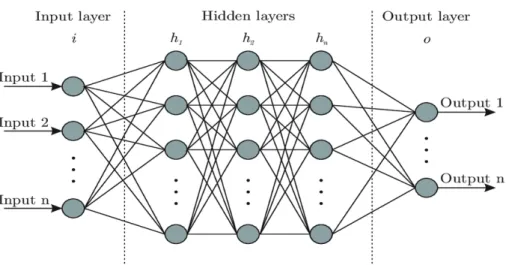
Figure 2.1: Schema of a standard Neural Network, the number of hidden layers is variable. Artificial neural networks (ANNs), commonly called neural networks (NNs), are com-puting systems called so due to the resemblance to human brains where a signal travels between neurons using synapses.

A NN takes an input and produces an output, similarly to traditional programs. The main difference is that the knowledge comes from training on some data, the model changes during such phase until it yields satisfying results and hopefully it can generalize on unseen data of the same kind.

A network, even the more complicated, is made of 3 parts as showed in Figure 2.1: Input Layer where external data is feed into the model

4 2. Theoretical Fundamentals Hidden Layers that are the very heart of the network, this is basically where the

computation takes place

Output Layer the last layer, where the results are expected to be gathered

2.1.1

Neuron

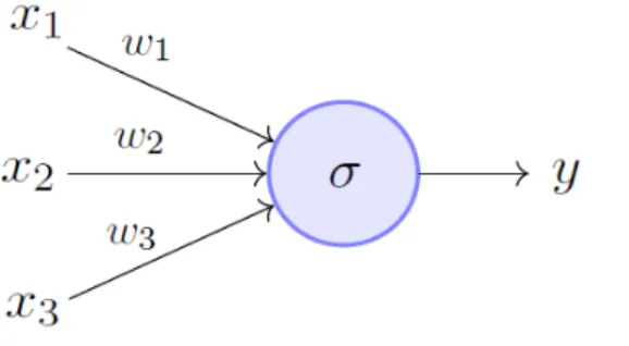
The layers are made of artifical neurons (Figure 2.2), which are minimal logical units. Each neuron outputs the following value:

o = σ((

N

X

i=0

xi∗ wi) + b)

Where x1. . . xN are the outputs of the neurons of the precedent layer, w1. . . wN are

the weights corresponding to each connection related to the output and b is the bias. Then wrapped around this value there is the activation function σ(x), which is a non linear function. The most common activation functions are: ReLU, Sigmoid, TanH and Softmax.

Figure 2.2: An example of Artificial Neuron, in this case there are three inputs xi and

the respective weights wi, then the output y in turn will be an input for the next layer.

2.1.2

Training

The training phase determines the weights and biases of a NN and therefore is crucial for the final outcome. The starting values of the parameters are randomly generated, then they are regulated following some data made of an input and an expected output, also called respectively source and target.

To obtain useful changes we have to evaluate the exactness of the model’s outputs1

against the training samples, so the Loss Function comes in handy. The most basic func-tion is the the Mean Squared Error (MSE) which computes the sum of squared distances between the target values and the predicted ones.

The most common NN learning technique is the Back-Propagation Algorithm, the main idea is to calculate - starting from the output layer going backwards - the value of

2.1 Neural Networks 5 the derivatives of the operations made by neurons with respect to (w.r.t.) weights and

biases (Figure 2.3). From such calculations we can extract how much every parameter2 conditions the output layer and thus if it has to increase or decrease. Those are the directions to follow and an arbitrarily set α, known as Learning Factor, determines how much the parameters change along that direction.

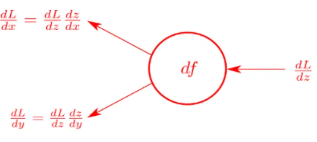
Figure 2.3: A backward pass applied on a neuron, the derivative w.r.t. the neuron output z (dL_dz) is employed to find the derivative w.r.t. the neuron inputs x and y (dL_dx,dL_dy), using the chain rule.

2.1.3

Feed Forward Neural Networks (FFNNs)

A Feed Forward Neural Network is a NN in which the connections between neurons do not form a cycle. The feed forward model is the simplest form of neural network as information is only processed in one direction, data may pass through multiple hidden nodes but it always moves in one direction and never backwards. If every neuron in a layer is connected to every neuron in the following layer the network is called fully connected.

2.1.4

Convolutional Neural Networks (CNNs)

A convolutional neural network, or CNN, is a NN designed for processing structured arrays of data such as images, these type of networks are widely used in the field of computer vision. CNNs contain many convolutional layers stacked on top of each other, each one capable of recognizing more sophisticated shapes. CNNs were primarily used for Extractive Summarization because in that type of task the aim is to generate a sum-mary by ranking sentences, whose performance relies heavily on the quality of sentence features[18].

6 2. Theoretical Fundamentals

2.1.5

Recurrent Neural Networks (RNNs)

A recurrent neural network (RNN) is a type of NN where the output is used as internal state at each time step. This allows to express temporal behavior, as is the networks is working in discrete steps, using each time the previous output. RNNs can use their internal state (memory) to process variable length sequences of inputs.[15]

In fact they were widely used for text generation because of the input and output sequentiality. A RNN can be viewed as many copies of a NN executing in a chain.

2.1.6

Long Short-Term Memory (LSTM)

LSTM[6] is a RNN architecture. The upgrade that this architecture brought compared to vanilla RNNs is computational: standard RNNs cannot bridge more than 5-10 time steps[3] due to that back-propagated error signals tend to either grow or shrink with every time step. This issue is partially addressed in LSTMs because these units allow gradients to flow unchanged. Until the advent of Transformers these kind of networks were the state-of-the-art (SOTA) approach for summarization and NLP in general.

2.1.7

Sequence-to-Sequence Architecture

The most fitting framework for text generation is sequence-to-sequence learning

(seq2seq). Which is about training models to convert sequences from one domain to sequences in another domain. In text summarization the starting domain consists of one or more documents to summarize, also called corpus, and the co-domain is the summary. The basic seq2seq framework for abstractive text summarization is composed of an encoder and a decoder.

Figure 2.4: An example of encoder-decoder architecture, where SOS and EOS respec-tively represent the start and end of a sequence[13].

2.1 Neural Networks 7 The encoder reads a source text, denoted by x = (x1, x2, ..., xI), and transforms it to

hidden states h = (h1, h2, ..., hI); while the decoder takes the last hidden state hI as the

context input along the source text and outputs a summary y = (y1, y2, ..., yO)3. This

framework can be formed by any kind of NN.

2.1.8

Attention

In seq2seq architecture the context vector passed to the decoder turned out to be a bottleneck4, hence in latest models the concept of Attention[1] has been introduced. Attention allows the model to focus more on the relevant parts of the input sequence. An attention model differs from a classic seq2seq model for two reasons:

1. The encoder passes all the hidden states to the decoder, not only the last one. 2. In order to focus on the parts of the input that are relevant to a particular decoding

step, the decoder:

(a) Give each hidden state - which is most associated with a certain word in the input - a score.

(b) Multiply each hidden state by its softmaxed score5_{, doing so it amplifies states}

with high scores and drowns out states with low scores.

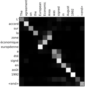
Figure 2.5: The matrix element represents the attention score between the two indexes words, brighter means higher. For example the words accord and agreement have a near one score.

https://jalammar.github.io/visualizing-neural-machine-translation-mechanics-of-seq2seq-models-with-attention/

3_{Where I is the cardinality of the input and O of the output, in our case number of words} 4

8 2. Theoretical Fundamentals The model does not just mindlessly align every output word with the relative input word, it actually learns in the training phase how to align words in that language pair and create meaningful associations. In Figure 2.5 we can see an example of a translation from English to French, it is notable how the attention is reversed for “European Economic Area” because in French is written as “zone ´economique europ´eenne”.

2.2

Transformers

In 2017 Vaswani et al. published “Attention is all you need”[16]. In this paper the Transformer was introduced, a model that innovated NLP field as wasn’t either using RNNs or CNNs, in fact it is based solely on Attention and feed-forward layers.

2.2.1

Structure

Being a type of seq2seq framework a Transformer is made of an encoder and a decoder. The encoder maps an input sequence (x1, ..., xn) to a sequence of continuous

representa-tions6 _{z = (z}

1, ..., zn), also called context vector. Given z, the decoder then generates an

output sequence (y1, ..., ym) one element at a time.

Before being fed both to the encoder and decoder the text sequences pass through an Embedding Layer, its function is to embed text tokens into a vector so that the model can process them. This can be thought of as a lookup table to grab a learned numerical representation of each word. The size of the vector dmodelis a hyperparameter but usually

it would be the length of the longest sentence in the training samples.

After the vector corresponding to a token is obtained, since there is no recurrence or convolution in a Transformer, the information about the position of the word in a sentence needs to be injected. This is done with Positional Encoding, the encodings have the same dimension as the embeddings, so that the two can be summed. There are many choices of positional encodings, learned and fixed. In the paper sine and cosine functions of different frequencies are used:

P E(pos,2i) = sin(pos/100002i/dmodel)

P E(pos,2i+1)= cos(pos/100002i/dmodel)

where pos is the position and i is the dimension. Encoder

An encoder is made of a stack of N7 identical blocks. These can be split in two sub-layers:

6_{An array of floating point numbers}

2.2 Transformers 9

Figure 2.6: Transformer Encoder schema 1. A multi-head self-attention mechanism

2. A simple, fully connected FFNN

A residual connection8 is placed around each of the two sub-layers, followed by layer normalization to reduce training time. Hence the output of each sub-layer is

LayerN orm(x + Sublayer(x))

where Sublayer(x) is the function implemented by the sub-layer itself.

Self-attention will be explained further in the chapter, while the aim of the FFNN layer is to project the attention outputs potentially giving it a richer representation. Decoder

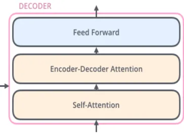
Figure 2.7: Transformer Decoder schema

The decoder is also composed of a stack of N identical blocks. As can be seen in Figure 2.7 the decoder has an extra sub-layer: the Encoder-Decoder Attention, which performs

10 2. Theoretical Fundamentals multi-head attention over the output of the encoder stack. Also the self-attention sub-layer in the decoder stack is modified to prevent attention mechanism from attending to subsequent positions. This masking, combined with fact that the output embeddings are offset by one position, ensures that the predictions for a position can depend only on the known outputs at previous positions. The decoder is capped off with a linear layer that acts as a classifier, and a softmax to get the word probabilities. The decoder is auto-regressive[4], which means the prediction of the yi output token is based on the

(y1, ..., yi−1) previous output tokens and the encoder output, the context. This kind of

text generation is based on the assumption that the probability distribution of a word sequence can be decomposed into the product of conditional next word distributions:

P (y1:t|W ) = T

Y

t=1

P (yt|y1:t−1, W )

where W is the context and T is the length of the word sequence. The decoder’s first input is the <SOS> token, start of sentence, and the token that determines the last step is <EOS>, end of sentence.

The decision of which word to select at a given time-step t is called Decoding Method. The most naive one is Greedy Search, which simply selects the word with the highest probability as its next word:

yt= argmaxyP (y|y1:t−1)

The major drawback of greedy search though is that it misses high probability words hidden behind a low probability word, if we imagine the decision of the next n words as a decision tree the exploration of Greedy Search is not optimal.

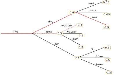
Figure 2.8: An example of generation with num beams = 2

To overcome this Beam Search can be used, the idea is to keep the most likely num beams of hypotheses at each time step and eventually choosing the hypothesis that has the overall highest probability. In Figure 2.8 there is an example of this decoding

2.2 Transformers 11 method. A problem common to both methods is word repetition, to avoid this length

penalty is used. This implementation makes sure that no n-gram appears twice by manually setting the probability of next words that could create an already seen n-gram to 0.

2.2.2

Self-Attention

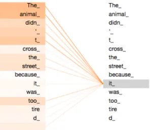
Figure 2.9: In this representation of self attention it’s possible to see the relation of “it” with the other word of the sentence. The attention is strong toward “the animal” because it is what the pronoun (it) refers to.

The attention function used in this architecture is called Scaled Dot-Product Atten-tion. To achieve knowledge on word association three vectors of size dk are extracted

from the input: Query q, Key k, and Value v. These vectors are created by multiply-ing the embeddmultiply-ing of the input word by three matrices that are trainable parameters: WQ, WK and WV. An example to understand the meaning of this mechanism are re-trieval systems. When someone type a query to search for some video on Youtube, the search engine will map the Query against a set of Keys (video title, description etc.) associated with some candidate videos in the database, then it will present you the best matched Values (the videos returned).

Given (x1, ..., xn) as embeddings, calculating self-attention for x1 is done as follows.

The first score would be the dot product of q1 and k1, the second score would be the

dot product of q1 and k2 and so on. These scores are successively scaled9 by

√

dk and

softmaxed, the resulting values sum up to one and represent the correlation between x1

and xi. After we obtained this softmaxed score it is multiplied by the value vector of

12 2. Theoretical Fundamentals associated to x1 can be transcripted as:

o1 = n X i=1 sof tmax(q1√∗ ki dk )vi

In practice the attention function computes simultaneously a set of queries packing them together in the matrix Q, the other vectors are also packed together into K and V:

Attention(Q, K, V ) = sof tmax(QK

T

√ dk

)V

2.2.3

Multi Heading

To obtain an even richer representation of attention Multi-Heading is used. The idea is to train multiple WQ_{, W}K _{and W}V _{matrices to extract different queries, keys and values}

from a single word. Algebraically speaking the embedding is projected in different sub-spaces by each matrix. Doing so the model can focus on more than one position and interpret the sentence in a better way. The number of heads H is a hyperparameter and can be tuned10_.

So H attention outputs for the same word are calculated independently. Then they are concatenated and multiplied by a trainable matrix WO _{to obtain a single vector}

which encapsulates all the information about the original word and can be feed to the FFNN.

2.2.4

Applications of Attention

In a Transformer attention is used differently in each type of layer:

Encoder Self-Attention layers all the keys, values and queries come from the previ-ous layer in the encoder. Each position in the encoder can attend to all positions in the previous layer of the encoder.

Decoder Self-Attention layers allow each position in the decoder to attend to pre-vious positions, this prevents the decoder to peek successive positions to preserve the auto-regressive property. This is implemented by masking out (setting to −∞) all values in the input of the softmax which correspond to illegal connections. Encoder-Decoder Attention layers the queries come from the previous layer while

keys and values come from the output of the encoder. This allows every position in the decoder to use context of all the input sequence.

2.3 Knowledge Distillation (KD) 13

2.2.5

Improvements

The main improvements over RNNs, LSTMs and Convolutional Networks are:

1. Transformers - unlike RNNs - see the entire sentence as a whole, the non-sequen-tiality of processing allows to parallelize the training.

2. Even though LSTMs can capture long term dependencies, attention based models can do it naturally given such mechanism sees all words at once.

3. A self-attention layer connects all positions with a constant number of sequentially executed operations, whereas a recurrent layer requires O(n) sequential operations. In terms of computational complexity, self-attention layers are faster than recurrent layers when the sequence length n is smaller than the representation dimensionality d, which is most often the case with sentence representations used by SOTA seq2seq models. To improve computational performance - for tasks involving very long sequences - self-attention could be restricted to considering only a neighborhood of size r in the input sequence centered around the respective output position, instead of the whole sequence. As side benefit, self-attention could yield more interpretable models.

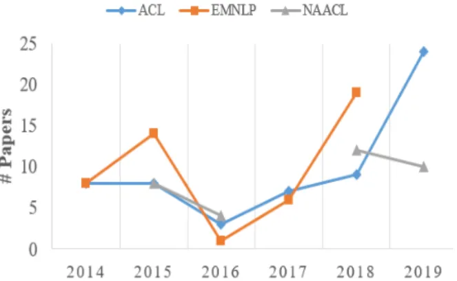
The exceptional contribute to NLP and abstractive summarization in particular can be appreciated in Figure 2.10. From 2017 year of Transformers paper publication -the number of valuable papers on this subject acknowledged by eminent conferences and meetings about NLP increased remarkably11_.

Figure 2.10: In this graph is depicted the trend of the number of Summarization papers accepted from ACL, EMNLP and NAACL during recent years.

2.3

Knowledge Distillation (KD)

Knowledge Distillation is a compression technique12 _{which aims to transfer knowledge}

from a large model to a smaller one without loss of validity. Since recent SOTA

14 2. Theoretical Fundamentals proaches to summarization utilize large pre-trained Transformer models, KD is crucial to make these models available to every platform and not only to devices with high com-putation power. The methods suitable for summarization assume that a student model learns from a larger teacher. However many different distillation methods are proposed by the NLP literature, the ones used in this research will be introduced.

2.3.1

Shrink and Fine-Tune (SFT)

SFT is the most basic method, the idea is to shrink a fine-tuned teacher model to smaller size and re-fine-tune this new student model. Students are initialized by copying an arbitrary number of full decoder layers from the teacher. For example, when creating a student with 4 decoder layers from a teacher with 16 decoder layers, we could copy decoder layers 3, 6, 9 and 12 to the student. Not reducing the encoder layers is due to that decoder is the most useful part to compress while distilling the encoder does not influence too much the inference time13. After initialization, the student model in trained on the same dataset the teacher was fine-tuned on. We assume the dataset is made of a number of pairs (x, y), where x is the source document and y is the target summary. The objective set to train the student is minimizing the standard cross entropy loss function:

L = −

T

X

t=1

log p(yt+1|y1:t, xc)

where T is the length of the target sequence y and p(yt+1|y1:t, xc) is the model’s predicted

probability for the correct word yt+1, given context xc and previous output words y1:t.

2.3.2

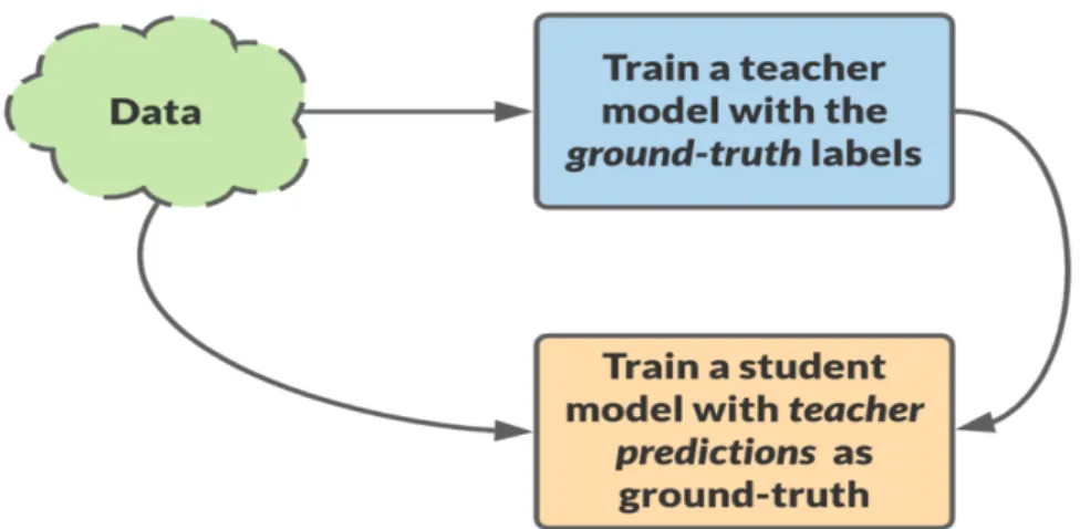
Pseudo-Labeling (PL)

After initializing student models as said before, in Pseudo-Labeling the only difference are the target summaries of the dataset. In the PL method, the target summaries of the dataset are replaced with the teacher’s generated summaries for the source documents. After this the student model is trained like in SFT, minimizing L with the difference that this new pseudo-labeled data is used. So the new function to minimize becomes:

Lpseudo = − T

X

t=1

log p(ˆyt+1|ˆy1:t, xc)

where ˆyi is the i-th token of the generated pseudo-label.

So this method theoretically is an upgrade of the previous one, because the initializa-tion is equal but what differs is the fine-tuning part, which should improve the similarity to the teacher.

2.4 Metrics 15

Figure 2.11: Pseudo-Labeling schema

2.4

Metrics

Evaluation metrics are used to assess the quality of a model, this is essential to ensure that it is operating correctly and optimally. There are a lot of metrics, some are specific to a certain task. A metric common to every model is classification accuracy, which is the ratio of the number of correct predictions to the total number of input samples. But obviously talking about abstractive summarization it is not so useful, since what we expect from the prediction is to maintain the overall meaning but not to use the exact same words of the target summary.

In fact it is quite difficult to find an objective procedure to evaluate the quality of a summary, while for example a classification task is more easy to judge. Serious ques-tions remain concerning the appropriate methods and types of evaluation, indeed there are perplexities over commonly used metric and has been shown that they don’t map very well to human evaluations[9]. Summarization evaluation methods can be broadly classified into two categories:

1. Extrinsic evaluation, when the summary quality is judged by how helpful sum-maries are for a given task.

2. Intrinsic evaluation analyse the summary itself. This category can be again divided into content evaluations, which measure the ability to identify the key topics, and text quality evaluations, which judge the readability, grammar and coherence of automatic summaries.

Text quality is often assessed by human annotators but employing human evaluation for every aspect of the summary is expensive and not practical. The main approach for summary quality determination is the intrinsic content evaluation, which is often done by comparison with an ideal summary, also called gold standard. Now the most used

16 2. Theoretical Fundamentals

2.4.1

BLEU

BLEU (BiLingual Evaluation Understudy) is an algorithm originally developed to mea-sure translation quality, but it is also applicable to summarization. This metric is re-lated to precision, its finality is to compare n-grams14 of a candidate summary with the n-grams of a reference summary and count the number of matches[10]. A normalized ratio is used, so the output is always a number between 0 and 1, this value indicates how similar the candidate text is to the reference text, with values closer to 1 representing more similarity.

The simple precision of o/tc - where o is the number candidate summary n-grams

found in the reference and tc the total number of n-grams in the candidate - could

be misleading. For example considering unigrams15_{, if the candidate is formed by a}

repetition of the same word the precision if such word appears in the reference would be 1. The solution adopted by BLEU is to cap to an arbitrary number omax the number of

effective occurrences of a specific reference n-gram.

To produce a score for the generated summary the modified precision scores for the segments are combined using the geometric mean and multiplied by a brevity penalty to prevent short candidates from receiving a too high score. Let r be the total length of the reference summary, and c the total length of the generated one. If c ≤ r, the brevity penalty, defined to be e(1−r/c), is applied by being multiplied to the modified precision.

2.4.2

ROUGE

ROUGE stands for Recall-Oriented Understudy for Gisting Evaluation[7], it is a set of metrics for evaluating automatic summarization of texts as well as machine translation, which is made of four measures: Rouge-N, Rouge-S, Rouge-W and Rouge-L. Like BLEU it works by comparing a generated summary or translation against a set of refer-ence summaries, the differrefer-ence is that ROUGE is a recall-based measure. The measures used in this research are Rouge-N and Rouge-L.

Rouge-N is an n-gram recall between a candidate summary and a reference sum-mary, it is computed as o/tr where o is the number candidate summary n-grams found

in the reference and tr the total number of n-grams in the reference. So the

differ-ence from BLEU is the denominator, this is more generally the differdiffer-ence between recall and precision metrics. Rouge-L on the other hand measures the longest matching se-quence of words using LCS16_{, such value between two sentences X and Y is defined as}

LCS(X, Y ) An advantage of using LCS is that it does not require consecutive matches but in-sequence matches that reflect sentence level word order. Given a generated

sum-14_{A sequence of n words} 15_{A single word}

2.4 Metrics 17 mary C of lenght lC and a reference summary R of lenght lR, the score is computed as

follows: s = (1 + β 2_)R lcsPlcs Rlcs+ β2Plcs where Rlcs = LCS(C, R) lR Plcs = LCS(C, R) lC and β = Plcs/Rlcs

We notice that s is 1 when R = C while is zero when LCS(X, Y ) = 0. By only awarding credit to sequential unigram matches, Rouge-L also captures sentence level structure in a natural way. Nowadays is the most common metric for summaries evalu-ation.

Chapter 3

Pegasus Model

As said before the recent trend in NLP is pre-training Transformers using self-supervised objectives[11] on large text corpora and use supervised fine-tuning on a smaller dataset only after such operation. This was needed for tasks which use very specific datasets, due to the difficulty of creating these samples, in summarization case documents and summaries pairs. The idea is to train the Transformer on a large amount of text with-out target summaries but pursuing an objective obtained from the text itself and not generated by humans, the objective can vary for every model.

Figure 3.1: In this example of pre-training self objective the phrase “the chef cooked the meal” is masked and the model tries to fill such blanks

For example, the most basic objective is to mask random words from the source document and make them the target of the model during pre-training, as in Figure 3.1. Even if could seem that the model isn’t learning anything task-specific - in this case creating a summary - it is in fact learning how to model the text natural language. As finding the most likely word to fill a masked token is quite similar to fill the next word of the output summary given a context, this kind of objective is called Masked Language Modeling (MLM) and has been used in Google’s BERT[2] pre-training.

Pegasus model has been pre-trained on two large corpora of text:

• C4 (Colossal and Cleaned version of Common Crawl), which consists of text from 350 millions Web-pages (750GB)

20 3. Pegasus Model • HugeNews, a dataset of 1.5 billions articles (3.8TB) collected from news and

news-like websites

The self-supervised objectives will be deepened in the next section. After the pre-training Pegasus has been tested on 12 downstream datasets for summarization, the results of such will be reported in the last section.

3.1

Pre Training Objectives

Figure 3.2: MLM and GSG applied jointly in pre-training, one of the three sentences is replaced by [MASK1] and used as target generation text (GSG). The other two sentences remain in the input, but some tokens are randomly masked by [MASK2]

The pre-training objectives utilized in Pegasus are the aforementioned MLM and a novel method: Gap Sentences Generation (GSG). Given the intended use for abstractive summarization, the objective was thought as similar as possible to generating a summary from the text. So the main idea is to select and mask whole sentences from documents to concatenate the gap-sentences into a pseudo-summary. The corresponding position of each selected gap sentence is replaced by a mask token [MASK_] to inform the model.

To even more closely approximate a summary, the selected sentences are the ones which appear to be important or principal to the document. The approaches considered to set the m sentences to be masked from a document D = {Xi}n are three and can bee

appreciated in Figure 3.3:

• Uniformly select m sentences at random • Select the first m sentences

• Select top-m scored sentences according to ROUGE-1 between the sentence and the rest of the document, si = rouge(xi, D \ {xi}), ∀i

3.2 Results Achieved 21 Using the top scored criteria sentences can be scored independently (Ind) - the previous

seen method - or sequentially (Seq), by greedily maximizing the ROUGE-1 between selected sentences and remaining sentences as:

si = rouge(S ∪ {xi}, D \ (S ∪ {xi})), ∀i

where S is the set of selected sequences. When calculating ROUGE-1 we also consider n-grams as a set (Uniq) instead of double-counting identical n-grams as in the original implementation (Orig). This results in four variants of the principal sentence selection strategy, choosing Ind/Seq and Orig/Uniq options.

Figure 3.3: An example of GSG masked sentences for each approach: Random, Lead

and Ind-Orig.

3.2

Results Achieved

The downstream datasets that Pegasus has been tested on are the following: XSum, CNN/DailyMail, NEWSROOM, Multi-News, Gigaword, arXiv, PubMed, BIGPATENT, WikiHow, Reddit-TIFU, AESLC and BillSum. Each one has different number of samples, different average words per document or summary and different arguments treated in the texts. The paper’s research evaluated lot of different variants but the most important results are the ones for PegasusBASE1, TransformerBASE - which is like PegasusBASE but

without pre-training - and for PegasusLARGE2 both pre-trained on C4 and HugeNews

separately. Both models were pre-trained for 500 thousands steps, the full results can be seen in Figure 3.4. Another difference between the models is the decoding method, for PegasusBASE is Greedy Search, while for PegasusLARGE is Beam Search with length

penalty.

1_{The hyperparameters are, L = 12, H = 768, F = 3072, A = 12, B = 256, where L denotes the}

22 3. Pegasus Model

Figure 3.4: For every model in the columns there are the resulting scores (ROUGE-1/ROUGE-2/ROUGE-L) for each row that corresponds to a downstream dataset

While PegasusBASE exceeded previous SOTA on many datasets, PegasusLARGE

achieved better than SOTA results on all of them with HugeNews pre-training. The improvement from TransformerBASE to PegasusLARGE was more significant on smaller

datasets. ROUGE-2 scores nearly tripled on AESLC and quintupled on Reddit TIFU, this suggests that small datasets benefit more from pre-training than bigger ones.

Also some experiments with low-resource setting has been conducted, the first 10k

training samples3 _{from each dataset has been used to fine-tune Pegasus}

LARGE. The

pre-training consisted in 2000 steps with 256 as batch size with learning rate set to 0.0005. Also adopting such constricting setting previous SOTA has been beat on 6 datasets with only a thousand samples.

Chapter 4

Research

As said before the research question posed is: applying previously seen KD techniques on Pegasus, what is the trade-off between quality of the generated summary and inference time after decreasing the model size? In the following section the main libraries employed in the experiments will be listed. Then in the last section all the steps of the workflow will be explained.

4.1

Libraries

The backbone of this experimentation is PyTorch (PT), a famous open source machine learning library mainly used for Computer Vision and NLP. PT has multiple languages interfaces, but the most common is Python, so that has been used for the research. It has been developed by Facebook’s AI Research lab (FAIR), some of the famous Deep Learn-ing software that use PyTorch are Tesla Autopilot and Uber’s Pyro. The main reason for such choice over TensorFlow (TF) is because this research has been conducted mainly using Hugging Face Transformers (HF), which is a native PyTorch NLP library. Anyway the checkpoints of a model can be easily translated from PT to TF and Transformers is nearly 100% compatible with TF, so this choice is not crucial.

Hugging Face is a company that works mainly on AI chat bots, alongside this ac-tivities HF is developing Transformers: an NLP framework that aims to simplify the deployment of huge models that achieve SOTA in any NLP task (Sentiment Analysis, Question Answering, Text Generation, Summarization,...). The upsides of a unified li-brary made of only three standard classes (models, tokenizers and datasets) are many:

• The carbon footprint is reduced: researchers can share trained models instead of re-training them and practitioners can use the models with less computing power. • High interoperability between PT and TF

24 4. Research Above the three base classes there are two APIs: pipeline() and Trainer(). The first needs only three lines of code to use a model for the related task on any data, while the second quickly fine-tune or train a given model. So Transformers is not intended for building networks (unlike PyTorch or TensorFlow) but to abstract the usage of pre-trained models in NLP field, anyway a model retrieved from Transformers database is a canonical PT/TF model and it’s fully manipulable.

4.2

Workflow

The workflow for experimenting was mainly situated on HF Transformers repository, in fact cloning the repository and installing the required Python packages is enough to download a pre-trained teacher model, initialize a student and train it on a dataset for both STF and PL methods.

4.2.1

Dataset

As said before Pegasus was tested on twelve datasets for summarization, but the most important benchmarks for such task are XSum and CNN/DailyMail. For simplicity and time constraints the KD experiments has been conducted only on Extreme Summariza-tion (XSum) dataset[8].

The XSum dataset has been published in 2018 by Edinburgh NLP, it consists of more than 200.000 BBC articles and accompanying single sentence summaries. The articles range from 2010 to 2017 and cover a wide variety of domains(e.g., News, Politics, Sports, Weather, Technology,...). The split is 90% train, 5% for validation and test, also the data comes already cleaned so there is no need to pre-process.

Figure 4.1: Each row corresponds to a summarization dataset, XSum is in bold. In the first column there are the percentages of novel n-grams found in the target summaries of the dataset, then in the last two columns the R1/R2/RL scores using the baseline methods: LEAD and EXT-ORACLE

The choice of XSum over other datasets comes from the inclination to the abstractive approach, in fact There are 36% novel unigrams in the XSum reference summaries com-pared to 17% in CNN/DailyMail and 23% in NY Times. From the first column of the

4.2 Workflow 25 table in Figure 4.1 we can appreciate how the percentages of novel n-grams in targets is

always more than 18 points higher than other datasets.

In the second column the R1/R2/RL scores - calculated using LEAD1 _generated

sum-maries against the gold references - show that such method performs poorly on XSum, this indicates that such dataset is less biased toward extractive approach. In the third column the same scores are calculated using EXT-ORACLE2_{, they improve for all}

datasets but confirm that XSum is less biased than the others. The extreme summariza-tion dataset is freely downloadable from the Edimburgh NLP repository3, the directory contains a pair of files for each split: a .source file for the articles and a .target file for the summaries.

4.2.2

Student Initialization

The initialization technique was introduced in Section 2.3, so the idea is to copy a reduced number of decoder layers from a pre-trained teacher model, in this case Pegasus. The teacher models are hosted by the HF Transformer library, so the only operation needed to create the student is to run the make_student.py script. Since the experiments are conducted on XSum dataset, the chosen teacher is the model with the weights which will arguably adapt to the task, PegasusXSum4 and not PegasusLARGE, which would be

recommended for customized dataset training. The script needs only three arguments:

teacher the desired teacher model from the Transformers library e the number of encoder layers to copy

d the number of decoder layers to copy

The decision of which layers will be copied for d values less than 16 is decided by a matrix statically allocated in the script. From previous work on distilling BART conducted by HF team[14] is arbitrarily set to copy equally spaced layers, but to always maintain the first and last ones when d is greater than or equal to two.

However different configurations can be tested, probably for values greater than two - for example eight - copying (0, 3, 4, 5, 10, 11, 12, 15) or (0, 1, 2, 3, 12, 13, 14, 15) layers does not change drastically the performance, while there is more difference between (0, 2, 4, 6, 8, 10, 12, 15) and (0, 1, 2, 3, 4, 5, 6, 7, 15). After the script execution a student model with the desired layers is saved in PyTorch format.

1_{A strong lower bound news summarization method that selects the first sentence of a document as}

summary.

2_{An upper bound for extractive models, it creates an oracle summary by selecting the best possible}

set of sentences in the document that gives the highest ROUGE with respect to the gold summary.

26 4. Research

4.2.3

Student Training

For the student training distillation.py script is used, it accepts a large number of op-tional parameters to customize the loop, for example: number of epochs, initial learning rate, max number of words generated for test/validation, batch size for training/valida-tion, and so on. Basically the script execute a normal training loop with a given dataset following the passed arguments.

Finding the best combination of optional parameters is difficult due to the high number of variants and the long execution time. I took some cues from previous works and came up with a shell script to train the XSum students, the most important passed arguments are:

no teacher specifies that the distillation method does not need the teacher model. max source length this set the maximum lenght of input sequences, longer ones will

be truncated and the shorter ones will be padded. For Pegasus it has to be set to 512 because the pre-trained model and the respective tokenizer used such setting. freeze encoder if set make the encoder’s weights unchangeable by the training process, this is used because saves time from the execution and the encoder outputs do not need to be refined.

freeze embeds does the same as freeze_encoder but to the word embeddings, and using the same tokenizer they have to remain the same.

batch size it sets the batch size for training and validation, in this case a batch size of 8 is used for hardware reasons.

gradient accumulation steps sets the number of steps to accumulate before perform-ing a backward pass, it’s set to 32 because this value multiplied by batch_size has to give 256.

val check interval how ofter to run a validation loop, it’s set to 0.1 so there will be ten loops for each epoch.

num beams a parameter for the generation of summaries during training, more beams result in a more deep research in the tree of possible words. It has been set to 4 which is a good compromise between quality and computation time.

early stopping patience sets the number of validation loops needed to early stopping, practically if the average loss of the passed value of consecutive loops doesn’t decrease the training stops before the predetermined time.

4.3 Experiments Settings 27 eval max gen length is the maximum of words generated by each step. It’s set to

35 because the average length of XSum summaries is 24 and after various tests it seemed a good compromise.

length penalty is the length penalty value for Beam Search, it’s set to 0.6 following the default pegasus-xsum parameters.

This will launch the training loop, after every validation loop the metrics are updated and appended to the metrics.json file. The metrics are averaged over the n_val samples of the loop, the most important ones to monitor are loss and ROUGE-2. After the training the test loop will be launched if do_predict is initially passed, this test loop will produce all the basic evaluation metrics, such as: ROUGE-1/2/L, loss and average inference time. This sequence produced the results of the SFT method.

For the PL method the script is used on the resulting model to presumably refine the outputs, the script arguments are similar but the data samples use different target summaries, the ones generated by the teacher. The pseudo-labels can be computed manually or downloaded from the Transformers database, then they will replace the *.target files in the xsum directory.

4.3

Experiments Settings

The defined workflow has been applied changing the initialization phase, in fact the variable that I focused on is the number of decoder layers. So the students created were all Pegasus models with 16 encoder layers but different decoder layers:

• 2 Layers, the layers copied from the teacher are (0, 15) • 4 Layers, the layers copied from the teacher are (0, 5, 10, 15)

• 8 Layers, the layers copied from the teacher are (0, 2, 4, 6, 8, 10, 12, 15)

The different student notation from now on will be 16-n, where n is the number of decoder layers (e.g. student with 2 decoder layers copied is 16-2). For each student the first script reported in subsection 4.2.3 is applied to obtain the SFT results, and after that the PL procedure.

The experiments have been conducted on a GeForce 1060 GTX 6GB GPU, while the maximum epochs have been set to 5 the early stopping sometimes reduced the training time. While the pseudo-labels are pre-generated, if we consider the computing time for generating the summaries from the large model would add 200 hours of computing. The unit of cost is an hour of GPU working, the costs for every distillation method are reported in Table 4.1, considering that the cost for PL comprehends the SFT time

28 4. Research not been conducted on 16-2 student due to the poor results of SFT, so there was no interest on trying to refine.

SFT PL 16-2 14 -16-4 18 28 16-8 9 17

Table 4.1: In each row there is a student model, the first column corresponds to the rough number of hours needed to complete the distillation using SFT method and the second the number of hours for PL

Chapter 5

Results

Figure 5.1: In this plot on the X axis there is the Inference Time measured in milliseconds, while on the Y axis the ROUGE-2 of the models. Every scattered point is labeled with the related student

The full results of the models evaluations on the test samples are visible in the underlying tables, Table 5.1 for the quality metrics and Table 5.2 for the inference time analysis.

From the results it’s notable how the Distillation process didn’t perform well on the 16-2 student, as it reach a low ROUGE-2 score with even more hours of training than 16-8. The 16-8 student operates in nearly half of the time of the baseline decreasing only ˜

3 points in ROUGE-2. On the other hand the 16-4 student has ˜500 ms less of inference time related to 16-8 but small differences in metrics scores, this is probably due to some generation parameter which should be refined. The trade-off seems acceptable, half a second for a slightly better summary is not always worth.

30 5. Results Watching the 16-8 PL results compared to SFT, it is notable a slight increase in metrics, for sure not worth the extra 8 hours of computation. On the other hand for 16-4 the gain is more large, more than one full point in ROUGE-2. From the plot in Figure 5.1 it is appreciable the big leap from distilled models to baseline in Inference Time, while the performances decrease slowly.

SFT PL

16-8 45.04/21.59/36.85 45.10/22.13/37.37 16-4 41.98/19.11/34.51 42.62/20.26/35.49 16-2 35.27/15.61/29.54

-Table 5.1: The rows corresponds to the different students, then in the first column there are the ROUGE-1/ROUGE-2/ROUGE-L scores for the SFT method and in the second column the scores for PL

Inference Time (ms) Speed-up 16-8 2535 1.93 16-4 2084 2.35 16-2 1944 2.52

Table 5.2: The rows corresponds to the different students, then in the first column there is the Inference Time measured in milliseconds (ms) and in the second column the speed-up of the student model related to the baseline inference time (4900)

SFT PL

16-8 -2.17/-2.97/-2.40 -2.11/-2.43/-1.91 16-4 -5.23/-5.45/-4.74 -4.59/-4.30/-3.76 16-2 -11.94/-8.95/-9.71

-Table 5.3: The rows corresponds to the different students, then in the first col-umn there are the decreasing of ROUGE-1/ROUGE-2/ROUGE-L scores related to PegasusLARGE scores1 using SFT and in the second column the same values for PL

Chapter 6

Conclusion

In this thesis I tried to simplify a huge SOTA model for abstractive summarization based on Transformers using two distillation strategies. The overall results were quite good despite the poor hardware and short training time, also the trade-off between inference time and metrics scores seems worth. A model that has to be deployed in any application can’t require a doubled time for a slightly better summary quality. Both KD methods showed acceptable results for the chosen dataset. Said so, further experimentation can be conducted with different initialization or generation settings to try to improve the results.

Bibliography

[1] Dzmitry Bahdanau, Kyunghyun Cho, and Yoshua Bengio. “Neural Machine Trans-lation by Jointly Learning to Align and Translate”. In: (2016). arXiv: 1409.0473. [2] Jacob Devlin et al. “BERT: Pre-training of Deep Bidirectional Transformers for

Language Understanding”. In: (2019). arXiv: 1810.04805.

[3] Felix Gers, J¨urgen Schmidhuber, and Fred Cummins. “Learning to Forget: Contin-ual Prediction with LSTM”. In: Neural computation 12 (Oct. 2000), pp. 2451–71. doi: 10.1162/089976600300015015.

[4] Alex Graves. “Generating Sequences With Recurrent Neural Networks”. In: CoRR abs/1308.0850 (2013). arXiv: 1308.0850.

[5] Geoffrey Hinton, Oriol Vinyals, and Jeff Dean. “Distilling the Knowledge in a Neural Network”. In: (2015). arXiv: 1503.02531.

[6] Sepp Hochreiter and J¨urgen Schmidhuber. “Long Short-term Memory”. In: Neural computation 9 (Dec. 1997), pp. 1735–80. doi: 10.1162/neco.1997.9.8.1735. [7] Chin-Yew Lin. “ROUGE: A Package for Automatic Evaluation of Summaries”. In:

(July 2004), pp. 74–81. url: https://www.aclweb.org/anthology/W04-1013. [8] Shashi Narayan, Shay B. Cohen, and Mirella Lapata. “Don’t Give Me the Details,

Just the Summary! Topic-Aware Convolutional Neural Networks for Extreme Sum-marization”. In: (2018). arXiv: 1808.08745.

[9] Jekaterina Novikova, Amanda Cercas Curry, and Verena Rieser. “Why We Need New Evaluation Metrics for NLG”. In: (Sept. 2017), pp. 2241–2252. doi: 10.18653/ v1/D17-1238.

[10] Kishore Papineni et al. “BLEU: a Method for Automatic Evaluation of Machine Translation”. In: (Oct. 2002). doi: 10.3115/1073083.1073135.

[11] Alec Radford et al. “Language Models are Unsupervised Multitask Learners”. In: (2019).

[12] Colin Raffel et al. “Exploring the Limits of Transfer Learning with a Unified Text-to-Text Transformer”. In: CoRR abs/1910.10683 (2019). arXiv: 1910.10683.

34 BIBLIOGRAPHY [13] Tian Shi et al. “Neural Abstractive Text Summarization with Sequence-to-Sequence

Models”. In: arXiv:1812.02303 (Dec. 2018).

[14] Sam Shleifer and Alexander M. Rush. “Pre-trained Summarization Distillation”. In: (2020). arXiv: 2010.13002.

[15] Ralf C. Staudemeyer and Eric Rothstein Morris. “Understanding LSTM – a tuto-rial into Long Short-Term Memory Recurrent Neural Networks”. In: (Sept. 2019). arXiv: 1909.09586.

[16] Ashish Vaswani et al. “Attention Is All You Need”. In: (June 2017).

[17] Jingqing Zhang et al. “PEGASUS: Pre-training with Extracted Gap-sentences for Abstractive Summarization”. In: CoRR abs/1912.08777 (2019). arXiv: 1912. 08777.

[18] Y. Zhang, M. Er, and M. Pratama. “Extractive document summarization based on convolutional neural networks”. In: IECON 2016 - 42nd Annual Conference of the IEEE Industrial Electronics Society (2016), pp. 918–922.

Credits

I’d like to thank all my family for the continuous support that showed me, my girlfriend which is always source of inspiration for my commitment. Then my friends that are like my second family, the Relator of the thesis Professor Andrea Asperti, who fueled my interest during his course and has introduced me to the world of Deep Learning. Finally to all the colleagues of the degree, everyone has made a little part in helping each other. I thank all of you from my heart.