18
4. SOM-BASED MODELS FOR ESTIMATION OF
CYCLOSTATIONARY PLC CHANNELS
This chapter is organized as follows. First of all, the low-voltage distribution network structure and its main features are outlined. A behavioral model for electrical devices connected to the power grid is proposed, with linear time-varying loads and cyclostationary noise generators. Measurement results from electrical appliances that show this variation are also included. Channel slow-time variation is discussed and a measurement system designed according to it, with signal processing algorithms able to extract cyclic properties, is described. Some representative simulation results of power line channels are also presented. Since short-time variation is also periodic, the channel response can be modelled by a linear periodically time-varying (LPTV) system [5]. A modulation scheme suitable for high-bit-rate transmissions over frequency-selective and slowly time-varying channels is orthogonal frequency-division multiplexing (OFDM). This multi-carrier scheme transforms a frequency-selective channel into a set of multiple flat-frequency fading channels[11],[12]. Thus, equalization of the data with coherent detection amounts simply to normalization by a complex scalar, while the use of non-coherent detection does not require any further equalization. OFDM, however, has its downsides. Loss of the orthogonality between the sub channels is a great problem for OFDM. The commonly used single-tap equalizer assumes that the channel is time-constant in the period between two different channel estimates; thus, it may be unable to fully compensate the loss of sub channel orthogonality due to the cyclic time-variant behaviour of the PLC channel. Then a blind, decision-directed estimation procedure is desired to continuously follow the channel alterations. In this chapter, we propose an adaptive estimation algorithm and the focus is put on tracking the short-time variation of the channel. The proposed scheme is based on a previously proposed SOM decoding scheme[15],[16]. The SOM update rule is modified in order to take into account the dynamic of the channel variation. The proposed method has the SOM as a particular case and is a general decision directed estimation method that reveals to be very effective in the presence of time-varying channels. The performance of the proposed estimation method for power-line channels is evidenced by simulating the transmission over a number of different PLC channels obtained considering a realistic home grid.
19
4.1 CICLOSTATIONARY LOADS
The nonlinear loads can be described as slow time-varying impedances dependent on the mains voltage (230V and 50Hz in Europe). The traditional way to model the communication channel consists in the extraction of analytical or statistical parameters from several configurations. The solution proposed in this thesis adopts a model related to the physical parameters of indoor power lines where only the upper and lower envelopes of the curves expressing the frequency dependence of the impedance are needed. Thus, the proposed method assumes the range of variation of the nonlinear impedances as a known function of the frequency and derives a model of the time-variant impedances considering them as uncertain impedances [9]. These envelopes may be obtained by measurements or by theoretical considerations. This uncertain model of the nonlinear devices permits, by the use of the sensitivity analysis, an efficient determination of the bounds of the responses of the system. It has been shown that the impedances of commonly used domestic devices exhibit a gradual variation of 10%-15% over mains cycle [5]. As a consequence, from the high frequency signal point of view (the Broadband signal) the communication channel is a linear system formed by an interconnection of transmission lines terminated on time varying loads. It was shown that under these circumstances it is possible to consider that, from the high frequency signal point of view, the system is linear but periodically time-varying (LPTV) synchronously with mains. Thus the presence of nonlinear loads produces a cyclic variation of the frequency response of the channel, and this variation is synchronous with the mains [5]. At a given instant, the impedance
z
i
may be approximated by a curve of the family obtained by adding to a linear combination of basis functions of the kind
, , 2 2 , ,2
2
i k P i k P i k i kj
z
j
(Equation 1)
, P i kz
can be viewed as pulse functions of unit height placed at the angular frequency
i kP,
i k2,
i k2, with a width proportional to
i k, . The impedance
, ,
1 i N n P i i i k i k kz
z
z
20
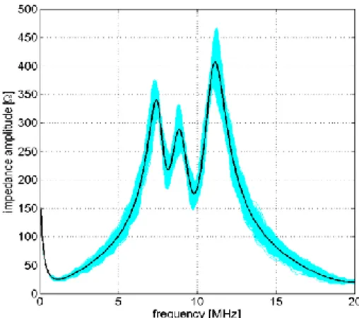
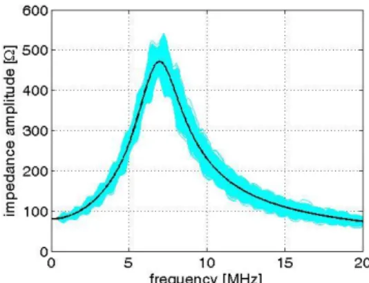
since it can be obtained by the amplitude of the strip at the angular frequency. the expected profile for the impedance of the television, coffee-machine, fun is reported in Fig. 1,2,3.Figure 1: Impedance of a Television
21
Figure 3: Impedance of Fun
4.1.2 Impulsive noise
In order to simulate a PLC channel, the impulsive noise need to be simulated as well, if a rigorous model is required. A classic approach to model impulsive interference is the Middleton Class A noise. This kind of noise model take into account both the background thermal noise and the asynchronous impulsive noise. A frequency domain noise is generated according to the pdf of the noise amplitude
z, the Middleton’s Class A noise probability density function (pdf) of the noise is
given by: 2 0 1 ( ) exp( ), ! 2 2 A m m m m e A z p z m
(Equation 2) with 2 2 , 1 m m A (Equation 3)where A in Eq.2 and in Eq.3 is the impulsive index,
2 2g I
is the GIR
(Gaussian-to-impulsive noise power ratio) with Gaussian noise power
2g
and
impulse noise power
2I
.and
2 2 2g I
22
4.2 In-home PLC Networks
4.2.1 Topology of In-home PLC Networks
The topology of a PLC access network is given by the topology of the low-voltage supply network used as a transmission medium. However, a PLC access network can be organized in different ways (e.g. different position of the base station, network segmentation, etc.), which can influence the network operation as we discuss in 3.2. In this section, we discuss various realizations of PLC access networks and their influence on the network topology and communication organization in the network. We have analyzed network topologies of several PLC access networks realized in various ways. We considered the position of the PLC base station within a low-voltage supply network, network segmentation and interconnection, as well as the in-home PLC networks.
23
Figure 5:Network topology (Network B)
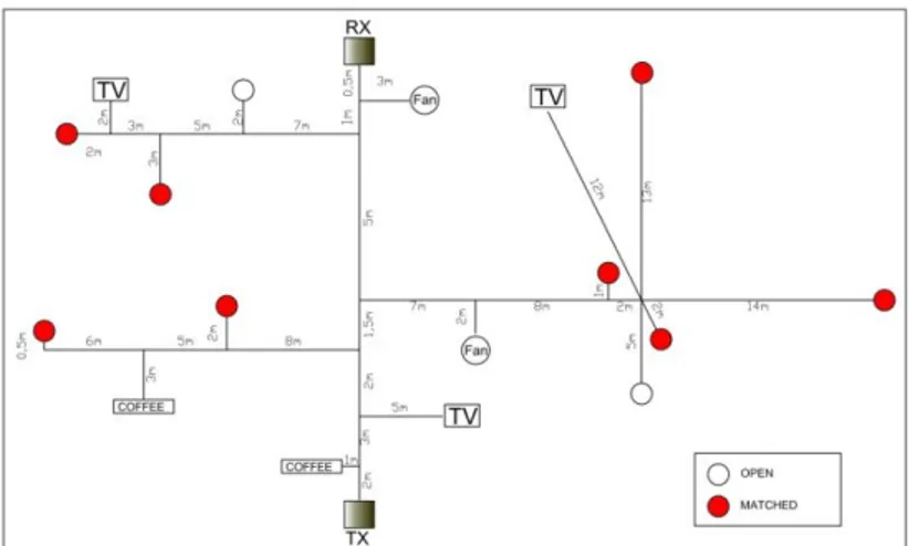
We present in Fig. 4 and in Fig. 5 two possible PLC network configuration covering multiple low voltage networks and including different network elements (open loads, matched loads) and nonlinear devices (the fan, the coffee machine and the TV).
4.2.2 The frequency response
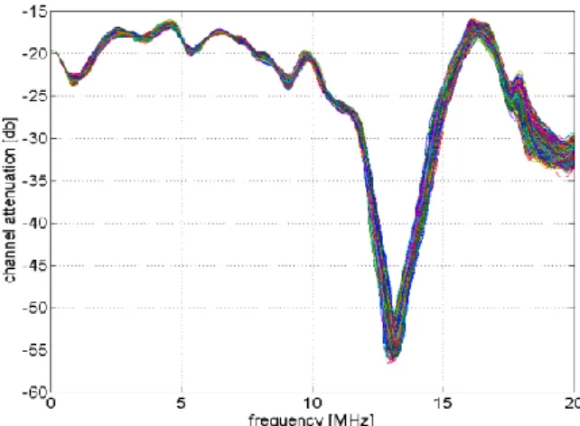
The frequency response of the channel from transmitter (TX) to receiver (RX) is affected by the topology of the low-voltage and by the position of the cyclostationary devices. The varying impedances produce short time variations of the channel that are synchronous with the mains and that can be modeled by assuming a linear periodically time variant frequency response. Under this hypothesis a family of frequency responses of the channel is obtained, for frequencies up to 20 MHz, as shown in Fig. 6 and in Fig. 7. The simulation of the frequency response has been carried out for two different configurations of the loads, which are shown in Fig.4 and in Fig.5. In the network A depicted in Fig. 4 three nonlinear devices (the fan, the coffee machine and the TV) are placed in the direct path from the transmitter to the receiver. The network B in Fig. 5 refers to the same grid but eliminating the cyclostationary loads in the direct path. Figure 6 shows the simulated frequency responses corresponding to network A and Figure 7 the simulated frequency responses corresponding to network B. It can be noticed that the presence of the nonlinear appliances in the direct path between TX and
24
RX contributes to increase the variance of the frequency response of network A, with respect to network B. In fact, the width between lower and upper bound in the frequency response is drastically reduced in Fig. 7 and it is due to the absence of ciclostationary loads in the direct path from transmitter to receiver.Figure 6: Network A, Frequency Response
25
4.3 OFDM multicarrier modulation
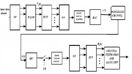
A typical block diagram of an OFDM transmission system is depicted in Fig. 8. and previously discussed in chapter 3
Figure 8: OFDM Transmission system
At the transmitter side, the input data stream is first operated by a serial-to-parallel operation followed QAM modulator. The QAM symbols, which belong to a M-QAM constellation
1, 2,..., M
n
S k Q Q Q , where k indicates the frame and 1... c
n N indicates the subcarrier, are used as the inputs to an IFFT block (modulation) that brings the signal into the time domain. The signal is extended cyclically to form an OFDM frame. This cyclic extension is called the “cyclic prefix”
26
and is inserted by the transmitter in order to remove the inter-symbol interference (ISI) produced by the long impulse response that would otherwise cause degradation of the system performance [11] . After IFFT processing the sequence is again transferred by a parallel-to-serial operation and converted from digital to analog. The power line channel acts as a time-variant frequency selective filter and a source of noise. At the receiver, after a conversion from analog to digital, an FFT block is used to process the received signal. We consider that the inter-symbol interference between two consecutive OFDM frames is completely cancelled by the insertion of a cycle prefix [11]. Assuming that the power line frequency response is constant throughout the k OFDM frame and that synchronization is perfect, the signal at the receiver after the FFT block is expressed by
,n n n n
R t S k W k D k ( Equation 4)
where W kn
are frequency taps of the power line channel and D kn
is the background impulsive noise.4.4 SOM
Self-organizing maps (SOM), invented by Teuvo Kohonen, are artificial neural networks for the visualization of high-dimensional data. It maps complex, nonlinear statistical relationships between high-dimensional data into simple geometric relationships on a low-dimensional display. A self organizing map is therefore characterized by the formation of a topographic map of the input patterns and mantain metric relationships of the primary data elements on the display, it may also be thought to produce some kind of abstractions. These two aspects, visualization and abstraction, occur in a number of complex engineering tasks such as process analysis, machine perception, control, and communication. The term self-organizing map signifies a class of mappings defined by error-theoretic considerations. In practice they result in certain unsupervised, competitive learning processes, computed by simple-looking SOM algorithms.
27
4.4.1 SOM Alghoritm
Figure 9: Self Organizing Map
The basic idea of SOM is simple. The SOM defines a mapping from high dimensional input data space onto a regular two-dimensional array of neurons. Assume that the set of input variables is definable as a real vector x. Each neuron in the SOM array is associated with a parametric real reference vector
,1, ,2,..., ,
l l l l n
m m m m where n denotes the dimension of input vector. The “image” of an input vector x on the SOM array is defined by the decoder function: assuming a general distance measure between x and m, denoted d x m( , ). The neurons of the map are connected to adjacent neurons by a neighborhoods relation, which dictates the topology, or structure, of the map. Our task is to define the m, in such a way that the mapping is ordered and descriptive of the distribution of x. One may try to determine the m, by an optimization process, following the idea of the classical vector quantization (VQ) . In the basic SOM algorithm, the topology and
the number of neurons remain fixed from the beginning. The learning process of the SOM goes as follow:
28
1. Let p x
be the probability density function of x , or x one sample vector drawn from the input data set and let m , be the codebook vector that is closest to x in the signal space, i.e., d x m( , ) is smallest. (e.g using the common Euclidean distance measure or the average expected quantization error function)2. The set of values
m that minimizesd x m( , )is the solution of the VQ problem, and the signal space is mapped onto the set of codebook vectors. However, the indexing of these values can be made in an arbitrary way, whereby this mapping is still unordered. The BMU itself as well as its topological neighbors are moved closer to the input vector in the input space, the input vector attracts them. The magnitude of the attraction is governed by the learning rate. As the learning proceeds and new input vectors are given to the map, the learning rate gradually decreases to zero according to the specified learning rate function type. Along with the learning rate, the neighborhoods radius decreases as well. The approximate optimization algorithm is then
, 1 , l l c l l c m t t x t m t i N t m t m t i N t (Equation 5)where
t is a small positive scalar factor that determines the size of the gradient step at time t. This is a classical and thoroughly investigated approach. If the function
t is chosen suitably, the sequence of the m t
will always converge to the set of values
mt that approximates the solution for
m . Many different SOMalgorithms can be represented by equation 5.
3. The steps 1 and 2 together constitute a single training step and they are repeated until the training ends.
After the SOM has been trained it is important to know whether it has properly adapted itself to the training data. Because it is obvious that one optimal map for the given input data must exist, several map quality measures have been proposed.
29
4.5 Proposed estimation method
The use of the SOM for filtering and decoding the received M-QAM symbols in a OFDM system for power-line channels has been originally proposed by the authors in [15] and [16], and it is based on the use of one model vector (neuron), that is a complex number,
1, , M
n n
C C for each M-QAM symbol of the subcarrier n . Each neuron i
n
C takes trace of the center of the correspondent symbol cluster. When the symbolR kn
of (4) is received, the nearest neuron in the Euclidean norm (called best matching unit BMU) is selected:
1 arg min{ i }. n n i M c R k C k ( Equation 6)Hence the correspondent transmitted symbol is estimated as Sˆn
k Qc. After that, the positions of neurons are adjusted with:
1
, i i i n n ci n n C k C k h R k C k (Equation 7) where 1 , 1 1 , ci i c h h i M i c 30
and is a fixed step size. The BMU is moved in the direction of the received symbol, while the other model vectors are slightly modified. In order to have coherent detection, the neurons have to be initialized with the channel information. Given the initial channel estimates Wn
0 ,n1...Nc, the neurons are initializedaccording to
0
0 , 1 , 1 .i i
n n c
C Q W i M n N ( Equation 8)
At the successive OFDM frames, neurons will be blindly adjusted according to (3), thus this method is a decision directed estimation strategy. The drawback of the rule (7) is that in the case of a continuous channel migration, such as in a cyclostationary power-line channel, a constant gap will remain between the moving symbols and the follower neurons. In fact, the SOM rule acts as a first order low pass discrete filter of the received symbols (4), where the cut-off frequency is related to the step size . It is known that a first order filter is not capable to have zero error to an input with constant velocity. Another drawback is that the background noise will be filtered by a first order low pass filter, whereas a higher order filtering action may be desired. For these reasons we introduce a new method where we propose a modification of the basic SOM update rule in order to implement an arbitrary filter dynamic between the received symbols and the model vectors. For instance, a filter with a second order dynamic can be properly designed in order to have a better tracking capability than equation (7), or in order to have a better filtering action on the background noise. Hence, we propose to design a discrete linear filter of order N.
1 1 2 1 1 2 1 ... ( ) .... N N N N N N b z b z b G z z a z a . (Equation 9)
Then the dynamic G z( ) is implemented in the SOM by the following discrete equation
31
,1 1 2 , ,1 , 1 2 1 . i i n n n i N i i N N n n N n C k b R k b R k b R k a C k a C k (Equation 10) Where
,1 ,1 ,1 , , , 1 , ,1 ,1 ,1 , , , 1 , 1 1 , 1 1 i i i i n n ci n n i p i p i p i p n n ci n n i i i n n ci n n i p i p i p i p n n ci n n C k C k h C k C k C k C k h C k C k R k R k h R k R k R k R k h R k R k (Equation 11)and p2 N. The parameter hci is defined as in (7) and the BMU is calculated as in (6). Equation (10) implements a one-step time shift of the variables of the filter only for the BMU, while it keeps the variables of the other neurons almost unchanged, so that only the BMU is updated by (9). This model gives a general framework to define different filtering strategies, where the basic SOM is a particular case. In most cases, the design of G z( ) is accomplished by designing a low pass filter, and the main parameter is the cut-off frequency. Examples of possible choices of G z( ) and the benefits obtained in the tracking and the decoding of the symbols are described in the following section.
32
4.6 Transmission simulations
In this section we simulate the transmission in the link considering the two different channels shown in Fig. 4. The reported results show general trends observed by the authors in several simulations. We have simulated the transmission of random data by using a OFDM modulation with a number of Nc512 subcarriers. Each subcarrier is modulated with a gray-coded 16-QAM symbol constellation and the transmitted power is uniformly distributed between subcarriers. We simulate different conditions of signal to noise ratio by varying the total transmitted power and considering a fixed noise condition. We can reasonably assume that the frequency response is constant during the duration of one OFDM frame. A new response is considered at each frame, which belongs to the family of the cyclostationary responses described in the previous section. The variation between two consecutive channels is small in order to simulate a smooth continuous migration of the channel. At the receiver we simulate three different estimation methods. In the method 0 we consider a constant estimation W of the channel at n each carrier n , equal to its average value along one mains cycle. Then we initialize the neurons as
0 , 1 , 1i i
n n c
C Q W i M n N (Equation 12)
and the neuron positions are kept constant:
1
0i i
n n
33
Figure 10: Global bit error rates of channel A
34
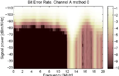
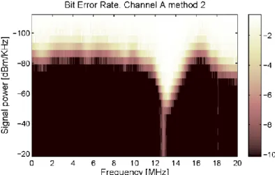
This method is equivalent to a pilot aided method that accomplishes an initial supervised estimation W and then consider the channel constant, thus neglecting n the cyclostationary effect. In the case of a stationary channel (in the absence of the cyclostationary phenomenon) the method 0 is equivalent to consider perfect channel estimation. In the method 1 we consider the basic SOM decision directed estimation. In particular this can be obtained as a particular case of the proposed method by taking a filter of order N1 and considering a filter with the following numerator and denominator coefficients b[ ,0]; a[1,(1)]. In the method 2 we consider a filter of order N2, in particular we consider a low pass discrete Butterworth filter [6]. The cut-off frequency of the filter in method 2 is selected in order to be equal to the cut-off frequency of the first order filter of method 1, which is related to the step size . Acceptable values of the step size vary in the interval [0.01,0.1], and the choice of has to be carried out as a trade-off between a better noise filtering action (smaller values of ) or a stronger tracking capability (higher values of ). However in this simulation we are interested in the comparison between methods 1 and 2 for fixed (filter bandwidth), so we take a value of fixed for all the simulations. The choice of the Butterworth filter is dictated by its good proprieties both in the frequency domain (the flat band up to the cut-off frequency), and in the time domain (optimal damping ratio). The flat band assures that the filter will not produce noise amplification, and the good transient response assures a good tracking ability of the time varying channel. For each simulated PLC channel we calculate a global bit error rate BER and also a BER at each subcarrier. Figure 5 shows the global BERs obtained in the two channels. In both cases a similar trend is observable: the BER obtained with three methods has similar decrease up to a signal power, after which the BER of method 0 remain steady at its minimum, while the two decision-directed methods can reach lower values. For channel A the methods 1 and 2 also reach a BER floor, where method 2 has better results. This can be explained by the fact that up to this signal power the noise is the predominant cause of error, and the three methods have a similar behavior, while for high signal to noise ratios the only source of error is the cyclostationary variation of the channel. In this condition the method 0 that makes the hypothesis of a constant channel reveals its limits, while the decision directed methods, that blindly follow the migration of the symbols, significantly reduce the error. This can be seen also by the fact that the height of the BER floor of the method 0 for high signal powers, increases if the channel has stronger cyclostationary behavior. In fact the BER floor of the method 0 decreases from channel A to channel B. These results clearly show that in order to fully exploit the channel capacity , the cyclostationary effect cannot be neglected and good channel estimate methods must be adopted for an efficient equalization. Figure 6 shows the BER of the channel A . The color-bar indicates the base 10 exponent of the relative BER. It is clear that for method 0, at high signal powers, the error is generated only in those frequencies where the width of the cyclostationary variation is high. For the methods 1 and 2 the BER in those frequencies is strongly reduced. Moreover, the method 2 shows a better performance of method 1 for channel A. In particular, the advantage of method 2 over method 1 is clearer at the frequencies where the cyclostationary effect is strong. In fact, in the BER calculation for channel A, there35
are some carriers where method 1 reveals a BER floor while the method 2 reaches a zero BER. For instance, there is a line near 14.8 MHz in the BER of method 1 which is not present in the BER of method 2. This line has been marked and can be easily observed in Fig. 6. The benefits on the global BER of method 2 over method 1 depend on the number of carriers where the cyclostationary effect is significant. Hence the benefits of the proposed method, based on a second order filter, are clearly established on the carriers where the channel variation is important, demonstrating the superior ability of the proposed method to follow the cyclostationary channel variations.Figure 12: BER at each carrier on channel A for method 0
36
Figure 14:BER at each carrier on channel A for method 2
4.7 Consideration
Low-voltage networks were designed only for energy distribution to households and a wide range of devices and appliances are either switched on or off at any location and at any time. This variation in the network charge leads to strong fluctuation of the medium impedance. These impedance fluctuations and discontinuity lead to multipath behavior of the PLC channel, making its utilization for the information transmission more delicate. Beside these channel impairments, the noise present in the PLC environment makes the reception of error-free communication signal more difficult. The noise in PLC networks is diverse and is described as the superposition of five additive noise types, that are categorized into two main classes – on the one hand is the background noise, which remains stationary over long time intervals, and on the other is the impulsive noise, which consists of the principle obstacle for a free data transmission, because of its relative high intensity. This impulsive noise results in error bursts, whose duration can exceed the limit to be detected and corrected usually by used error correcting codes. Therefore, the impulsive noise in PLC networks has to be represented in appropriate disturbance models. A novel decision directed estimation algorithm for OFDM systems has been introduced. This method generalizes a previous proposed estimation scheme based on a SOM neural network , introducing the possibility to implement the dynamic of a filter, arbitrarily designed, inside the SOM. This leads to a better estimation and tracking of a time variant frequency response. The use of a filter with a second order dynamic reveals a better BER in the