LHC Bounds on Large Extra Dimensions

1

Università di Pisa

Facoltà di Scienze Matematiche, Fisiche e Naturali

Corso di Laurea Magistrale in Fisica

Elaborato Finale

LHC Bounds on Large Extra Dimensions

Candidato

Giorgio Busoni

Chiarissimo Prof. A. Strumia

Relatore

2

This work is dedicated to my family and to those that really love me. To my father Marco, who has always supported and encouraged me in my choices; to my mother Alessandra, maybe the person who loves me most in the world; to my brother, Dario, to my grandfather Alberto, to my grandparents Luciano and Lidia, who are no longer here, but who would have liked to be here, and last, but not the least, but particularly it is dedicated, to my grandmother Greta, who has always helped me in every step of my life with love, and without whom probably I wouldn’t be who I am.

3

Index

Index ... 3

0 Premises ... 7

0.4 Values of coupling constants ... 8

1 Introduction ... 9

1.1 Hierarchy Problem ... 9

1.1.1 Planck scale ... 9

1.1.2 Higgs Boson mass ... 9

1.1.3 Zero-point energy ... 9

1.1.4 Super-symmetry Solution ...10

1.1.5 Models with additional dimensions ...10

1.1.6 The ADD/GOD model and the Large Extra Dimensions ...11

2 Standard Model... 13

2.1 Standard Model and the Yang-Mills Lagrangian ...13

2.1.1 Gauge invariant definitions ...13

2.1.2 Boson Fields ...14

2.1.3 Fermion Fields ...15

2.1.4 Higgs Field Lagrangian ...16

2.1.5 Higgs’s and fermions’s couplings Lagrangian ...17

2.2 Feynman Rules for the Standard Model ...18

2.2.1 How to obtain Feynman Rules for the propagators ...18

2.2.2 Feynman Rules for the propagators, Standard Model ...18

2.2.3 How to obtain Feynman Rules for vertices ...19

2.2.4 Feynman Rules for vertices, Standard Model ...19

2.3 Running Coupling Constant ...20

2.4 Two body processes general Kinematics ...21

2.4.1 Degrees of freedom ...21

2.4.2 Mandelstam variables ...21

4

2.5 Cross section calculation of elementary processes between partons ...24

2.5.1 𝒈𝒈 → 𝒈𝒈 ...24 2.5.2 𝒈𝒈 → 𝒒𝒒...24 2.5.3 𝒒𝒒 → 𝒈𝒈...24 2.5.4 𝒈𝒒 → 𝒈𝒒...25 2.5.5 𝒒𝒒 → 𝒒𝒒 ...25 2.5.6 𝒒𝒒 → 𝒒𝒒 ...25 2.5.7 𝒒𝒒 → 𝒒′𝒒′ ...25 2.5.8 𝒒𝒒′ → 𝒒𝒒′ ...25

2.6 Deep Inelastic Scattering ...26

2.6.1 Useful variables ...26

2.6.2 Bjorken’s Scaling...27

2.7 Parton Distribution Functions ...27

2.8 Proton-Proton processes ...28

3 Gravity Interactions ... 30

3.1 Einstein’s Equation ...30

3.1.1 Kaluza-Klein modes ...30

3.1.2 Physical Fields and Gauge-dependent Fields ...31

3.1.3 Identification of the Particles ...33

3.2 Gravitational Lagrangian ...34

3.3 Feynman rules ...34

3.3.1 Feynman Rules for propagators ...34

3.3.2 Feynman Rules for vertices ...35

3.4 Real Graviton Production ...36

3.4.1 Modes density ...36

3.4.2 Real Graviton production cross sections ...36

3.4.3 Expected results ...38

3.5 Virtual Graviton Exchange ...38

3.5.1 Scattering amplitudes ...38

3.5.2 Relevant processes Cross sections ...38

3.5.3 Expected results ...40

3.6 Limits on the application of perturbation theory ...41

4 Experimental Parameters ... 42

5

4.2 Hadron Colliders Kinematics ...42

4.2.1 𝑪𝒐𝑴 Frame ...42

4.2.2 Variables for integration over the 𝑷𝑫𝑭 ...43

4.2.3 Transverse momenta and Azimuthal Angle ...43

4.2.4 Rapidity and Pseudo-rapidity ...43

4.2.5 Lego Plot and jet resolution ...44

4.3 Machine Diagram ...44

4.3.1 Detectors ...44

4.3.2 Decay length and direct and indirect measurements ...45

4.3.3 Indirect measurements...47

4.3.4 Triggering ...47

4.4 Experimental cuts...48

4.4.1 Real Graviton production cuts ...48

4.4.2 Virtual Graviton Exchange cuts ...48

5 Simulations with Mathematica ... 49

5.1 MonteCarlo integration method ...49

5.1.1 Numerical Integration...49

5.1.2 MonteCarlo: Sampling method ...49

5.1.3 MonteCarlo: Hit and miss method ...50

5.1.4 MonteCarlo Integration accuracy: sampling method...50

5.1.5 MonteCarlo Integration accuracy: Hit and miss method ...51

5.1.6 Comparing integration with and without changing variables ...52

5.2 Implementation in Mathematica ...53

5.2.1 Choosing the integration variables...53

5.2.2 Generating events ...53

5.2.3 Implementing cuts ...54

5.2.4 Memorizing points ...54

5.2.5 Calculating cross section ...54

5.2.6 Important precautions ...54

5.2.7 Used Approximations ...54

5.3 Testing the program with the Standard Model ...55

6 Results ... 57

6.1 Virtual Graviton Exchange ...57

6

6.3 Cross section dependence on Graviton’s mass cut-off ...59

6.4 Bounds on 𝑴𝑫 and 𝚲, 2010 data ...60

6.5 Bounds on 𝑴𝑫 and 𝚲, 2011 data ...63

6.6 Conclusions ...65

7 Appendix ... 66

7.1 Calculation of the gravitational field in the Large Extra Dimensions with the images method ...66

7.2 Parton Distribution Functions from H1 and HERA data ...67

7.3 Used functions ...68

7.3.1 Functions 𝑭 ...68

7.3.2 Functions 𝓕 ...68

7.4 Comparison between Numerical and MonteCarlo Integration ...68

7.4.1 Numerical Integrations comparison source code (fixed number of points) ...69

7.4.2 MonteCarlo comparison source code ...70

7.4.3 Numerical Integration comparison source code (variable number of points) ...71

References ... 72

7

0 Premises

0.1 Notation

Greek indices have been used for four-vectors, and run from 0 to 3.

Four-vectors may be written separating the time component from the space components 𝑋𝜇_{= �𝑋}0_{, 𝑋⃗�.}

The quadri-dimensional metric is (+, −, −, −).

Indices 𝑗, 𝑘, 𝑙, 𝑚 run over the Extra-dimensions, therefore their values run from 4 to 3 + 𝛿. Indices 𝑎, 𝑏, 𝑐, 𝑑 run over all dimensions, and so their values run from 0 to 3 + 𝛿.

As color indices, 𝑎, 𝑏, 𝑐 or 𝑖, 𝑗, 𝑘 have been used.

The subscript/superscript 𝐹 stands for a generic fermion, 𝐵 for a boson, 𝑄 for a quark, 𝑔 for a gluon. If a graviton is present in a vertex, indices 𝜇, 𝜈 are to be assigned to the graviton, while 𝛼, 𝛽, 𝛾, if present, refer to Photons or Gluons.

All the charges are expressed as multiples of the elementary charge, therefore they are dimensionless numbers.

Means of quantities have been indicated with 〈 〉, or, where this couldn’t cause confusion, with � . References have been indicated with a number in square brackets [𝑛𝑢𝑚𝑏𝑒𝑟]

0.2 Natural Units

Natural units have been used, in this system

ℏ = 𝑐 = 1 (0.2.1) The use of natural units simplifies a lot the writing of the formulas.

All energies are measured, as usually done in Particle Physics, in 𝐺𝑒𝑉, and, thanks to the fact that 𝑐 = 1, masses and momenta are measured in 𝐺𝑒𝑉 as well.

The value of 𝐺, in this measurement system, is expressed in 𝐺𝑒𝑉−2 _{and is}

𝐺 = 6.7087 ∙ 10−39_𝐺𝑒𝑉−2 _(0.2.2)

0.3 Conversion factors

The use of natural units makes the 𝑓𝑚 be the inverse of 𝐺𝑒𝑉, when converting from one of these units to the other, we have to remember that

1 = ℏ𝑐 = 197.3𝑀𝑒𝑉 ∙ 𝑓𝑚 (0.3.1) Therefore we obtain the following conversion factors

8

1𝐺𝑒𝑉−1_{= 10}−3_𝑀𝑒𝑉−1_{= 10}−3_𝑀𝑒𝑉−1_{∙ 197.3𝑀𝑒𝑉 ∙ 𝑓𝑚 = 0.1973𝑓𝑚 (0.3.2)}

For the cross sections we need square of lengths (areas)

1𝐺𝑒𝑉−2_{= 10}−6_𝑀𝑒𝑉−2_{∙ (197.3𝑀𝑒𝑉 ∙ 𝑓𝑚)}2_{= 0.03893𝑓𝑚}2 _(0.3.3)

If we want to measure cross sections in picobarn, that is

1𝑏 = 10−28_𝑚2_{→ 1𝑝𝑏 = 10}−40_𝑚2_{= 10}−10_𝑓𝑚2 _(0.3.4)

The conversion factor that we need is

1𝐺𝑒𝑉−2_{= 0.03893𝑓𝑚}2_{∙ 10}10 𝑝𝑏

𝑓𝑚2= 3.893 ∙ 108𝑝𝑏 (0.3.5)

0.4 Values of coupling constants

The values of the coupling constants for the standard model are:

𝑔 = 0.652 𝑔′_{= 0.357 𝑒 = 0.09173 𝛼 =} 𝑒2

4𝜋 = 0.0073 (0.4.1) while 𝑔𝑆 and so 𝛼𝑆=𝑔𝑆

2

4𝜋 are strongly dependent on the energy value at which the process takes place

9

1 Introduction

1.1 Hierarchy Problem

In physics we call “Hierarchy problem” the fact that some fundamental constants in a Lagrangian (coupling constants or masses) are totally different from their experimental values. This may happen because the measured values are not the bare ones of the Lagrangian, but the renormalized ones. Radiative corrections usually cause small corrections of the bare values, but sometimes there might be cancellations between fundamental quantities and radiative corrections.

1.1.1 Planck scale

Combining the fundamental constants 𝑐, 𝐺, ℏ, we may obtain 4 quantities with the dimensions of length, time, mass, and energy. They are

𝑙𝑝 = �ℏ𝐺_𝑐3 ≅ 1,1616 ∙ 10−35𝑚 (1.1.1) 𝑡𝑝 = �ℏ𝐺_𝑐5 ≅ 5,391 ∙ 10−44𝑠 (1.1.2) 𝑀𝑝 = �ℏ𝑐_𝐺 ≅ 1,2209 ∙ 1019𝐺𝑒𝑉_𝑐2 ≅ 21.76 𝜇𝑔 (1.1.3) 𝐸𝑝 = �ℏ𝑐 5 𝐺 ≅ 1,2209 ∙ 1019𝐺𝑒𝑉 ≅ 1.1956 𝐺𝐽 (1.1.4)

Gravity should became important when we get close to these values, that is on very small scales of length , that is on very large energy scales. These scales are very far from the ones probed experimentally.

1.1.2 Higgs Boson mass

In the Standard Model, the “Hierarchy Problem” is about the Higgs Boson mass. Its value is considered to be between 100𝐺𝑒𝑉 and 1𝑇𝑒𝑉. We would expect this value to be, because of quantum corrections, much larger. Radiative divergences are usually power-law, and therefore they are proportional to a power of Λ𝑐𝑢𝑡𝑜𝑓𝑓, the maximum energy for the validity of the standard model. In the Standard Model, assuming that

there are no changes in the physical laws up to the grand unification with the gravitational force, that should take place at Planck scale, Λ𝑐𝑢𝑡𝑜𝑓𝑓 should then be equal to the Planck energy, that is 1019𝐺𝑒𝑉, and

therefore we would expect the Higgs Boson mass to be the same order of magnitude, unless opportune cancellations could reduce its value of 17 orders of magnitude.

1.1.3 Zero-point energy

When we quantize a field, for example a scalar field, we find out that the energy density of the vacuum receives an infinite contribution from the zero-point energy of the oscillations modes. If we put a cut-off Λ𝑐𝑢𝑡𝑜𝑓𝑓, this energy density is about

10

⟨0|𝐻|0⟩~Λ4𝑐𝑢𝑡𝑜𝑓𝑓 (1.1.5)

Fermion fields give a similar contribution, but of opposite sign. Spontaneous symmetry breaking contributes with another term

⟨0|𝐻|0⟩~ − 𝑎𝑣4 _(1.1.6)

where 𝑣 is the expectation value of the field and 𝑎 is a positive constant.

In strong and electroweak interactions, this zero-point energy shift cannot be observed, as only differences in energy can be measured. Anyway, as the source of gravitational field is the energy-momentum tensor, energy couples with gravity, and therefore zero-point energy should contribute to the gravitational field as source term in Einstein’s equation. A zero-point energy density 𝜆 contributes to Einstein’s equation with a source term 𝜆𝑔𝜇𝜈_{; this term has the form of the cosmological constant term in Einstein’s equation. We may}

therefore think that a cosmological constant in Einstein’s equation may be due to a non-zero zero-point energy, but the two parameters have completely different values, indeed zero-point energy density is, as stated above, about Λ4𝑐𝑢𝑡𝑜𝑓𝑓, while the observed value of the cosmological constant is

𝜆 ≈10−30𝑔

𝑐𝑚3 ~(2.3 ∙ 10−12𝐺𝑒𝑉)4 (1.1.7)

Therefore the two values differ of 120 orders of magnitude.

1.1.4 Super-symmetry Solution

A way of solving the Higgs mass problem is hypothesizing the existence of a super-symmetry, that is the existence, for each boson, of a fermion with opportune mass and quantum numbers to cancel exactly the radiative contribution of the boson at every renormalization order; and vice-versa, the existence, for each fermion, of a boson with the same properties. This would cancel all the radiative contributions to the Higgs mass. The problem is that none of such particle partners have been found yet, and this raises questions on their effective existence.

Fig. 1.1. Left: diagram of a radiative contribution of a fermion. Right, diagram of a contribution due to a boson.

1.1.5 Models with additional dimensions

In a world with 3+1 dimensions, we can find the gravitational field in the case of a point particle using the Gauss’s Theorem

𝑔(𝑟⃗) = −𝐺𝑚_𝑟2 𝑟̂ = − 𝑚

𝑀𝑃2𝑟2𝑟̂ (1.1.8)

We assume now that there are 𝛿 additional dimensions where the gravity is free to propagate. The previous law would change to

𝑔(𝑟⃗) = −𝐺′𝑚 𝑟2+𝛿𝑟̂ = −

𝑚

11

where 𝐺′ and 𝑀𝐷 are new constants. Unfortunately the modified law would wouldn’t be in agreement with

experimental data, in fact the law

𝑔(𝑟⃗) ∝ −_𝑟1₂𝑟̂ (1.1.10) has been verified for many orders of magnitude, up to 1𝑚𝑚.

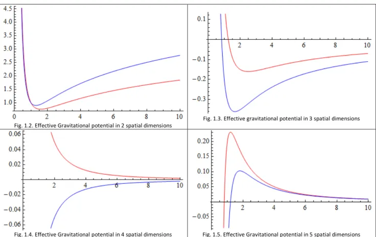
Moreover, even without comparing with experimental data, we find that the effective potential of a two body problem, for a number of dimensions greater than 4, would not have a minimum and therefore there would be no stable orbits.

Fig. 1.2. Effective Gravitational potential in 2 spatial dimensions Fig. 1.3. Effective gravitational potential in 3 spatial dimensions

Fig. 1.4. Effective Gravitational potential in 4 spatial dimensions Fig. 1.5. Effective Gravitational potential in 5 spatial dimensions

Therefore additional dimensions, if they exist, cannot be infinite.

1.1.6 The ADD/GOD model and the Large Extra Dimensions

We assume now that additional dimensions are compact and have a limited radius 𝑅 (for example a 2-sphere or a 2-torus with zero internal radius).

In this case, for small distances 𝑟 ≪ 𝑅 law 1.1.9 would apply, while for larger distances 𝑟 ≫ 𝑅 the classical gravitational field would be*

𝑔(𝑟⃗) = − 𝑚

𝑀_𝐷2+𝛿_𝑟2_𝑅𝛿𝑟̂ (1.1.11)

because gravity could not propagate for more than a distance 𝑅 in the additional dimensions, as those have a finite small radius.

12 From that law we derive the relation

1

𝐺 = 𝑀𝑃𝑙2~𝑀𝐷2+𝛿𝑅𝛿 (1.1.12)

This relation would explain the large size of the Planck mass: it is not a new fundamental energy scale, and its largeness is due to the large radius of the additional dimensions.

Assuming that the only important energy scale is 𝑀𝐸𝑊~𝑀𝐷, maximum energy for the validity of the

Standard Model (and of the same order of the Higgs mass), we obtain

𝑅~ � 𝑀𝑃𝑙2 𝑀_𝐸𝑊2+𝛿� 1 𝛿 𝑓𝑚 = 1030𝛿 −17_{𝑐𝑚 ∙ �}1𝑇𝑒𝑉 𝑀𝐸𝑊� 1+2𝑛 (1.1.13)

𝛿 = 1 would imply 𝑅 = 1013_{𝑐𝑚 and therefore it would imply changes on scales of length at which gravity}

has been verified changing with the rule ∝ −_𝑟12, and so 𝛿 = 1 is not a possible choice. On the contrary, for

𝛿 ≥ 2 and 𝑀𝐸𝑊~1 𝑇𝑒𝑉 we obtain 𝑅 ≤ 0.1 𝑚𝑚 and therefore scales of length at which gravity has not

been experimentally probed yet, and so this new theory may apply.

We must remember that, if gravity has been tested only up to scales of 1𝑚𝑚, strong and electroweak interactions have been probed up to scales of 1𝑓𝑚, and therefore it is necessary for the Standard Model fields not to propagate in the additional dimensions, and to be then confined in the usual 4 dimensions.

13

2 Standard Model

In this chapter I will discuss various topics, apparently unrelated, that will be useful for the following chapters.

2.1 Standard Model and the Yang-Mills Lagrangian

ℒ = ℒ𝐹_{+ ℒ}𝐵_{+ ℒ}𝐻_{+ ℒ}𝐹𝐻 _(2.1.1)

where ℒ𝐹 _{is the fermion term, ℒ}𝐵 _{is the boson term, ℒ}𝐻 _{is the Higgs term and ℒ}𝐹𝐻 _{is the fermion to Higgs}

coupling term.

2.1.1 Gauge invariant definitions

For a start, we define some fields:

𝐵𝜇 _{is a spin 1 boson vector gauge field with 𝑈(1) Hypercharge symmetry, the covariant derivative for this}

gauge field is

𝐷𝜇= 𝜕𝜇+ 𝑖𝑔′𝐵𝜇 (2.1.2)

The commutator of the covariant derivative defines the field strength tensor: �𝐷𝜇, 𝐷𝜈� = 𝑖𝑔′𝐵𝜇ν (2.1.3)

An alternative definition for 𝐵𝜇𝜈 _is

𝐵𝜇𝜈 _{= 𝜕}𝜈_𝐵𝜇_{− 𝜕}𝜇_𝐵𝜈 _(2.1.4)

Similarly, 𝑊_𝑖𝜇 are spin 1 boson vector gauge fields with 𝑆𝑈(2)𝐿 symmetry, the covariant derivative for this

fields is

𝐷𝜇 = 𝜕𝜇− 𝑖𝑔𝑊𝑖,𝜇𝜎_{2 (2.1.5)}𝑖

�𝐷𝜇, 𝐷𝜈� = −𝑖𝑔_{2 𝐹}𝑊,𝜇𝜈 (2.1.6)

𝐹_𝑊𝜇𝜈 = 𝐹_𝑊,𝑖𝜇𝜈𝜎𝑖, 𝐹𝑊,𝑖𝜇𝜈 = 𝜕𝜈𝑊𝑖𝜇− 𝜕𝜇𝑊𝑖𝜈+ 𝑔𝜀𝑖𝑗𝑘𝑊𝑗𝜇𝑊𝑘𝜈 (2.1.7)

𝐴𝑎𝜇 are spin 1 boson vector gauge fields with 𝑆𝑈(3)𝑐, the covariant derivative for this fields is

𝐷𝜇 = 𝜕𝜇− 𝑖𝑔𝑆𝐴𝑎,𝜇𝜆_{2 (2.1.8)}𝑎

�𝐷𝜇, 𝐷𝜈� = −𝑖𝑔_{2 𝐹}𝑆 𝑆,𝜇𝜈 (2.1.9)

14

where 𝜎𝑖 are Pauli’s matrices, irreducible representation of 𝑆𝑈(2)

𝜎𝑖 = ��0 1_{1 0� , �}0 −1_{𝑖 0 � , �}1_{0 −1�� (2.1.11)}0

𝜆𝑎 are Gell-Mann’s matrices, irreducible representation of 𝑆𝑈(3)

𝜆𝑎 = �� 0 1 0 1 0 0 0 0 0� , � 0 −𝑖 0 𝑖 0 0 0 0 0� , � 1 0 0 0 −1 0 0 0 0� , � 0 0 1 0 0 0 1 0 0� , � 0 0 −𝑖 0 0 0 𝑖 0 0� , �0 0 00 0 1 0 1 0� , � 0 0 0 0 0 −𝑖 0 𝑖 0� , 1 √3� 1 0 0 0 1 0 0 0 −2�� (2.1.12) These matrices have the following commutation rules:

�𝜎_{2 ,}𝑖 𝜎₂𝑗� = 𝑖𝜀𝑖𝑗𝑘𝜎_{2 𝑇𝑟}𝑘 ��𝜎_{2 ,}𝑖 𝜎₂𝑗�� = 𝛿𝑖𝑗 (2.1.13) �𝜆𝑎 2 , 𝜆𝑏 2� = 𝑖𝑓𝑎𝑏𝑐 𝜆𝑏 2 𝑇𝑟�� 𝜆𝑎 2 , 𝜆𝑏 2�� = 𝛿𝑎𝑏 (2.1.14)

2.1.2 Boson Fields

3𝜇 are linear combinations of 𝐴𝜇 of the photon and of 𝑍𝜇 of the 𝑍 boson:

�𝑊3𝜇 𝐵𝜇� = � 𝐶𝑜𝑠𝜃𝑊 𝑆𝑖𝑛𝜃𝑊 −𝑆𝑖𝑛𝜃𝑊 𝐶𝑜𝑠𝜃𝑊� � 𝑍 𝜇 𝐴𝜇� (2.1.16)

𝜃𝑊 is called Weinberg’s angle, and 𝐴𝜇 and 𝑍𝜇 fields are obtained through a rotation of the 𝐵𝜇, 𝑊3𝜇 fields.

The 𝑊 boson field is

𝑊𝜇 ₌ 1

√2�𝑊1

𝜇_{− 𝑖𝑊}

2𝜇� (2.1.17)

The Lagrangian written in the previous form is clearly gauge-invariant.

Using the previous substitutions and with the constrain that the 𝐴𝜇 _{field is the electromagnetic field of}

Q.E.D., (that is that 𝑆𝑈(2)𝐿× 𝑈(1) symmetry spontaneously breaks to 𝑈(1) symmetry)

𝑔𝑆𝑖𝑛𝜃𝑊= 𝑒 (2.1.18)

(this relation implies the unification of the electric and weak forces, as they have the same coupling constant), we obtain ℒ𝐵 _{= ℒ} 0 𝐵_{+ ℒ} 𝐼 𝐵 _(2.1.19)

Using the definitions

𝑍𝜇𝜈 _{= 𝜕}𝜈_𝑍𝜇_{− 𝜕}𝜇_𝑍𝜈 _(2.1.20)

15 one obtains 𝐴_𝑖𝜇𝜈 = 𝜕𝜈_𝐴 𝑖 𝜇_{− 𝜕𝜇𝐴} 𝑖 𝜈 _(2.1.22) ℒ0𝐵 = −1_{4 𝐹}𝜇ν𝐹𝜇𝜈−1_{4 𝑍}𝜇ν𝑍𝜇𝜈−1_{2 𝑊}𝜇𝜈+𝑊𝜇𝜈−1₄� 𝐴𝑖,𝜇ν𝐴𝜇𝜈𝑖 8 𝑖=1 (2.1.23)

This term is the free (quadratic) part of the Lagrangian, from which we can obtain the propagators for the fields, while

ℒ𝐼𝐵 = 𝑔𝜀𝑖𝑗𝑘𝑊𝑖,𝜇𝑊𝑗,𝜈𝜕𝜇𝑊𝑘𝜈−1_{4 𝑔}2𝜀𝑖𝑗𝑘𝜀𝑖𝑙𝑚𝑊𝑗𝜇𝑊𝑘𝜈𝑊𝑙,𝜇𝑊𝑚,𝜈+ 𝑔𝑆𝑓𝑎𝑏𝑐𝐴𝑎,𝜇𝐴𝑏,𝜈𝜕𝜇𝐴𝑐𝜈

−1

4 𝑔𝑆2𝑓𝑎𝑏𝑐𝑓𝑎𝑑𝑒𝐴𝜇𝑏𝐴𝜈𝑐𝐴𝑑,𝜇𝐴𝑒,𝜈 (2.1.24)

where the sum over the indices is assumed, as in the rest of this work, each term is associated to a vertex with 3 or 4 vector bosons.

2.1.3 Fermion Fields

where 𝐷𝜇 is the covariant derivative:

𝐷𝜇 = 𝜕𝜇+ 𝑖𝑔𝑇𝑎𝑛(𝜃𝑊)𝑌𝐵𝜇+ 𝑖𝑔𝑇�𝑊𝑖,𝜇𝜎𝑖+ 𝑖𝑔𝑆𝑇�𝑆𝐴𝑎,𝜇𝜆𝑎 (2.1.28)

and where 𝑇�ψ = 0 if ψ is an 𝑆𝑈(2)𝐿 singolet, 𝑇�ψ = 1/2 if ψ is an 𝑆𝑈(2)𝐿 doublet.

Similarly 𝑇�𝑆ψ = 0 if ψ is an 𝑆𝑈(3)𝑐 singlet, 𝑇�𝑆ψ = 1/2 if ψ is an 𝑆𝑈(3)𝑐 triplet.

ψ𝑓 is the Dirac’s spinor field of a generic spinor field of some fermion.

ψ𝑓,𝑅 = �1 + 𝛾_{2 � ψ}5 𝑓 (2.1.29)

Right handed fields can be simply obtained using the projector.

Ψ𝐿 = � Ψ𝑒,𝐿 Ψ𝜇,𝐿 Ψ𝜏,𝐿 � 𝑒−𝑖𝑔𝜃� 𝜎𝚤₂𝑖 _Ψ 𝑄,𝐿= � Ψ𝑢,𝐿 Ψ𝑐,𝐿 Ψ𝑡,𝐿 � 𝑒−𝑖𝑔𝜃� 𝜎𝚤₂𝑖 _(2.1.30) Ψ𝑓,𝐿= �_ψψ𝑓,𝐿 𝜈𝑓,𝐿� Ψ𝑢,𝐿= � ψ𝑢,𝐿 ψ𝑑,𝐿� Ψ𝑐,𝐿 = � ψ𝑐,𝐿 ψ𝑠,𝐿� Ψ𝑡,𝐿= � ψ𝑡,𝐿 ψ𝑏,𝐿� (2.1.31) ψ𝑓,𝐿= �1 − 𝛾_{2 � ψ}5 𝑓 (2.1.32)

16

Left handed fields are instead grouped into doublets, belonging to the same 1/2 representation of Weak Isospin, and grouped again in vectors containing the three generations of particles (for the sake of simplicity).

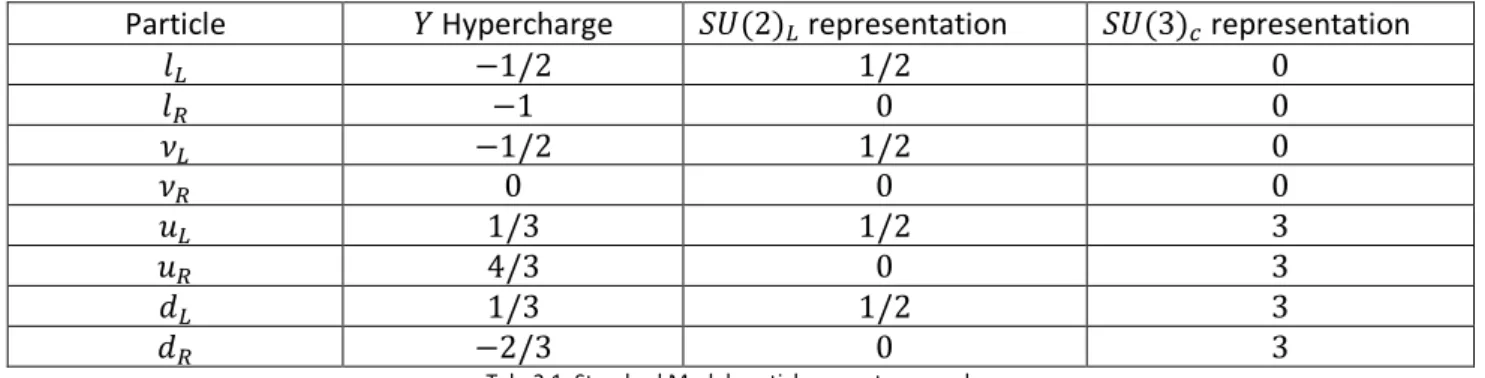
Particle classification assigns them the following quantum numbers:

Particle 𝑌 Hypercharge 𝑆𝑈(2)𝐿 representation 𝑆𝑈(3)𝑐 representation

𝑙𝐿 −1/2 1/2 0 𝑙𝑅 −1 0 0 𝜈𝐿 −1/2 1/2 0 𝜈𝑅 0 0 0 𝑢𝐿 1/3 1/2 3 𝑢𝑅 4/3 0 3 𝑑𝐿 1/3 1/2 3 𝑑𝑅 −2/3 0 3

Tab. 2.1. Standard Model particles quantum numbers

The Lagrangian written in the precedent form is clearly gauge-invariant, making various substitutions we obtain ℒ𝐹 _{= ℒ} 0 𝐹 _{+ ℒ} 𝐼 𝐹 _(2.1.33) ℒ0𝐹 = 𝑖 � ψ�𝐹𝛾𝜇𝜕𝜇ψ𝐹 𝐹𝑒𝑟𝑚𝑖𝑜𝑛𝑖 (2.1.34)

that is the free (quadratic) part, and ℒ𝐼𝐹 = 𝑞𝐹ψ�𝐹𝛾𝜇ψ𝐹𝐴𝜇− 𝑔 √2�ψ�𝐹−𝛾𝜇� 1 − 𝛾5 2 � ψ𝐹+𝑊𝜇+ ψ�𝐹+𝛾𝜇� 1 − 𝛾5 2 � ψ𝐹−𝑊𝜇+� − 𝑔 𝐶𝑜𝑠(𝜃𝑊) ψ�𝐹𝛾 𝜇_��𝑡 3,𝐹− 𝑞𝐹𝑆𝑖𝑛2(𝜃𝑊)� �1 − 𝛾_{2 � +}5 �−𝑞𝐹𝑆𝑖𝑛2(𝜃𝑊)� �1 + 𝛾_{2 �}5 � ψ𝐹𝑍𝜇 − 𝑔𝑆ψ�𝑄𝜆_{2 𝛾}𝑎 𝜇ψ𝑄𝐴𝑎,𝜇 (2.1.35)

that is the interaction part, where sum over 𝐹 (all the fermions), over the couples (𝐹+, 𝐹−) (couple of fermions belonging to the same 𝑆𝑈(2)𝐿 doublet respectively with 𝑡3= +1/2 and 𝑡3= −1/2) and over the

quarks 𝑄 is assumed.

From this term Feynman rules for the interaction vertices of fermion with gauge bosons can be obtained.

2.1.4 Higgs Field Lagrangian

ℒ𝐻 _{= [𝐷}𝜇_Φ]+_�𝐷

𝜇Φ� + 𝜇2‖Φ‖2− 𝜆‖Φ‖4 (2.1.36)

where the field Φ is a weak isospin doublet, it has Hypercharge 𝑌 = +1 and a non-zero vacuum expectation value: Φ� = 1 √2� 0 𝜇 √𝜆+ 𝜌�� 𝑒 −𝑖𝑔𝜃� 𝜎𝚤₂𝑖 _(2.1.37)

17

𝐷𝜇= 𝜕𝜇+ 𝑖𝑔𝑇𝑎𝑛(𝜃𝑊)𝑌𝐵𝜇+𝑖𝑔_{2 𝑊}𝑖,𝜇𝜎𝑖 (2.1.38)

The Lagrangian written in the precedent form is once again clearly gauge-invariant. Expanding we obtain various terms: ℒ𝐻 _{= ℒ} 0𝐻+ ℒ𝐼𝐻 (2.1.39) ℒ0𝐻 =1_{2 𝜕}𝜇𝜌𝜕𝜇𝜌 −1₂(2𝜇2)𝜌2+ �1_{2 𝑔} 𝜇 √𝜆� 𝑊𝜇+𝑊𝜇+ 1 2 � 1 2 𝑔 𝐶𝑜𝑠𝜃𝑊 𝜇 √𝜆� 𝑍𝜇𝑍𝜇 (2.1.40) In the free term we can identify two terms that give masses to the 𝑊 and 𝑍 bosons.

ℒ𝐼𝐻 =1_{2 𝑔}2 𝜇 √𝜆𝑊𝜇+𝑊𝜇𝜌 + 1 4 𝑔2𝑊𝜇+𝑊𝜇𝜌2+ 𝑔2 4𝐶𝑜𝑠2_(𝜃 𝑊) 𝜇 √𝜆𝑍𝜇𝑍𝜇𝜌 + 𝑔2 8𝐶𝑜𝑠2_(𝜃 𝑊) 𝑍𝜇𝑍 𝜇_𝜌2_{− √𝜆𝜇𝜌}3 −1 4 𝜆𝜌4 (2.1.41)

As usual from this term Feynman rules for the interaction vertices can be obtained.

2.1.5 Higgs’s and fermions’s couplings Lagrangian

ℒ𝐹𝐻 _{= −�Ψ�}

𝐿,𝑎𝑀𝐿,𝑎𝑏Ψ𝑅Φ + Φ+Ψ�𝑅,𝑎𝑀𝐿,𝑎𝑏+ Ψ𝐿� − �Ψ�𝐿,𝑎𝑀𝜈,𝑎𝑏Ψ𝑅Φ� + Φ�+Ψ�𝑅,𝑎𝑀𝜈,𝑎𝑏+ Ψ𝐿�

− �Ψ�𝑄,𝐿,𝑎𝑀𝑄𝑢,𝑎𝑏Ψ𝑄,𝑅Φ − Φ+Ψ�𝑄,𝑅,𝑎𝑀𝑄𝑢,𝑎𝑏+ Ψ𝑄,𝐿�

− �Ψ�𝑄,𝐿,𝑎𝑀𝑄𝑑,𝑎𝑏Ψ𝑄,𝑅Φ� − Φ�+Ψ�𝑄,𝑅,𝑎𝑀𝑄𝑑,𝑎𝑏+ Ψ𝑄,𝐿� (2.1.42)

where we have grouped also right handed fields in column vectors for sake of simplicity

Ψ𝑅 = � ψ𝑒,𝐿 ψ𝜇,𝐿 ψ𝜏,𝐿 � Ψ𝑄,𝑅 = � ψ𝑢,𝐿 ψ𝑐,𝐿 ψ𝑡,𝐿 � (2.1.43)

The field Φ� is defined as:

Φ� = −𝑖[Φ+_𝜎

2]𝑇 (2.1.44)

𝑀𝐿,𝑎𝑏 is the mass matrix for leptons, that, if we assume that neutrinos are massless, can be diagonalized as

follows:

�𝑚0𝑒 𝑚0𝜇 00

0 0 𝑚𝜏

� (2.1.45)

without changing the interaction terms with the 𝑊 boson. This mass matrix can be diagonalized also if neutrinos are not massless, but in that case the interaction with the 𝑊 boson changes, as indeed we will see it happen with quarks.

𝑀𝜈,𝑎𝑏 is the mass matrix for neutrinos, its form depends on the masses of the neutrinos, and the neutrino

mixing factors. For the rest of this work we will ignore neutrino.

Finally 𝑀𝑄𝑢,𝑎𝑏 and 𝑀𝑄𝑑,𝑎𝑏 are the mass matrices for quarks, and in the form in which the Lagrangian has

18

left and right handed fields, but in this way the interaction 𝑞𝑞′𝑊 (charged current) won’t be diagonal anymore, but will be mediated by the CKM matrix.

𝑉 = �𝑉𝑉𝑢𝑑𝑐𝑑 𝑉𝑉𝑢𝑠𝑐𝑠 𝑉𝑉𝑢𝑏𝑐𝑏

𝑉𝑡𝑑 𝑉𝑡𝑠 𝑉𝑡𝑏

� (2.1.46)

Using the basis where the mass matrices are diagonal (the one commonly used), we can rewrite the Lagrangian separating the free part from the interaction part

ℒ𝐹𝐻 _{= ℒ}

0𝐹𝐻+ ℒ𝐼𝐹𝐻 (2.1.47)

ℒ0𝐹𝐻 = −𝑚𝐹ψ�𝐹ψ𝐹 (2.1.48)

ℒ𝐼𝐹𝐻 = −√𝜆_{𝜇 𝑚}𝐹ψ�𝐹ψ𝐹𝜌 (2.1.49)

Quark vertices with 𝑊 will acquire a multiplicative factor 𝑉𝑖𝑗, moreover charged current processes may

occur also between quarks of different generations (as non diagonal 𝑉𝑖𝑗 are not null). These transitions will

be called prohibited because they cause a variation of strangeness 𝑆, or of charm 𝐶, or of bottomness 𝐵, or of topness 𝑇.

NOTE: Alternatively there are other ways of describing neutrinos and of generating their masses, for example neutrinos may be described by a Majorana spinor, with only the left-handed component. The various descriptions lead to different consequences, but beyond the purpose of this work, and because of this here the simplest description has been adopted, with the use of sterile neutrinos (as right-handed neutrinos would have all null quantum numbers, and wouldn’t interact either by strong interaction or by electroweak interaction).

2.2 Feynman Rules for the Standard Model

2.2.1 How to obtain Feynman Rules for the propagators

Finding the Feynman rules for propagators in a formally correct way is usually very complex, as there aren’t unique expressions, but they are gauge-dependent. Propagators depend on how we quantize the field, and this is also a crucial point to have a theory that is renormalizable at every renormalization order. The most correct way is the use of auxiliary fields called Ghost, with their propagators and interaction vertices. Those vertices won’t give any contribution at tree level, as ghosts are not physical particles, therefore this

procedure is not relevant for the purpose of this work. We will only list, in the next section, Feynman rules for propagators.

2.2.2 Feynman Rules for the propagators, Standard Model

Higgs Boson 𝐻

Higgs boson propagator

𝑖 𝑘2_{− 𝑚} 𝐻 2 Photon 𝛾 Photon propagator −𝑖𝑔_𝑘𝛼𝛽₂ 𝑊 Boson 𝑊 boson propagator 𝑖−𝑔𝛼𝛽+ 𝑘_𝛼𝑘_𝛽 𝑀𝑊2 𝑘2_{− 𝑀} 𝑊2

19 Fermion 𝐹 Fermion propagator 𝑖𝛾𝜇𝑝𝜇+ 𝑚𝐹 𝑝2_{− 𝑚} 𝐹 2 Gluon 𝑔 Gluon Propagator −𝑖𝑔_𝑘𝛼𝛽₂ 𝛿𝑎𝑏 𝑍 Boson 𝑍 boson propagator 𝑖−𝑔𝛼𝛽+ 𝑘𝛼𝑘𝛽 𝑀_𝑍2 𝑘2_{− 𝑀} 𝑍2 Tab 2.2 Feynman rules for propagators, Standard Model

2.2.3 How to obtain Feynman Rules for vertices

The action, at first order, is

𝑆 = −𝑖 � 𝑑4_𝑥ℋ

𝑖𝑛𝑡 = −𝑖 � 𝑑4𝑥(−ℒ𝐼) = 𝑖 � 𝑑4𝑥(ℒ𝐼) (2.2.1)

We can find Feynman rules for the vertex by making functional derivatives in relation to the fields of this term. For example

ℒ𝐼𝐹 = 𝑞𝐹ψ�𝐹𝛾𝜇ψ𝐹𝐴𝜇 (2.2.2) 𝑉(𝑝1, … , 𝑝𝑛) =_𝛿ψ�𝛿 𝐹 𝛿 𝛿ψ𝐹 𝛿 𝛿𝐴𝜇𝑆 = 𝑖 𝛿 𝛿ψ�𝐹 𝛿 𝛿ψ𝐹 𝛿 𝛿𝐴𝜇� 𝑑 4_𝑥𝑞 𝐹ψ�𝐹𝛾𝜇ψ𝐹𝐴𝜇 = 𝑖𝑞𝐹𝛾𝜇 (2.2.3)

2.2.4 Feynman Rules for vertices, Standard Model

Here follows a list of the rules, but only of those that are necessary to this work. 𝐹𝐹𝛾 Vertex Fermion-Fermion-Photon Vertex 𝑖𝑞𝛾𝜇 𝑄𝑄𝑔 Vertex Quark-Quark-Gluon Vertex 𝑖𝑔𝑆𝜆_{2 𝛾}𝑎 𝜇 𝑔𝑔𝑔 Vertex 3 Gluons Vertex 𝑔𝑆𝑓𝑎𝑏𝑐[𝑔𝜇𝜈(𝑘 − 𝑝)𝜌+ 𝑔𝜈𝜌(𝑘 − 𝑝)𝜇 + 𝑔𝜌𝜇_{(𝑘 − 𝑝)}𝜈_]

Ingoing momenta, gluon indices (𝜇, 𝑎); (𝜈, 𝑏); (𝜌, 𝑐)

Vertice 𝑔𝑔𝑔𝑔 4 Gluons Vertex −𝑖𝑔𝑆2[𝑓𝑎𝑏𝑒𝑓𝑐𝑑𝑒(𝑔𝜇𝜌𝑔𝜈𝜎− 𝑔𝜇𝜎𝑔𝜈𝜌) + 𝑓𝑎𝑐𝑒𝑓𝑏𝑑𝑒(𝑔𝜇𝜈𝑔𝜌𝜎− 𝑔𝜇𝜎𝑔𝜈𝜌) + 𝑓𝑎𝑑𝑒𝑓𝑏𝑐𝑒(𝑔𝜇𝜈𝑔𝜌𝜎− 𝑔𝜇𝜌𝑔𝜈𝜎)] Gluon indices (𝜇, 𝑎); (𝜈, 𝑏); (𝜌, 𝑐); (𝜎, 𝑑)

20

2.3 Running Coupling Constant

When one renormalizes the theory, one finds that coupling constants values are modified if compared to the bare ones appearing in the Lagrangian, these variations are due to diagrams such as:

Fig. 2.1. Feynman Diagrams contributing to the coupling constant renormalization

While these variations are negligible at tree level in electroweak interactions, in QCD it is not possible to neglect these corrections, in fact 𝛼𝑆 varies of orders of magnitude depending on the energy of the process:

at low energy, 𝛼𝑆 is very large and so partons are in the “infrared slavery”, that is they are confined;

instead, at high energy, partons are in the “ultraviolet freedom”, 𝛼𝑆 is very small and particles are

nearly-free. In other words, at low momenta subsequent orders of renormalization give a large contribution, while at high momenta their contributions are gradually suppressed.

The running coupling constant one loop equation is 𝑑

𝑑 𝐿𝑜𝑔 �𝑄_𝑀�𝑔𝑠 = 𝛽(𝑔𝑠) (2.3.1) where 𝛽 is, in the case of 𝑆𝑈(𝑁𝑐) symmetry with 𝑁𝑐 colors and 𝑛𝑓 flavors

𝛽(𝑔) = −_(4𝜋)𝑔𝑠3₂�11 3 𝑁𝑐− 2 3 𝑛𝑓� = − 𝑏0𝑔𝑠3 (4𝜋)2 (2.3.2)

Then in the case here examined

𝛽(𝑔) = −_(4𝜋)7𝑔𝑠3₂ (2.3.3) and one obtains

𝛼𝑠(𝑄) = 𝛼𝑠 1 + 7𝛼_{2𝜋 𝐿𝑜𝑔 �}𝑠 _𝑀�𝑄 = 1 1 𝛼𝑠+ 72𝜋 𝐿𝑜𝑔 � 𝑄 𝑀� (2.3.4)

21

2.4 Two body processes general Kinematics

2.4.1 Degrees of freedom

In a two body process, initial state is uniquely determined by the two four-momenta 𝑃1𝜇, 𝑃2𝜇, that is by 8

quantities.

These 8 quantities are constrained by the on-shell condition

𝑃₁𝜇𝑃1𝜇= 𝑚12, 𝑃2𝜇𝑃2𝜇= 𝑚22 (2.4.1)

therefore only 6 quantities are independent. Similarly, the final state is completely determined by 6 quantities.

Because of four-momenta conservation, these 6 quantities are related to the initial ones by a set of 4 equations, therefore the final state has only 2 degrees of freedom, that are the 𝜃 and 𝜑 angles in relation to the direction of the center of mass, that we will call 𝑐𝑜𝑚 from now on.

Of these 6 quantities, one may find out that:

4 quantities are the four momenta of the center of mass, the other 2 ones are a direction in space. Going back to the final state, as stated above, it has only 2 degrees of freedom, and then the cross section may be written in differential form in this way:

𝑑𝜎 = 𝑑𝜎

𝑑𝐶𝑜𝑠𝜃𝑑𝜑(𝐸𝑐𝑑𝑚, 𝜃, 𝜑)𝑑𝐶𝑜𝑠𝜃𝑑𝜑 (2.4.2)

In the center of mass frame, all processes have azimuthal symmetry, therefore we can remove the banal dependence on 𝜑 by integrating the above equation, obtaining as a result a multiplicative 2𝜋 factor.

2.4.2 Mandelstam variables

When working on two body processes it is useful to use Mandelstam variables, that are 3 variables that completely specify initial and final state in the center of mass frame. They are defined as follows:

Fig. 2.2. Two body process

𝑠 = (𝑝 + 𝑝′₎𝜇_{(𝑝 + 𝑝′)} 𝜇= (𝑘 + 𝑘′)𝜇(𝑘 + 𝑘′)𝜇 (2.4.3) 𝑡 = (𝑘 − 𝑝)𝜇_{(𝑘 − 𝑝)} 𝜇= (𝑝′− 𝑘′)𝜇(𝑝′− 𝑘′)𝜇 (2.4.4) 𝑢 = (𝑘′_{− 𝑝)}𝜇_(𝑝′_{− 𝑝)} 𝜇= (𝑝′− 𝑘)𝜇(𝑝′− 𝑘)𝜇 (2.4.5)

22

The only variables on which the cross section depends are 𝐸𝑐𝑑𝑚 and 𝜃, that are 2, consequently there must

be some relation between these 3 variables. The relation is

𝑠 + 𝑡 + 𝑢 = � 𝑚_𝑖2 4 𝑖=1

(2.4.6)

When 𝑚2_{≪ 𝑠 one can use the approximated relation}

𝑠 + 𝑡 + 𝑢 = 0 (2.4.7)

In this approximation the relations between Mandelstam variables and 𝐸𝑐𝑑𝑚 and 𝜃 variables are:

Fig. 2.3. Momenta in a two body process

𝑠 = (𝑝 + 𝑝′₎𝜇_{(𝑝 + 𝑝′)} 𝜇= 4𝐸𝑐𝑑𝑚2 (2.4.8) 𝑡 = (𝑘 − 𝑝)𝜇_{(𝑘 − 𝑝)} 𝜇= −4𝐸𝑐𝑑𝑚2 �1 − 𝐶𝑜𝑠𝜃₂ � = −𝑠 �1 − 𝐶𝑜𝑠𝜃₂ � (2.4.9) 𝑢 = (𝑘′_{− 𝑝)}𝜇_(𝑝′_{− 𝑝)} 𝜇= −4𝐸𝑐𝑑𝑚2 �1 + 𝐶𝑜𝑠𝜃₂ � = −𝑠 �1 + 𝐶𝑜𝑠𝜃₂ � (2.4.10) As 𝑑𝑡 =𝑠_{2 𝑑𝐶𝑜𝑠𝜃 (2.4.11)} we can write the differential cross section in the form

𝑑𝜎 =_{𝑑𝐶𝑜𝑠𝜃𝑑𝜑}𝑑𝜎 (𝐸𝑐𝑑𝑚, 𝜃)𝑑𝐶𝑜𝑠𝜃_{𝑑𝑡 𝑑𝑡𝑑𝜑 → 𝑑𝜎 =}𝑑𝜎_𝑑𝑡(𝑠, 𝑡)𝑑𝑡 (2.4.12) where 𝑑𝜎 𝑑𝑡(𝑠, 𝑡) = 𝑑𝜎 𝑑𝐶𝑜𝑠𝜃𝑑𝜑(𝐸𝑐𝑑𝑚(𝑠), 𝜃(𝑠, 𝑡)) 𝑠 2 2𝜋 = 𝜋𝑠 𝑑𝜎 𝑑𝐶𝑜𝑠𝜃𝑑𝜑(𝐸𝑐𝑑𝑚(𝑠), 𝜃(𝑠, 𝑡)) (2.4.13) All the cross sections will be written in this form, that is the most used in literature. Total cross section will be

𝜎(𝑠) = �𝑡𝑚𝑎𝑥𝑑𝑡𝑑𝜎_𝑑𝑡(𝑠, 𝑡)

𝑡𝑚𝑖𝑛

23

2.4.3 Channels for the processes

A two body process usually takes place through one of the following 3:

𝑠 channel: incident particles annihilate at a point 𝑥, a virtual boson propagates till a point 𝑦 where the two final particles are created

Fig. 2.4. Feynman diagram of an 𝑠 channel process

This channel contributes to the cross section with a term proportional to

𝜎𝑠 ∝𝑡 2_{+ 𝑢}2

𝑠2 (2.4.15)

𝑡 and 𝑢 channels: the two particles exchange a virtual boson, and scatter

Fig. 2.5. Feynman diagrams 𝑡 and 𝑢 channel processes

These channels contribute to the cross section with terms proportional, respectively, to

𝜎𝑡 ∝𝑢 2_{+ 𝑠}2 𝑡2 (2.4.16) 𝜎𝑢∝𝑠 2_{+ 𝑡}2 𝑢2 (2.4.17)

Every elementary process may occur using some, or all, these channels, depending on the particles involved.

For example 𝑞𝑞� → 𝑞′𝑞�′ may occur using only 𝑠 channel, because final particles are different from the initial ones and because of this they have to annihilate.

Instead 𝑞𝑞′ _{→ 𝑞𝑞′ may use only 𝑡 channel, it cannot use 𝑠 channel because two different quarks cannot}

24

2.5 Cross section calculation of elementary processes between partons

2.5.1 𝒈𝒈 → 𝒈𝒈

Feynman diagrams for this process are

Fig. 2.6. Feynmann diagrams for the Gluon Gluon to Gluon Gluon process

𝑑𝜎 𝑑𝑡(𝑔𝑔 → 𝑔𝑔) = 9𝜋𝛼𝑠2 2𝑠2 �3 − 𝑡𝑢 𝑠2− 𝑢𝑠 𝑡2 − 𝑠𝑡 𝑢2� (2.5.1)

This result must be divided by 2 because of the presence of identical particles in the final state.

*NOTE: while calculating, one must consider only the physical polarizations of gluons

2.5.2 𝒈𝒈 → 𝒒𝒒�

Feynman diagrams for this process are*

Fig. 2.7. Feynman diagrams for the Gluon Gluon to Quark Anti-Quark process

𝑑𝜎 𝑑𝑡(𝑔𝑔 → 𝑞𝑞�) = 𝜋𝛼𝑠2 6𝑠2� 𝑢 𝑡 + 𝑡 𝑢 − 9 4 𝑡2_{+ 𝑢}2 𝑠2 � (2.5.2)

*NOTE: while calculating, one must consider only the physical polarizations of gluons, ad adding the 𝑔ℎ𝑜𝑠𝑡 − 𝑎𝑛𝑡𝑖𝑔𝑜𝑠𝑡 → 𝑞𝑞� diagram

2.5.3 𝒒𝒒�

𝒈𝒈

The matrix element is the same as the one of the previous process, one must average on the quark colors instead of the gluon colors, and this contributes with a (8/3)2 _factor

𝑑𝜎 𝑑𝑡(𝑞𝑞� → 𝑔𝑔) = 32𝜋𝛼𝑠2 27𝑠2 � 𝑢 𝑡 + 𝑡 𝑢 − 9 4 𝑡2_{+ 𝑢}2 𝑠2 � (2.5.3)

25

2.5.4 𝒈𝒒 → 𝒈𝒒

It can be obtained by crossing from 𝑔𝑔 → 𝑞𝑞�, that is exchanging 𝑠 with 𝑡, and multiplying by an 8/3 factor because of the average on the initial states

𝑑𝜎 𝑑𝑡(𝑔𝑞 → 𝑔𝑞) = 4𝜋𝛼𝑠2 9𝑠2 �− 𝑢 𝑠 + 𝑠 𝑢 + 9 4 𝑠2_{+ 𝑢}2 𝑡2 � (2.5.4) NOTE: crossing must be done using the cross section without the 1 2� factor for identical particles.

2.5.5 𝒒𝒒� → 𝒒𝒒�

Feynman diagrams for this process are

Fig. 2.8. Feynman diagrams for the Quark Anti-Quark to Quark Anti-Quark (of the same flavour) process

𝑑𝜎 𝑑𝑡(𝑞𝑞� → 𝑞𝑞�) = 4𝜋𝛼𝑠2 9𝑠2 � 𝑢2_{+ 𝑠}2 𝑡2 + 𝑡2_{+ 𝑢}2 𝑠2 − 2 3 𝑢2 𝑠𝑡� (2.5.5)

2.5.6 𝒒𝒒 → 𝒒𝒒

It can be obtained by crossing from the previous process, that is exchanging 𝑠 with 𝑢 𝑑𝜎 𝑑𝑡(𝑞𝑞 → 𝑞𝑞) = 4𝜋𝛼𝑠2 9𝑠2 � 𝑠2_{+ 𝑢}2 𝑡2 + 𝑡2_{+ 𝑠}2 𝑢2 − 2 3 𝑠2 𝑢𝑡� (2.5.6)

This result must be divided by 2 because of the presence of identical particles in the final state.

2.5.7 𝒒𝒒� → 𝒒′𝒒�′

Feynman diagrams for this process are

Fig. 2.9. Feynman diagrams for the Quark Anti-Quark to Quark Anti-Quark (of different flavour) process

𝑑𝜎 𝑑𝑡(𝑞𝑞� → 𝑞′𝑞�′) = 4𝜋𝛼𝑠2 9𝑠2 � 𝑡2_{+ 𝑢}2 𝑠2 � (2.5.7)

2.5.8 𝒒𝒒′ → 𝒒𝒒′

It can be obtained by crossing from the previous process, that is exchanging 𝑠 with 𝑡 𝑑𝜎 𝑑𝑡(𝑞𝑞′ → 𝑞𝑞′) = 4𝜋𝛼𝑠2 9𝑠2 � 𝑠2_{+ 𝑢}2 𝑡2 � (2.5.8)

26

2.6 Deep Inelastic Scattering

2.6.1 Useful variables

So far, only processes between elementary particles have been considered. Before analyzing proton-proton processes, it is necessary to know how the first ones (partons) are related to the second ones (protons). To do this, one may probe protons with deep inelastic scattering, that is scattering of high energy light particles.

In these processes, occurring at high energies, one may assume that only one quark interacts, exchanging a virtual photon.

Fig. 2.10. Deep Inelastic Scattering 𝑒𝑝 → 𝑒𝑋

The cross section for this process is 𝑑𝜎 𝑑𝑡 = 2𝜋𝑄_𝑖2_𝛼2 𝑠2 � 𝑠2_{+ 𝑢}2 𝑡2 � (2.6.1)

Let’s assume that the quark carries a fraction 𝑥 of the proton’s momenta, then, calling 𝑝 the quark’s momenta and 𝑃 the proton’s momenta, 𝑝 = 𝑥𝑃 and

𝑠 = (𝑝 + 𝑘)2 _{= 2𝑝𝑘 = 2𝑥𝑃𝑘 = 𝑥𝑠}′ _(2.6.2)

Let’s call 𝑞 the exchanged momenta; as the scattered quark is massless in our approximations, 0 = (𝑝 + 𝑞)2_{= 2𝑥𝑃𝑞 + 𝑞}2_{= 2𝑥𝑀𝜈 − 𝑄}2 _(2.6.3)

where new variables have been defined

𝑄2 _{= −𝑞}2_{= −𝑡 (2.6.4)}

𝜈 =𝑃𝑞_{𝑀 =2𝑀𝑥 (2.6.5)}𝑄2 that are useful variables as they can be experimentally observed.

Moreover, one must take into account that the probability that the quark carries a fraction 𝑥 of the proton’s momenta will be given by a distribution function depending on 𝑄2 _{and 𝜈, that is called 𝐹}

1(𝑄2, 𝜈),

and that the probability that a parton has a fraction of the proton’s momenta between 𝑥 =_2𝑀𝜈𝑄2 and 𝑥 + 𝑑𝑥 will be equal to 𝐹1(𝑄2, 𝜈)𝑑𝑥.

27 𝑑𝜎 𝑑𝑥𝑑𝑄2 = 2𝜋𝑄𝑖2𝛼2 𝑄4 �1 + �1 − 𝑄2 𝑥𝑠� 2 � 𝐹1(𝑄2, 𝜈) (2.6.6)

2.6.2 Bjorken’s Scaling

Bjorken’s scaling hypothesis is that in the limit

�𝑄 → ∞𝜈 → ∞

𝑥 < ∞ (2.6.7) 𝐹1(𝑄2, 𝜈) → 𝑓(𝑥) (2.6.8)

In reality, this isn’t true experimentally, more precisely

𝐹1(𝑄2, 𝜈) → 𝑓(𝑥, 𝑄) (2.6.9)

where the 𝑄 is very weak.

The meaning of Bjorken’s scaling is that at high energies strong interactions between quarks are negligible, that is quarks are free. The running coupling constant goes to zero at high energies, but only logaritmically, because of this the 𝑄 dependence vanishes very slowly.

2.7 Parton Distribution Functions

Inside protons, gluons and quarks may be found, with some probability distribution that depends on the fraction of the total momenta of the proton carried by the parton.

These functions, called PDF, Parton Distribution Functions, can be obtained from Deep Inelastic Scattering experimental results of neutrinos and electros on protons.

Fig. 2.11. Plot of the functions 𝑥𝑓(𝑥) used in MonteCarlo simulations, black line for Gluons, green/orange lines for 𝑢𝑢�, red/blue lines for 𝑑𝑑̅, purple line for the couples 𝑠𝑠̅ and brown for the couples 𝑐𝑐̅. Distributions at 𝑄 = 2𝐺𝑒𝑉

28

As one may see from the plot, there is a quark, antiquark and gluons mix. Proton is a bound state 𝑢𝑢𝑑, but it contains also other quarks and antiquarks. Anyway there must be an excess of two 𝑢 quarks and one 𝑑 quark, so that the following relations must hold

� 𝑑𝑥[𝑓𝑢(𝑥) − 𝑓𝑢�(𝑥)] 1

0 = 2 � 𝑑𝑥[𝑓𝑑(𝑥) − 𝑓𝑑�(𝑥)] 1

0 = 1 (2.7.1)

Instead, as for the other quarks and antiquarks, the following relation applies 𝑓𝑞(𝑥) = 𝑓𝑞�(𝑥) (2.7.2)

NOTE: in the case 𝑞 = 𝑠 there might be a small asymmetry that violates this relation.

Finally, the sum of the momenta of the various constituents must be equal to the proton’s momenta, therefore � 𝑑𝑥 𝑥 �𝑓𝑔(𝑥) + � �𝑓𝑞(𝑥) + 𝑓𝑞�(𝑥)� 𝑞 � 1 0 = 1 (2.7.3)

Experimentally one may observe that proton is dominated by gluons

� 𝑑𝑥 𝑓𝑔(𝑥) 1

0 > 30 (2.7.4)

In the appendix (section 7.2) PDF plots obtained from H1, ZEUS HERA I and II data’s have been reported.

2.8 Proton-Proton processes

Now we want to compute the cross section for a proton-proton process, like the one in the picture:

Fig. 2.12. Hard 𝑝𝑝 → 𝐽𝐽 scattering

The contribution to the cross section of the elementary process 1 + 2 → 3 + 4 for what has been said so far is

𝑓1(𝑥1)𝑓2(𝑥2)𝑑𝜎_𝑑𝑡(1 + 2 → 3 + 4) (2.8.1)

Particles 1 and 2 may be one of all the proton’s constituents, therefore to calculate the total cross section it is necessary to sum this contribution over all the possible initial partons

29 𝑑𝜎 𝑑𝑥1𝑑𝑥2𝑑𝑡(𝑝𝑝 → 3 + 4) = � 𝑓1(𝑥1)𝑓2(𝑥2) 𝑑𝜎 𝑑𝑡(1 + 2 → 3 + 4) 1,2 (2.8.2)

The total inclusive (sum over possible 3 and 4 particles) cross section will be then

𝜎 = � � 𝑑𝑥1𝑑𝑥2𝑑𝑡𝑓1(𝑥1)𝑓2(𝑥2)𝑑𝜎_𝑑𝑡(1 + 2 → 3 + 4) 𝐷

1,2,3,4

(2.8.3)

30

3 Gravity Interactions

3.1 Einstein’s Equation

Einstein’s equation of General relativity is

𝑅𝜇𝜈 −1_{2 𝑅𝑔}𝜇𝜈 =8𝜋𝐺_𝑐4 𝑇𝜇𝜈 (3.1.1)

Adding the Extra-Dimensions then the equation will have 𝐷 = 4 + 𝛿 dimensions:

𝑅𝑎𝑏−1_{2 𝑅𝑔}𝑎𝑏= −(2𝜋) 𝛿

𝑀_𝐷2+𝛿𝑇𝑎𝑏 (3.1.2)

In general the presence of the four dimensional mainfold, of the world where we live, will produce a non-flat 𝐷-dimensional metric. Anyway at distances larger than _𝑀1

𝐷 it is reasonable that metric will be essentially

flat. For this reason while studying the emission of soft gravitons with a transverse momenta much smaller than 𝑀𝐷, and therefore distances much larger than _𝑀1

𝐷, one may expand the metric about the

Minkowskian one

𝑔𝑎𝑏 = 𝜂𝑎𝑏+2(2𝜋) 𝛿 2⁄

𝑀_𝐷1+𝛿 2⁄ ℎ𝑎𝑏 (3.1.3)

Substituting and linearizing the equation, that is retaining only the linear terms of ℎ𝑎𝑏, one obtains

𝜕2_ℎ

𝑎𝑏− 𝜕𝑎𝜕𝑐ℎ𝑐𝑏− 𝜕𝑏𝜕𝑐ℎ𝑐𝑎+ 𝜕𝑎𝜕𝑏ℎ𝑐𝑐− 𝜂𝑎𝑏𝜕2ℎ𝑐𝑐+ 𝜂𝑎𝑏𝜕𝑐𝜕𝑑ℎ𝑐𝑑= −(2𝜋) 𝛿 2⁄

𝑀_𝐷1+𝛿 2⁄ 𝑇𝑎𝑏 (3.1.4)

3.1.1 Kaluza-Klein modes

One can assume now, for simplicity, that the extra dimensions have the topology of a torus, and cyclical bounds are imposed on this coordinates

𝑥𝑎 _{= �𝑥}𝜇_{, 𝑦}1_{… 𝑦}𝛿_{� (3.1.5)}

𝑦𝑖 _{→ 𝑦}𝑖_{+ 2𝜋𝑅 (3.1.6)}

Expanding ℎ𝑎𝑏 in Fourier series

ℎ𝑎𝑏(𝑥𝑎) =_(2𝜋𝑅)1 _{𝛿 2}⁄ � ℎ𝑎𝑏𝑛 (𝑥𝜇)𝑒𝑖 𝑛𝑗_𝑦𝑗 𝑅 ∞ 𝑛𝑖=−∞ (3.1.7)

ℎ𝑎𝑏𝑛 (𝑥𝜇) are called Kaluza-Klein modes, they live in the usual space-time.

As ordinary matter is confined to the four dimensional mainfold of our universe, it is possible to write 𝑇𝑎𝑏(𝑥𝑎) = 𝜂𝑎𝜇𝜂𝑏𝜈𝑇𝜇𝜈(𝑥𝜇)𝛿(𝑦) (3.1.8)

31

The singularity of the delta function and the fact that our universe is confined to a four dimensional

mainfold are only approximations, as both of them must have a finite thickness. Anyway this approximation is important only at short distances, while it is negligible at large distances, as happens in our case. For our goals, we only need to know that 𝐾𝐾 modes of 𝑇𝑎𝑏 are independent of 𝑛 for small 𝑛, that is 𝑛 ≪ 𝑀𝐷𝑅.

This means that all 𝐾𝐾 modes have the same coupling to the ordinary matter, and allows us make accurate predictions on the cross sections.

3.1.2 Physical Fields and Gauge-dependent Fields

The following is from reference [3]. Substituting the expression for the Fourier transform of ℎ𝑎𝑏 in

Einstein’s equation, and integrating over the coordinates of the extra dimensions, one obtains the following equations: (𝜕2_{+ 𝑛�}2_)ℎ 𝜇ν(𝑛)− �𝜕𝜇𝜕𝜆ℎ𝜈(𝑛)𝜆+ 𝑖𝑛�𝑗𝜕𝜇ℎ(𝑛)𝑗𝜈 + 𝜕𝜈𝜕𝜆ℎ𝜇(𝑛)𝜆+ 𝑖𝑛�𝑗𝜕𝜈ℎ𝜇(𝑛)𝑗� + �𝜕𝜇𝜕𝜈− 𝜂𝜇𝜈(𝜕2+ 𝑛�2)� �ℎ𝜆(𝑛)𝜆+ ℎ𝑗(𝑛)𝑗� + 𝜂𝜇𝜈�𝜕𝜆𝜕𝜎ℎ𝜆𝜎(𝑛)+ 2𝑖𝑛�𝑗𝜕𝜆ℎ𝜆(𝑛)𝑗− 𝑛�𝑗𝑛�𝑘ℎ𝑗𝑘(𝑛)� = − (8𝜋)1 2⁄ 𝑅𝛿 2⁄ _𝑀 𝐷1+𝛿 2⁄ 𝑇𝜇𝜈 (3.1.9) (𝜕2_{+ 𝑛�}2_)ℎ 𝜇j(𝑛)− 𝜕𝜇𝜕𝜈ℎ𝑗(𝑛)𝜈− 𝑖𝑛�𝑘𝜕𝜇ℎ𝑗(𝑛)𝑘− 𝑖𝑛�𝑗𝜕𝜈ℎ𝜇(𝑛)𝜈+ 𝑛�𝑗𝑛�𝑘ℎ𝜇(𝑛)𝑘+ 𝑖𝑛�𝑗𝜕𝜇�ℎ𝜈(𝑛)𝜈+ ℎ𝑘(𝑛)𝑘� = 0 (3.1.10) (𝜕2_{+ 𝑛�}2_)ℎ 𝑗𝑘(𝑛)− �𝑖𝑛�𝑗𝜕𝜇ℎ𝑘(𝑛)𝜇− 𝑛�𝑗𝑛�𝑙ℎ(𝑛)𝑙𝑘 + 𝑖𝑛�𝑘𝜕𝜇ℎ𝑗(𝑛)𝜇− 𝑛�𝑘𝑛�𝑙ℎ𝑗(𝑛)𝑙� − �𝑛�𝑗𝑛�𝑘+ 𝜂𝑗𝑘(𝜕2+ 𝑛�2)� �ℎ𝜇(𝑛)𝜇+ ℎ𝑙(𝑛)𝑙� + 𝜂𝑗𝑘�𝜕𝜇𝜕𝜈ℎ𝜇𝜈(𝑛)+ 2𝑖𝑛�𝑙𝜕𝜇ℎ𝜇(𝑛)𝑙− 𝑛�𝑙𝑛�𝑚ℎ𝑙𝑚(𝑛)� = 0 (3.1.11)

where 𝜕2 _{operates only in the usual 4 dimensions, and it has been defined 𝑛�}

𝑗 =𝑛_𝑅𝑗 and 𝑛�2 = 𝑛�𝑗𝑛�𝑗.

Furthermore 𝜂𝜇𝜈 = (+, −, −, −) and 𝜂𝑗𝑘= −𝛿𝑗𝑘.

To solve this system it is better to rewrite it in terms of the following dynamic variables:

𝐺𝜇𝜈(𝑛)= ℎ𝜇ν(𝑛)+𝜅_{3 �𝜂}𝜇𝜈+𝜕𝜇_𝑛�𝜕₂𝜈� 𝐻(𝑛)− 𝜕𝜇𝜕𝜈𝑃(𝑛)+ 𝜕𝜇𝑄𝜈(𝑛)+ 𝜕𝜈𝑄𝜇(𝑛) (3.1.12) 𝑉_𝜇𝑗(𝑛)= 1 √2�𝑖ℎ𝜇j (𝑛)_{− 𝜕} 𝜇𝑃𝑗(𝑛)− 𝑛�𝑗𝑄𝜇(𝑛)� (3.1.13) 𝑆_𝑗𝑘(𝑛)= ℎ_𝑗𝑘(𝑛)−_{𝛿 − 1 �𝜂}𝜅 𝑗𝑘+𝑛�_𝑛�𝑗𝑛�2𝑘� 𝐻(𝑛)+ 𝑛�𝑗𝑃𝑘(𝑛)+ 𝑛�𝑘𝑃𝑗(𝑛)− 𝑛�𝑗𝑛�𝑘𝑃(𝑛) (3.1.14) 𝐻(𝑛)₌1 𝜅�ℎ𝑗(𝑛)𝑗+ 𝑛�2𝑃(𝑛)� (3.1.15) 𝑄𝜇(𝑛)= −𝑖_𝑛�𝑛�𝑗2ℎ𝜇(𝑛)𝑗 (3.1.16) 𝑃_𝑗(𝑛)=𝑛�_𝑛�𝑘₂ℎ_𝑗(𝑛)𝑘+ 𝑛�𝑗𝑃(𝑛) (3.1.17) 𝑃(𝑛)=𝑛�𝑗_𝑛�𝑛�₄𝑘ℎ_𝑗𝑘(𝑛) (3.1.18)

32 where we have defined the factor

𝜅 = �3(𝛿 − 1)_{𝛿 + 2 (3.1.19)}

Let’s check that the number of degrees of freedom is unchanged. The initial tensor is symmetric (4 + 𝛿) × (4 + 𝛿) tensor, therefore has (4+𝛿)(5+𝛿)₂ 𝑑. 𝑜. 𝑓.

𝐺𝜇𝜈(𝑛) is symmetric and therefore has 5 ∙4₂= 10 𝑑. 𝑜. 𝑓.,

𝑉_𝜇𝑗(𝑛) has 4 × 𝛿 components with the constrain 𝑛�𝑗_𝑉

𝜇𝑗(𝑛)= 0 and then has 4𝛿 − 4 = 4(𝛿 − 1)𝑑. 𝑜. 𝑓.

𝑆_𝑗𝑘(𝑛) is symmetric with null trace and the constrain 𝑛�𝑗_𝑆

𝑗𝑘(𝑛)= 0, then it has 𝛿(𝛿+1)

2 − 𝛿 − 1 =

(𝛿−2)(𝛿+1)

2 𝑑. 𝑜. 𝑓.

𝐻(𝑛) _{and 𝑃}(𝑛) _{are scalars and have then 1 𝑑. 𝑜. 𝑓. each,}

𝑄_𝜇(𝑛) has 4 𝑑. 𝑜. 𝑓.,

𝑃_𝑗(𝑛) has the constrain 𝑛�𝑗_𝑃

𝑗(𝑛)= 0 and therefore has 𝛿 − 1 𝑑. 𝑜. 𝑓.

The total is 10 +9₂𝛿 +1₂𝛿2₌(4+𝛿)(5+𝛿)

2 𝑑. 𝑜. 𝑓., the same as the ones of the initial tensor.

We may note that in the case 𝛿 = 1 the parametrization is singular because the fields 𝐻(𝑛)_{, 𝑃}(𝑛) _{and 𝑃} 𝑗(𝑛)

are no more independent. Anyway we are interested in the case 𝛿 > 1.

Contracting the indices of the previous equation with the metric, we find the following constrains on the fields: 𝜕𝜇_𝐺 𝜇ν(𝑛)= 1 𝑅𝛿 2⁄ _𝑀 𝐷1+𝛿 2⁄ 𝜕𝜈𝑇𝜆𝜆 3𝑛�2 (3.1.20) 𝐺_𝜇(𝑛)𝜇= 1 𝑅𝛿 2⁄ _𝑀 𝐷1+𝛿 2⁄ 𝑇_𝜇𝜇 3𝑛�2 (3.1.21) 𝜕𝜇_𝑉 𝜇j(𝑛) = 0 (3.1.22)

If we use these constrains in the equations 3.1.9 − 11, we obtain the following uncoupled equations:

(𝜕2_{+ 𝑛�}2_)𝐺 𝜇ν(𝑛)= 1 𝑅𝛿 2⁄ _𝑀 𝐷1+𝛿 2⁄ �−𝑇𝜇𝜈 + �𝜂𝜇𝜈 +𝜕𝜇_𝑛�𝜕₂𝜈�𝑇𝜆 𝜆 3 � (3.1.23) (𝜕2_{+ 𝑛�}2_)𝑉 𝜇j(𝑛)= 0 (3.1.24) (𝜕2_{+ 𝑛�}2_)𝑆 𝑗𝑘(𝑛)= 0 (3.1.25)

33 (𝜕2_{+ 𝑛�}2_)𝐻(𝑛)₌𝜅 3 1 𝑅𝛿 2⁄ _𝑀 𝐷1+𝛿 2⁄ 𝑇𝜇𝜇 (3.1.26)

These equations mean that only 𝐺𝜇𝜈(𝑛), 𝑉𝜇𝑗(𝑛), 𝑆𝑗𝑘(𝑛) and 𝐻(𝑛) are propagating particles, while 𝑄𝜇(𝑛), 𝑃(𝑛) and

𝑃_𝑗(𝑛) do not appear in the equations of motion. These fields are gauge-dependent, and therefore do not describe physical particles. To be more precise they can be all set to zero in every space-time point with an appropriate gauge transformation for each 𝑛 ≠. This gauge is called the Unitary Gauge.

3.1.3 Identification of the Particles

The equations for the field 𝐺𝜇𝜈(𝑛), in the vacuum, are:

(𝜕2_{+ 𝑛�}2_)𝐺

𝜇ν(𝑛)= 0 (3.1.27)

𝜕𝜇_𝐺

𝜇𝜈(𝑛)= 0 (3.1.28)

𝐺𝜇(𝑛)𝜇= 0 (3.1.29)

The first equation tells us that this field represents propagating bosons of mass 𝑛�2_{, while the second and}

the third ones cancel 5 of the 10 components, leaving only 5 non-zero components, corresponding to 5 particles of spin 2. Therefore this field describes 5 gravitons of mass 𝑛�2_{, that is the 𝑛-th 𝐾𝐾 eccitation.}

The field 𝑉_𝜇𝑗(𝑛) describes 𝛿 − 1 spin 1 particles, each with 3 degrees of freedom because of constrain 3.1.22. Anyway in the weak field approximation they do not couple with the energy-momentum tensor, so,

because of this, they are not relevant for this work.

For 𝛿 ≥ 2 there are (𝛿−2)(𝛿+1)₂ massive scalar particles described by the tensor 𝑆_𝑗𝑘(𝑛), anyway also these particles do not couple with the energy-momentum tensor, and then are not relevant for this work. Finally, there is the scalar particle 𝐻(𝑛) _{that couples only with the trace of the energy-momentum tensor.}

This trace is null for a conformally flat theory, therefore also this particle is negligible at tree level in processes with massless particles, in fact it can couple at tree level only proportionally to the masses of the particles, because of this its coupling is at best of order �𝑀𝑍

𝑀_𝐷� 2

~ �𝑀𝑍

𝑀_𝐸𝑊� 2

and can be then neglected.

Let’s compare the initial number of 𝑑. 𝑜. 𝑓. with the number of particles found, that is (𝛿+4)(𝛿+1)₂ . The difference between these two numbers is 2(𝛿 + 4). These degrees of freedom are associated with the gauge invariance.

To choose a gauge, first of all it is necessary to choose a constrain like the one of the harmonic gauge 𝜕𝑎ℎ𝑏𝑎=1_{2 𝜕}𝑏ℎ𝑎𝑎 (3.1.30)

that cancels 𝛿 + 4 degrees of freedom. Then, one may see that, like in QED, for a massless graviton there are still some degrees of freedom because of the freedom in the choice of the polarization, that can be canceled by demanding 𝜕2_𝜖

𝑎= 0, constrain that cancels 𝛿 + 4 degrees of freedom, for a total of

34

3.2 Gravitational Lagrangian

Starting from the 4 + 𝛿 dimensional Lagrangian density corresponding to Einstein’s equation 3.1.2

ℒ = −1_{2 ℎ}𝑎𝑏_𝜕2_ℎ

𝑎𝑏+1_{2 ℎ}𝑎𝑎𝜕2ℎ𝑏𝑏− ℎ𝑎𝑏𝜕𝑎𝜕𝑏ℎ𝑐𝑐+ ℎ𝑎𝑏𝜕𝑎𝜕𝑐ℎ𝑏𝑐 −(2𝜋) 𝛿 2⁄

𝑀_𝐷1+𝛿 2⁄ ℎ𝑎𝑏𝑇𝑎𝑏 (3.2.1) let’s follow the procedure of the previous sections, that is substituting the Fourier series and the fields parametrization, and considering the Unitary gauge. We obtain:

ℒ = � �−1_{2 𝐺}(−𝑛�⃗)𝜇ν_(𝜕2_{+ 𝑛�}2_)𝐺 𝜇ν(𝑛�⃗)+1_{2 𝐺}𝜇(−𝑛�⃗)𝜇(𝜕2+ 𝑛�2)𝐺ν(𝑛�⃗)ν− 𝐺(−𝑛�⃗)𝜇ν𝜕𝜇𝜕𝜈𝐺λ(𝑛�⃗)λ+ 𝐺(−𝑛�⃗)𝜇ν𝜕𝜇𝜕𝜆𝐺ν(𝑛�⃗)λ� 𝑛�⃗ + � �−1₄�𝜕𝜇𝑉𝜈𝑗(𝑛�⃗)− 𝜕𝜈𝑉𝜇𝑗(𝑛�⃗)� 2 +1_{2 𝑛�}2_𝑉(−𝑛�⃗)𝜇j_𝑉 𝜇𝑗(𝑛�⃗)−1_{2 𝑆}(−𝑛�⃗)𝑗𝑘(𝜕2+ 𝑛�2)𝑆𝑗𝑘(𝑛�⃗)−1_{2 𝐻}(−𝑛�⃗)(𝜕2+ 𝑛�2) 𝐻(𝑛�⃗)� 𝑛�⃗ + � �− 1 𝑅𝛿 2⁄ _𝑀 𝐷1+𝛿 2⁄ �𝐺(𝑛�⃗)𝜇ν₋𝜅 3 𝜂𝜇𝜈𝐻(𝑛�⃗)� 𝑇𝜇𝜈� 𝑛�⃗ (3.2.2) In QED 𝑇𝜇𝜈 =_{4 ψ}𝑖 ��𝛾𝜇𝜕𝜈+ 𝛾𝜈𝜕𝜇�ψ −₄𝑖�𝜕𝜈ψ�𝛾𝜇+ 𝜕𝜇ψ�𝛾𝜈�ψ +1_{2 𝑞ψ}��𝛾𝜇𝐴𝜈+ 𝛾𝜈𝐴𝜇�ψ + 𝐹𝜇λ𝐹𝜈𝜆 +1 4 𝜂𝜇𝜈𝐹𝜆𝜌𝐹𝜆𝜌 (3.2.3) One may notice that the trace of this tensor is zero. For the QCD the formula is similar, with the substitutions

𝑞𝐴𝜇→ 𝑔𝑠𝐴𝑎,𝜇𝜆 𝑎

2 , 𝐹𝜇𝜈 → 𝐹𝑆𝜇𝜈 (3.2.4)

3.3 Feynman rules

As for the Standard Model, one may calculate Feynman rules for vertices and propagators. Here is a list one the ones necessary for this work.

3.3.1 Feynman Rules for propagators

Feynman diagram for the graviton propagator

𝑖_𝑘2𝑃𝜇𝜈𝜌𝜎_{− 𝑚2} (3.3.1) where 𝑚2_{= 𝑛�}2 _{is the mass of the 𝑛-th 𝐾𝐾 mode and}

35 𝑃𝜇𝜈𝜌𝜎 =1₂�𝜂𝜇𝛼𝜂𝜈𝛽− 𝜂𝜇𝛽𝜂𝜈𝛼− 𝜂𝜇𝜈𝜂𝛼𝛽� −_2𝑚1₂�𝜂𝜇𝛼𝑘𝜈𝑘𝛽+ 𝜂𝜈𝛽𝑘𝜇𝑘𝛼+ 𝜂𝜇𝛽𝑘𝜈𝑘𝛼+ 𝜂𝜈𝛼𝑘𝜇𝑘𝛽� +1 6 �𝜂𝜇𝜈+ 2 𝑚2𝑘𝜇𝑘𝜈� �𝜂𝛼𝛽+ 2 𝑚2𝑘𝛼𝑘𝛽� (3.3.2)

The propagator of the massless propagator in 4 + 𝛿 dimensions instead is

𝑖𝑃𝜇𝜈𝜌𝜎

(0)

𝑘2 (3.3.3)

𝑃𝜇𝜈𝜌𝜎(0) =1₂(𝜂𝑎𝑐𝜂𝑏𝑑+ 𝜂𝑎𝑑𝜂𝑏𝑐) −_{𝛿 + 2 𝜂}1 𝑎𝑏𝜂𝑐𝑑+𝜀 − 1_2𝑘2 (𝜂𝑎𝑐𝑘𝑏𝑘𝑑+ 𝜂𝑏𝑑𝑘𝑎𝑘𝑐+ 𝜂𝑎𝑑𝑘𝑏𝑘𝑐+ 𝜂𝑏𝑐𝑘𝑎𝑘𝑑)(3.3.4)

where 𝜀 is the gauge-fixing parameter.

3.3.2 Feynman Rules for vertices

𝐹𝐹𝐺 vertex

Feynman diagram for the Fermion-Fermion-Graviton vertex −𝑖 (2𝜋)𝛿 2⁄ 𝑅𝛿 2⁄ _𝑀 𝐷1+𝛿 2⁄ 𝑊𝜇𝜈𝐹 𝛾𝛾𝐺 vertex

Feynman diagram for the Photon-Photon-Graviton vertex −𝑖 (2𝜋)𝛿 2⁄ 𝑅𝛿 2⁄ _𝑀 𝐷1+𝛿 2⁄ 𝑊_{𝜇𝜈𝛼𝛽}𝛾 𝑓𝑓𝛾𝐺 vertex

Feynman diagram for the Fermion-Fermion-Photon-Graviton vertex −𝑖𝑞 (2𝜋)𝛿 2⁄ 2𝑅𝛿 2⁄ _𝑀 𝐷1+𝛿 2⁄ 𝑋𝜇𝜈𝛼 𝑔𝑔𝑔𝐺 vertex

Feynman diagram for the Gluon-Gluon-Gluon-Graviton vertex 𝑔𝑠 (2𝜋) 𝛿 2⁄ 2𝑅𝛿 2⁄ _𝑀 𝐷1+𝛿 2⁄ 𝑓𝑎𝑏𝑐_𝑌 𝜇𝜈𝛼𝛽𝛾 𝑔𝑔𝐺 vertex

Feynman diagram for the Gluon-Gluon-Graviton vertex −𝑖 (2𝜋)𝛿 2⁄ 𝑅𝛿 2⁄ _𝑀 𝐷1+𝛿 2⁄ 𝛿𝑎𝑏𝑊𝜇𝜈𝛼𝛽𝛾 𝐹𝐹𝑔𝐺 vertex

Feynman diagram for the Fermion-Fermion-Gluon-Graviton vertex −𝑖𝑔𝑠 (2𝜋) 𝛿 2⁄ 2𝑅𝛿 2⁄ _𝑀 𝐷1+𝛿 2⁄ 𝜆12𝑎 2 𝑋𝜇𝜈𝛼

Tab. 3.1. Feynman rules for vertices, ADD model

Indices 𝜇, 𝜈 refer to the graviton. Indices 𝛼, 𝛽, 𝛾 refer, in order, to particles 1,2,3, if present. The same holds for color indices 𝑎, 𝑏, 𝑐.

𝑊𝜇𝜈𝐹 = (𝑘1+ 𝑘2)𝜇𝛾𝜈+ (𝑘1+ 𝑘2)𝜈𝛾𝜇 (3.3.5)

𝑊_{𝜇𝜈𝛼𝛽}𝛾 =1_{2 𝜂}𝜇𝜈�𝑘1𝛽𝑘2𝛼− (𝑘1𝜆𝑘2𝜆)𝜂𝛼𝛽� + 𝜂𝛼𝛽𝑘1𝜇𝑘2𝜈+ 𝜂𝜇𝛼��𝑘1𝜆𝑘2𝜆�𝜂𝜈𝛽− 𝑘1𝛽𝑘2𝜈� − 𝜂𝜇𝛽𝑘1𝜈𝑘2𝛼

+𝜇 ↔ 𝜈 (3.3.6) 𝑋𝜇𝜈𝛼 = 𝛾𝜇𝜂𝜈𝛼+ 𝛾𝜈𝜂𝜇𝛼

36

𝑌𝜇𝜈𝛼𝛽𝛾 = �𝑍𝜇𝜈𝛼𝛽𝛾(𝑘1) + 𝑍𝜇𝜈𝛼𝛽𝛾(𝑘2) + 𝑍𝜇𝜈𝛼𝛽𝛾(𝑘3)� + 𝜇 ↔ 𝜈 (3.3.7)

𝑍𝜇𝜈𝛼𝛽𝛾(𝑘1) = 𝑘1𝜇�𝜂𝜈𝛽𝜂𝛼𝛾− 𝜂𝜈𝛾𝜂𝛼𝛽� + 𝑘1𝛽�𝜂𝜇𝛼𝜂𝜈𝛾−1_{2 𝜂}𝜇𝜈𝜂𝛼𝛾� − 𝑘1𝛾�𝜂𝜇𝛼𝜂𝜈𝛽−1_{2 𝜂}𝜇𝜈𝜂𝛼𝛽� (3.3.8)

3.4 Real Graviton Production

3.4.1 Modes density

Now we can consider some processes whose theoretical results are relevant to be compared to collider’s experimental data, starting from real graviton production. 𝐾𝐾 excitations have masses 𝑛_𝑅 and therefore their masses are separated by a mass splitting factor of

∆𝑚~_{𝑅 = �}1 8𝜋𝑀𝐷2+𝛿 𝑀𝑃2 � 1/𝛿 = 𝑀𝐷�√8𝜋𝑀_𝑀 𝐷 𝑃 � 2/𝛿 ~ �_{𝑇𝑒𝑉�}𝑀𝐷 𝛿+2 2 ∙ 1012𝛿−31𝛿 _{𝑒𝑉 (3.4.1)}

If 𝛿 is not too big mass splitting is very small and one can consider it continuum: the number of modes between 𝑛 and 𝑛 + 𝑑𝑛 is 𝑑𝑁 = 2𝜋𝛿/2 Γ(𝛿/2) 𝑛𝛿−1𝑑𝑛 = 2𝜋𝛿/2 Γ(𝛿/2) 𝑀𝑃2 8𝜋𝑀_𝐷2+𝛿𝑚𝛿−1𝑑𝑚 (3.4.2)

and therefore the cross section is 𝑑𝜎 𝑑𝑡 𝑑𝑚 = 2𝜋𝛿/2 Γ(𝛿/2) 𝑀𝑃2 8𝜋𝑀𝐷2+𝛿𝑚 𝛿−1𝑑𝜎𝑚 𝑑𝑡 (3.4.3)

3.4.2 Real Graviton production cross sections

Here is a list of the most relevant cross sections for high energy collider experiments.

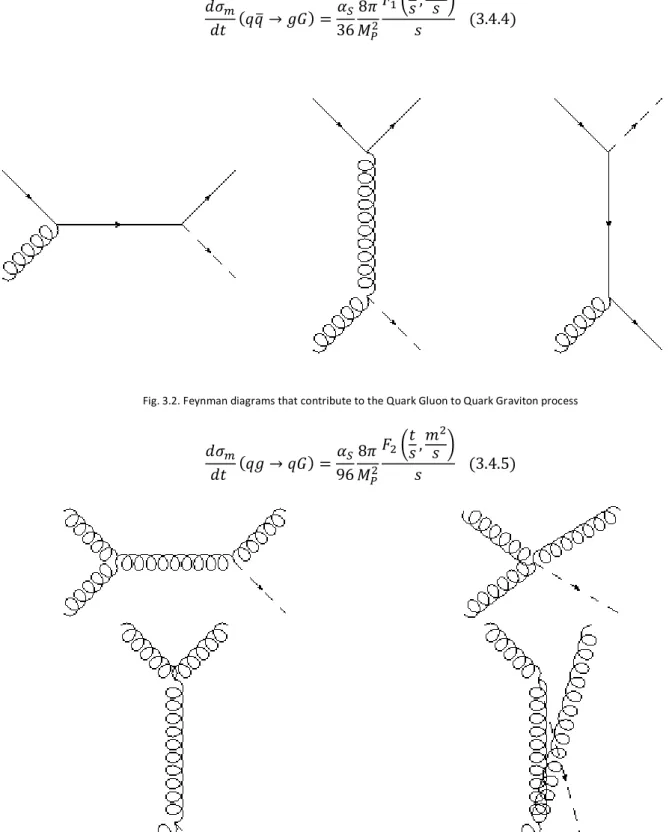
37 𝑑𝜎𝑚 𝑑𝑡 (𝑞𝑞� → 𝑔𝐺) = 𝛼𝑆 36 8𝜋 𝑀_𝑃2 𝐹1�𝑡𝑠 ,𝑚 2 𝑠 � 𝑠 (3.4.4)

Fig. 3.2. Feynman diagrams that contribute to the Quark Gluon to Quark Graviton process

𝑑𝜎𝑚 𝑑𝑡 (𝑞𝑔 → 𝑞𝐺) = 𝛼𝑆 96 8𝜋 𝑀_𝑃2 𝐹2�𝑡𝑠,𝑚 2 𝑠 � 𝑠 (3.4.5)

Fig. 3.3. Feynman diagrams that contribute to the Gluon Gluon to Gluon Graviton process

𝑑𝜎𝑚 𝑑𝑡 (𝑔𝑔 → 𝑔𝐺) = 3𝛼𝑆 16 8𝜋 𝑀_𝑃2 𝐹3�𝑡𝑠,𝑚 2 𝑠 � 𝑠 (3.4.6) 𝐹 functions are listed in the appendix (section 7.3.1).

38

3.4.3 Expected results

Mono-jet cross section has therefore an additional term equal to the sum of all the previous contributions: ∆𝜎𝐴𝐷𝐷= 𝜎(𝑞𝑞� → 𝑔𝐺)𝑞=𝑢,𝑑,𝑠,𝑐,𝑏,𝑡+ 𝜎(𝑞𝑔 → 𝑞𝐺)𝑞=𝑢,𝑑,𝑠,𝑐,𝑏,𝑡,𝑞�+ 𝜎(𝑔𝑔 → 𝑔𝐺) (3.4.7) 𝜎(1,2 → 3, 𝐺) = � 𝑑𝑚𝑑𝑡𝑑𝑥1𝑑𝑥2 2𝜋 𝛿 2 Γ �𝛿2� 𝑀𝑃2 8𝜋𝑀_𝐷2+𝛿𝑚𝛿−1 𝑑𝜎𝑚 𝑑𝑡 (1,2 → 3, 𝐺)𝑓1(𝑥1, 𝑄)𝑓2(𝑥2, 𝑄) 𝐷 (3.4.8)

3.5 Virtual Graviton Exchange

3.5.1 Scattering amplitudes

In this case scattering amplitudes have the form

𝒜 = 𝒮(𝑠) �𝑇𝜇𝜈𝑇𝜇𝜈−𝑇𝜇 𝜇_𝑇 𝜈𝜈 2 + 𝛿� = 𝒮(𝑠)𝒯 (3.5.1) where 𝒮(𝑠) = 1 𝑀𝐷2+𝛿 � 𝑑𝛿_𝑞 𝑠 − 𝑞2 |𝑞|<Λ = 𝜋 𝛿 2 Γ �𝛿2� Λ𝛿−2 𝑀𝐷2+𝛿ℱ𝛿� 𝑠 Λ2� 𝑠≪Λ2 �⎯⎯� ⎩ ⎪ ⎪ ⎨ ⎪ ⎪ ⎧ 𝜋𝛿/2 Γ �𝛿2� Λ𝛿−2 𝑀𝐷2+𝛿 = 8 𝑀𝒯4 𝛿 > 2 𝜋 𝑀_𝐷4𝐿𝑛 � 𝑠 Λ2� 𝛿 = 2 −𝑖𝜋 𝑀_𝐷3_√𝑠 𝛿 = 1 (3.5.2)

Here Λ is the cut-off energy for perturbation theory to be valid (see section 3.6). ℱ functions are listed in the appendix (section 7.3.2).

3.5.2 Relevant processes Cross sections

The following is from reference [3].

Fig. 3.4. Additional diagram for the Fermion Anti-Fermion to Photon Photon process

𝑑𝜎 𝑑𝑡 �𝑓𝑓̅ → 𝛾𝛾� = 𝜋 16𝑁𝑓𝑠2 �2𝛼𝑞𝐹2− 𝑡𝑢_{4𝜋 𝒮(𝑠)�} 2 𝑡𝑢 (3.5.3)

39

Fig. 3.5. Additional diagram for the Gluon Gluon to Photon Photon process

𝑑𝜎

𝑑𝑡 (𝑔𝑔 → 𝛾𝛾) =

𝑡4_{+ 𝑢}4

512𝜋𝑠2|𝒮(𝑠)|2 (3.5.4)

Fig. 3.6. Additional diagrams for the Gluon Gluon to Gluon Gluon process

𝑑𝜎 𝑑𝑡 (𝑔𝑔 → 𝑔𝑔) = 1 256𝜋𝑠2 ⎣ ⎢ ⎢ ⎡9𝑔𝑠4(𝑠2+ 𝑡2+ 𝑢2)3 2𝑠2_𝑡2_𝑢2 − � �6𝑔𝑠2𝑅𝑒 �𝑡 4_{+ 𝑢}4 𝑡𝑢 𝒮∗(𝑠)� − 𝑢4(4|𝒮(𝑠)|2+ 𝑅𝑒[𝒮(𝑠)𝒮∗(𝑡)] + 4|𝒮(𝑡)|2)� 𝑐𝑦𝑙 𝑠,𝑡,𝑢 ⎦ ⎥ ⎥ ⎤ (3.5.5)

Fig. 3.7. Additional diagram for the Gluon Gluon to Quark Anti-Quark process

𝑑𝜎 𝑑𝑡 (𝑔𝑔 → 𝑞𝑞�) = (𝑡2_{+ 𝑢}2₎ 128𝜋𝑠2 �𝑔𝑠4 (4𝑠2_{+ 9𝑠𝑡 + 9𝑡}2₎ 3𝑠2_𝑡𝑢 − 𝑔𝑠2𝑅𝑒[𝒮∗(𝑠)] + 3 2|𝒮(𝑠)|2𝑡𝑢� (3.5.6) For the inverse process matrix element is the same, it is only necessary to average on quark colors instead of gluon colors, this contributes with a factor (8/3)2

𝑑𝜎 𝑑𝑡 (𝑞𝑞� → 𝑔𝑔) = (𝑡2_{+ 𝑢}2₎ 36𝜋𝑠2 �𝑔𝑠4 (4𝑠2_{+ 9𝑠𝑡 + 9𝑡}2₎ 3𝑠2_𝑡𝑢 − 𝑔𝑠2𝑅𝑒[𝒮∗(𝑠)] + 3 2|𝒮(𝑠)|2𝑡𝑢� (3.5.7) By crossing one may obtain 𝑔𝑞 → 𝑔𝑞, that is exchanging 𝑠 with 𝑡 and multiplying for a factor 8/3 because of the average on the initial states

𝑑𝜎 𝑑𝑡 (𝑔𝑞 → 𝑔𝑞) = (𝑠2_{+ 𝑢}2₎ 48𝜋𝑠2 �𝑔𝑠4 (4𝑡2_{+ 9𝑠𝑡 + 9𝑠}2₎ 3𝑡2_𝑠𝑢 − 𝑔𝑠2𝑅𝑒[𝒮∗(𝑡)] + 3 2|𝒮(𝑠)|2𝑠𝑢� (3.5.8)