2 Design criteria for near-field focused planar arrays

25

2 Design criteria for near-field

focused planar arrays

In this chapter, the basic design criteria for NF focused planar arrays are discussed; design and performance curves are given, as a function of array size, inter-element distance and focal distance [9]-[12]. Firstly, the main parameters used to characterize NF focused antennas are introduced. Then, specific design curves for NF focused square arrays are presented in terms of the most significant design parameters and figures of merit. Then, the above analytical results are validated against a set of numerical data relevant to planar microstrip arrays, obtained by a commercial full-wave electromagnetic solver (Ansoft DesignerTM). The results achieved for NF focused planar arrays are also compared against those presented in earlier works by Hansen [46], [48]-[49] and Sherman [42], which are relevant to electrically large continuous aperture antennas.

2.1

Near-field focused planar square arrays

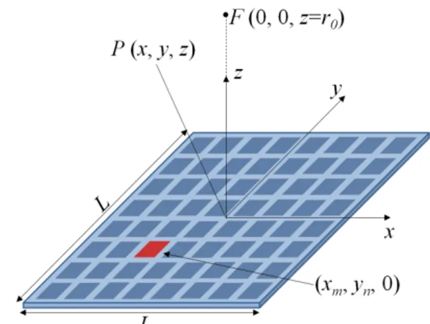
The geometry of a square planar array located in the xy plane of a rectangular coordinate system is shown in Fig. 2.1. The array consists of NxN radiating elements located on a rectangular grid, with an inter-element distance d along both axes. Let us assume L=Nd as the size of each antenna side. The (m,n)-element is located at the point of coordinates (xm, yn, 0), where xm=(2m+1)d/2, yn=(2n+1)d/2, and m and n are integers

26 Fig. 2.1 - 3D view of the planar square array geometry.

The electric field radiated at an observation point P(x, y, z) by the NxN array can be expressed as: 2 1 2 1 2 2 ( ) ( ) N N mn mn m N n N E P I E P      

_{ }

where Imn and Emn(P) are the feeding current and the radiated field corresponding to the

(m, n)-element of the array, respectively. For each element, the feeding current amplitude has been set equal to I0, while its phase φmn has been chosen so that all the

element contributions add in phase at the focal point F=(0, 0, r0) located along the

normal to the array plane:

2 2 2 0 0 2 ( ) mn xm yn r r            (2.2)

where φmn=0 for a conventional EPA. When the focal distance r0 is greater than the

antenna size L the above phase tapering is usually approximated with a quadratic law [46], [49]: mn 









An array made of NxN short dipoles parallel to the x-axis has been considered. Indeed, as it will be later discussed, the antenna element radiation pattern has a negligible effect on the design curves, even for relatively small NF focused arrays. For an x-oriented short dipole, the radiated field can be calculated as:

27





where RiR is the vector going from the element location to the observation point, R is

the distance between the radiating element and the observation point at P, l is the dipole length, and ₀ is the free-space characteristic impedance. It is apparent from eq. (2.3) that for each array element we considered only the dipole far-field component; it follows that results we obtained are not valid in that region where the observation points are close to the array elements (2πR/λ<1). On the other hand, for the arrays we considered the above region will be just a small fraction of the near-field region of the whole array. Also, it is worth noting that the parallel-ray approximation cannot be used in eq. (2.1) since we are interested to evaluate the field around the focal point when the latter lies in the array radiating near-field region.

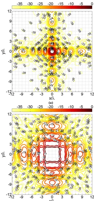
By referring to the array of short dipoles, let us now introduce the characteristic parameters of NF focused antennas, which are quite different from those usually adopted for conventional far-field focused antennas, as anticipated in the previous chapter. Fig. 2.2 shows a sample of the normalized power density radiated by a square array of short dipoles: N=8, d=0.8λ, L=Nd=6.4λ and r0=8.2λ.

In particular, Fig. 2.2a shows the normalized power density radiated by the NF focused planar array at a 12λx12λ square region, lying on the plane parallel to the array and passing through the focal point (transverse plane at z=r0, with r0=8.2λ). To give

evidence to the focalizing effect, the normalized power density radiated on the same plane by an equal-phase array is also presented in Fig. 2.2b. It is apparent from Fig. 2.2a that the lateral size of the -3 dB spot, at the focal plane, can be defined. In particular, for the example we considered, the lateral size of the -3 dB spot region, at z=r0, for the NF

focused array is around λxλ.

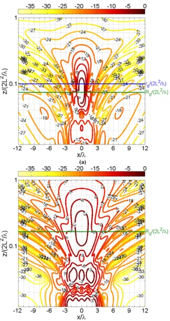
Fig. 2.3 shows the normalized power density radiated by the above 8x8 array at a plane perpendicular to the array aperture and passing through the focal point (longitudinal plane, y=0, E-plane), for both the NF focused array (Fig. 2.3a) and the corresponding EPA (Fig. 2.3b).

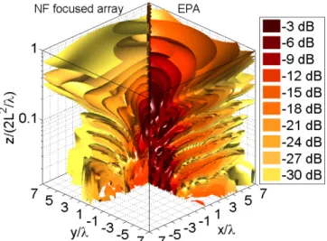
By comparing Fig. 2.2a and Fig. 2.2b (as well as Fig. 2.3a and Fig. 2.3b) it is apparent that a NF focused array can concentrate the radiated power in a limited region near the array aperture, more than a conventional EPA does. This is more evident in Fig. 2.4, where a 3D view of the normalized power density radiated by the 8x8 array of x-directed short dipoles is shown, for both the NF focused array with r0=8.2λ (left hand

28 (a)

(b)

Fig. 2.2 - Normalized power density (dB) radiated by an 8x8 array of x-directed short dipoles (inter-element

spacing d=0.8λ, L=Nd=6.4λ) at a distance z=8.2λ from the array aperture: (a) NF focused array, with r0=8.2λ;

29 (a)

(b)

Fig. 2.3 - Normalized power density (dB) radiated by an 8x8 array of x-directed short dipoles (inter-element

spacing d=0.8λ, L=Nd=6.4λ) on the longitudinal plane at y=0 (E-plane): (a) NF focused array, with r0=8.2λ;

(b) EPA (far-field focused). In both figures, R0 denotes the distance from the array plane of the point where

30

Fig. 2.4 - 3D view of the normalized power density radiated by an 8x8 array of x-directed short dipoles

(inter-element spacing d=0.8λ, L=Nd=6.4λ): NF focused array with r0=8.2λ (left hand side) and EPA (right hand

side).

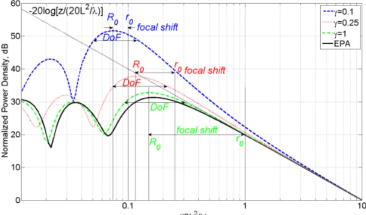
In Fig. 2.5, the normalized power density for the 8x8 array of x-directed short dipoles, evaluated along the direction orthogonal to the array plane (z-axis), is shown for different values of the normalized focal distance r0/λ. In particular, different curves

are plotted corresponding to a set of values of the parameter γ=r0/(2L2/λ) (namely the

focal distance normalized to the far-field region boundary): γ=0.1, 0.25 and 1 (Note that γ=0.1 when r0=8.2λ). A reference curve for the corresponding EPA (namely   ) has 1

also been added. For each curve, the radiated power density is normalized to its value at 10(2L2/λ) which means that the comparison is made for an equal power density (namely, an equal interference level) in the far field. As already known [46], due to the field spreading factor 1/R, the peak of the radiated power density does not occur at the focal point (where all field contributions sum in phase due to the proper aperture phase tapering) but it takes place at a point between the antenna aperture and the focal point (at a distance R0 from the antenna plane).

It is also worth noting that the above shift vanishes for small values of the normalized focal distance γ. On the other hand, when γ>1 the distance R0 rapidly

approaches a limit value corresponding to the case of the EPA: R0/ 2





The Depth of Focus (DoF), which is defined as the distance between the two points along the axis normal to the antenna aperture (z-axis) where the power density is 3 dB

31

below its maximum value, can be extracted from the curves in Fig. 2.5, as a function of the parameter γ.

Each curve in Fig. 2.5 is normalized with respect to the radiated power density at 10(2L2/λ), as this allows to compare the near-field amplitude radiated by the NF focused arrays with respect to that radiated by the conventional EPA, when both radiate the same field amplitude in the far-field region. As expected, the NF focused array is able to radiate a maximum power density that is greater than the maximum power density radiated by the corresponding EPA, when both radiate the same field amplitude in the far-field region. It means that for all those applications where the receiver/target is located in the near-field region of the transmitting antenna, the NF focused array can guarantee a higher power density with respect to an EPA, while still meeting the limits on the maximum far-field radiation (as for example those limits associated to regulations on maximum EIRP). Conversely, for a required field amplitude in the spot region, a NF focused array can guarantee a smaller field in the far-field region, so minimizing interference with nearby radio systems operating at the same frequency band.

Fig. 2.5 - Normalized power density radiated by an 8x8 array of x-directed short dipoles (inter-element

spacing d=0.8λ, L=Nd=6.4λ) along the direction perpendicular to the array plane (on-axis power density). The distance from the array plane is normalized to the far-field region boundary, (2L2/ λ). NF focused array with γ=r0/(2L2/λ)=0.1, 0.25, 1 and  1 (EPA). DoF stands for Depth of Focus.

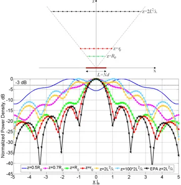
The normalized power density radiated along a direction parallel to the x-axis, at different distances from the array plane is shown in Fig. 2.6 (a sketch of the problem geometry is also shown). As expected [42]-[46], [49], at the focal plane (z=r0) the power

density curve for the NF focused array looks like the far-field radiation pattern of the equalphase array (black continuous line): deep nulls are at the same xlocations, and a -13 dB side lobe level is exhibited. It is also worth noting that the above properties are partially lost along the line passing through the power density peak (z=R0: R0 6.1 when γ=0.1). Moreover, visible pattern degradations appear at points closer to the array plane (z<R0). Finally, it is worth noting that the far-field pattern (z=100(2L2/ λ)) of the

32

NF focused array exhibits a larger beamwidth and higher side lobes with respect to the EPA, which gives explanation for its lower directivity.

Fig. 2.6 - Normalized power density radiated by an 8x8 array of x-directed short dipoles (inter-element

spacing d=0.8λ, L=Nd=6.4λ) along the transverse direction, parallel to the x-axis, at different distances from the array plane.

2.2

Design curves for near-field focused arrays

By resorting to eqs. (2.1)-(2.3), the field radiated by a square array of NxN short dipoles has been calculated, for a set of values of the following parameters: N, d/λ, and γ. The numerical data have been used to construct the curves reported in Fig. 2.7-Fig. 2.10, which are relevant to those physical quantities introduced in the previous paragraph that are useful to design and characterize NF focused arrays. In particular, for each value of γdifferent curves have been plotted in Fig. 2.7-Fig. 2.10 by changing d between 0.4λ and λ, for a set of values of the number of elements N=4, 6, 8, 10, 12, 16, 20. It is important to note that their superposition looks like a single smooth and continuous curve, confirming that each of the physical quantities shown in the above figures is basically a function of the normalized antenna size L/λ=Nd/λ, as expected especially for large arrays. It has also been verified that when d/λ>1, more than one spot region can appear, in a way similar to the appearance of the grating lobes in the far-field

33

radiation pattern of any uniformly-spaced array. Moreover, it should be underlined that arrays smaller than 4x4 are not effective in a focusing process.

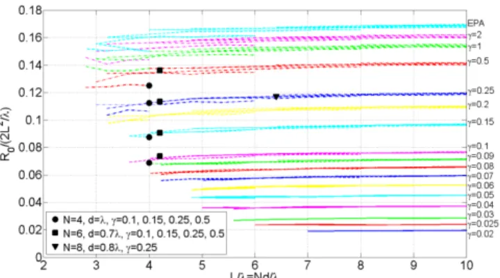
In Fig. 2.7, the normalized distance from the array aperture to the point where the power density reaches a maximum, R0/(2L2/λ), is shown as a function of the array size

L/λ=Nd/λ, for a set of values of the normalized focal distance, γ. When   , all curves 1 approach the limit value valid for arrays focused at infinity: 2

0 (2 / ) 0.17

R L   . On the

contrary, when γ becomes small, R0/(2L2/λ) approaches a value equal to γ, which means

that the field maximum is overlapping with the focal point (R0 ~r0), as discussed in [46]. The quantity R0/(2L2/λ) appears to be almost independent of the array size [46],

except for small arrays (which are usually employed at the UHF and lower frequency bands). We observe that the curves in Fig. 2.7 are useful to predict the shift between the focal point and the point where the power density peak is actually located.

Fig. 2.7 - Normalized distance of the power density peak from the array plane, as a function of the array size

L/λ=Nd/λand for different values of the normalized focal distance, γ. For a given value of γ, the corresponding data are represented by the superposition of a set of curves each one relevant to a fixed value of N (N=4, 6, 8, 10, 12, 16, 20), but with 0.4<d/λ<1. EPA stands for Equal-Phase Array (namely,  1). Markers are relevant to NF focused microstrip arrays simulated with Ansoft DesignerTM_.

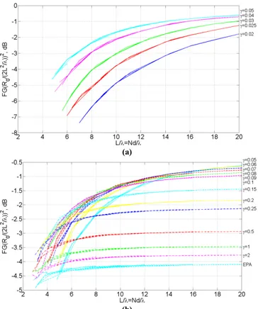
The ratio between the peak power density for the NF focused array and the power density radiated by the corresponding EPA at a distance 2L2/λ from the array aperture can be defined as a Focusing Gain (FG). Curves for the FG are shown in Fig. 2.8 as a function of the array size, and for a set of values of the parameter γ. Specifically, the curves are relevant to the quantity [FG(R0/(2L2/λ))2]dB, where a normalization factor has

been introduced to consider that the normalized power density peak is proportional to 1/R02 for small values of γ [46]. Also, this particular choice allows us to obtain curves

which are confined between an upper bound and a lower bound. The lower bound is that one associated to an EPA and it is approached by those curves with γ>1: for electrically large arrays (Nd  1) this value is close to -4 dB. The upper bound is around -0.5 dB and it is achieved when  ~ 0.05, namely when the focal point is close to the antenna aperture.

34

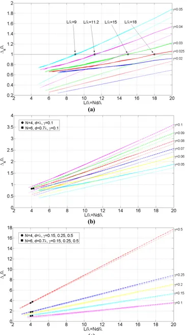
Finally, Fig. 2.9 and Fig. 2.10 show the -3 dB spot diameter (Δs) and the depth of focus (DoF); the first being the spot size in the transverse plane at a distance from the array plane equal to the focal distance.

The -3 dB spot diameter, Δs, has also been compared with the approximate formula given in [42]:

0

0.866 /

s r L

  (2.4)

A good agreement with numerical data is apparent for large values of γγ>0.1; for the above reason, results in Fig. 2.9 are shown up to γ>0.5. By considering the asterisks in Fig. 2.9a where Δs=λ and evaluating the corresponding value of r0/L=γ(2L/λ), it

results that r0/L 0.9; this result is in agreement with [49] where it is shown that for long linear arrays (L=50λ, 500λ) a -3dB spot size equal to the free-space wavelength is obtained when the focal distance is close to the array size, r₀L.

(a)

(b)

Fig. 2.8 - Normalized focusing gain, FG, as a function of the array size L/λ=Nd/λfor different values of the parameter γ: a) γ<0.05 and b) 0.05<γ <2 EPA stands for Equal-Phase Array ( 1).

35

(a)

(b)

(c)

Fig. 2.9 - -3 dB spot diameter Δs (spot size in the transverse plane at the focal distance) as a function of the

array size L/λ=Nd/λ for different values of parameter γ: a0.02<γ<0.05,b0.05<γ<0.1c0.1<γ<0.5The thick lines represent the numerical data and the thin lines those obtained from eq. (2.4). Markers denote performance of NF focused microstrip arrays simulated with Ansoft DesignerTM.

36

Fig. 2.10 - Depth of focus (DoF) as a function of the array size L/λ=Nd/λfor different values of γ. Markers

denote performance of NF focused microstrip arrays simulated with Ansoft DesignerTM.

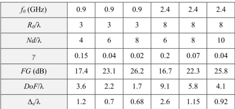
As a sample of the design procedure based on the curves given in Fig. 2.7-Fig. 2.10, the main characteristics of some NF focused arrays are collected in Tab. 2.1.

f0 (GHz) 0.9 0.9 0.9 2.4 2.4 2.4 R0/λ 3 3 3 8 8 8 Nd/λ 4 6 8 6 8 10 γ 0.15 0.04 0.02 0.2 0.07 0.04 FG (dB) 17.4 23.1 26.2 16.7 22.3 25.8 DoF/λ 3.6 2.2 1.7 9.1 5.8 4.1 Δs/λ 1.2 0.7 0.68 2.6 1.15 0.92

Tab. 2.1 - Examples of the estimated performance of some square planar NF focused arrays: operating

frequency, f0; power density peak position, R0/λ array size, L/λ=Nd/λ; focal distance normalized to the

far-field region boundary, γ focusing gain, FG; depth of focus, DoF/λ -3 dB spot diameter, Δs/λ.

The data available at the antenna designer are the operating frequency (or equivalently the free-space wavelength) and the distance from the array plane of the point where a peak of the radiated field is required, R0/λ. By using the curves in Fig. 2.7,

several different pairs (Nd/λ, γ) can be identified, which allow to get the required R0/λ.

Although electrically large arrays are needed to get higher values of the focusing gain, FG, space constraints must be also taken into account (it is worth noting that for a given R0/λ, γ is smaller for larger arrays). Once a pair (Nd/λ, γ) has been chosen, the

normalized amplitude of the power density at R0/λ, FG, can be extracted from the

curves in Fig. 2.8. Finally, the -3 dB spot diameter (at the focal plane) and the depth of focus can be derived from Fig. 2.9 and Fig. 2.10, respectively. It is worth noting that the chosen value of γ is that needed to calculate the phase tapering values in eq. (2.1). By following the above procedure, the values in Tab. 2.1 are obtained. As already noted,

37

better NF focused array performance is achieved with larger antenna size (smaller values of γ). For a given position of the peak power density, R0/λ, a higher focusing gain

can be obtained with a larger array, in a smaller -3 dB spot area.

2.3

Array element radiation pattern

Array performance is apparently dependent on the specific radiating element that is going to be used. On the other hand, authors’ main goal was to get effective design curves and performance data that can be applied (within a certain accuracy degree) almost to any radiating element. Therefore, after constructing design curves by referring to an array of simple short dipoles, it has been needed to demonstrate that the achieved curves were not significantly changing when replacing the radiating element. As a test sample, a square array of microstrip patches has been considered. Moreover, instead of using an approximate analytical radiation pattern (as it was done for the short dipole array), more realistic results from full-wave numerical simulations have been used (Ansoft DesignerTM). In such a way it is possible to take into account how the above single element radiation pattern can affect the NF focused array performance. The microstrip arrays are made of edge-fed square patches (2.94x2.94 cm2 for an operating frequency of 2.4 GHz) printed on a single layer laminate (1.6 mm thick FR4 laminate, with εr=4.4 and tanδ=0.02).

Fig. 2.11 shows the comparison between the analytical results for an array of short-dipoles (eqs.(2.1)-(2.3)) and the simulation results for the patch array (curves with markers). In particular, the curves show the normalized power density evaluated along the direction orthogonal to the array plane (z-axis), for an array with L=Nd=4.2λ dλ). Both an EPA and a NF focused array (γ=0.25) have been considered. For each curve, the radiated power density is normalized to its value at 2L2/λ. Simulated and calculated data differ less than 1 dB, showing that the single element radiation pattern slightly affects the array performance, even for a relatively small array.

Further comparisons are shown in Fig. 2.7 and Fig. 2.9-Fig. 2.10, where the simulation results relevant to three different patch arrays are shown by means of markers: L=Nd=4λarray _{4dλ,circle marker) with γ=0.1, 0.15, 0.25, 0.5;} L=Nd=4.2λarray 6dλsquare marker) with γ=0.1, 0.15, 0.25, 0.5; L=Nd=6.4λ array 8dλ with γ=0.25, which corresponds to the NF focused array designed in [5], triangle marker). A reasonable good agreement between analytical and numerical results is apparent.

Some comparisons with either prototype measurement or simulation results presented in the open literature are also shown, to further check the accuracy of the proposed design curves. In Tab. 2.2, the -3 dB spot diameter extracted from [33] is compared with the design curves in Fig. 2.9c. In [33], two square arrays 4dλ operating at 10 GHz have been designed and characterized with different focal lengths:

38

126 mm (γ=0.13) and 300 mm (γ=0.3). As a sample of the application of our design curves, in Tab. 2.2 we have shown the Δs/λ values obtained by a linear interpolation of those curves in Fig. 2.9c with the γ values nearest to those in [33]: γ=0.1, 0.15 and γ=0.25, 0.5.

Fig. 2.11 - Normalized power density radiated by a 6x6 array (inter-element spacing d=0.7λ L=Nd=4.2λ)

along the longitudinal direction (on-axis power density): analytical data are obtained for an array of x-directed short dipoles, Ansoft DesignerTM _{results refer to a microstrip array, both for a NF focused array (γ=0.25and}

an EPA. f0 (GHz) 10 10 10 10 10 10 L/λ=Nd/λ 4 4 4 4 4 4 γ 0.1 0.13 0.15 0.25 0.3 0.5 Δs/λ - 0.94 - - 1.88 - Δs/λFig. 2.9c 0.9 1.05 1.2 1.6 2.3 3

Tab. 2.2 - Comparison of the -3 dB spot diameter Δs/λbetween measurements on two square NF focused

arrays [33] (N=4, d=λ, γ=0.13, 0.3) and our results in Fig. 2.9c with the closest γvalues: γ=0.1, 0.15, 0.25, 0.5 (the values denoted through a bold character have been obtained by a linear interpolation).

In [36], a method to estimate the behavior of large NF focused arrays through the knowledge of the mutual admittance of smaller subarrays has been presented. In Tab. 2.3, some array parameters extracted from numerical results in [36] are compared with our results from Fig. 2.7, Fig. 2.9 and Fig. 2.10. Although an amplitude tapering is present in NF focused arrays presented in [36], just small differences appear.

For all microstrip arrays we considered, a quite good agreement between analytical, simulation and measurement results has been obtained. A better agreement is expected for larger arrays, for which the array factor becomes the dominant term even in the radiating near-field region. Although the previous validations cannot be exhaustive, it is worth noting that planar microstrip patch arrays are simple but representative examples

39

of radiating element to be used in UHF and microwave implementations of low-cost NF focused planar arrays [5]-[8], [33]-[34].

f0 (GHz) 10 10 L/λ=Nd/λ 8 8 γ 0.15 0.25 R0/(2L2/λ), [36] 0.091 0.122 R0/(2L2/λ), Fig. 2.7 0.095 0.12 Δs/λ, [36] 2 4 Δs/λ, Fig. 2.9c 2.2 3.6 DoF/λ, [36] 11.4 19.1 DoF/λ, Fig. 2.10 13 18

Tab. 2.3 - Comparisons between simulation results of a square planar NF focused array (N=16, d=0.5λ) [36]

and our results (Fig. 2.7, Fig. 2.9 and Fig. 2.10) for different values of normalized focal distance γ: operating frequency, f0; array size, L/λ=Nd/λ; normalized power density peak position, R0/(2L2/λ)focal distance

normalized to the far-field region boundary, γ depth of focus, DoF/λ -3 dB spot diameter, Δs/λ.

2.4

Comparison between near-field focused arrays and focused

apertures

It is well known that the similarities between array antennas and aperture antennas enhance as their electrical size increases. The above statement explains the good agreement between the results of the present NF focused array analysis with those presented in [42]-[47], [49], which are relevant to electrically large NF focused continuous aperture antennas with L  1. For example, curves in Fig. 2.7-Fig. 2.8 tend to become horizontal lines for electrically large arrays, so confirming that the corresponding quantities for electrically large NF focused continuous aperture antennas are almost independent of the antenna size, as predicted by Hansen [46]. The displacement from the above limit values increases when considering electrically small arrays. It follows that the results here presented are more useful for those low-frequency applications where the maximum physical array size is constrained by mechanical and space requirements.

In [46], Hansen showed the normalized power density peak, FG, as a function of R0/(2L2/λ), for large apertures (L≥20λ). Fig. 2.12 shows the curve in Fig. 2.9 of [46],

together with the FG calculated from eqs. (2.1)-(2.3) for a NF focused array of short dipoles with L=Nd=20λ (N=20, d=λ). The two curves are quite close, and little

40

differences are mainly due to the approximations adopted by Hansen when numerically evaluating the radiation integral.

In Fig. 2.12, other two curves have been added, which are relevant to smaller NF focused arrays: L=Nd=10λ (N=10, d=λ), L=Nd=5λ (N=10, d=0.5λ). As expected, for small arrays the differences from analytical results valid for continuous aperture antennas [46] can become not-negligible.

Fig. 2.12 - Focusing gain versus R0/(2L2/λ) for an L=20λ aperture antenna (circle marker, data obtained from

results in [45]) and for a set of NF focused arrays: L=Nd=20λ (square marker) L=Nd=10λ (triangle marker) L=Nd=5λ (star marker).

Finally, to better highlight the advantages of NF focused arrays with respect to conventional far-field focused arrays, in Fig. 2.13 the power density radiated by an 8x8 short-dipole array (d=0.8λL=Nd=6.4λ) is shown for γ=0.1, 0.25, 1 and compared with that one radiated by the corresponding EPA. Differently from the normalization criteria used in Fig. 2.5, the power density radiated by the four arrays are all normalized with respect to the same factor: the power density radiated by the EPA at a distance 2L2/λ. It follows that the different power density levels beyond the far-field region boundary (z=2L2/λ) are related to the directivity differences. The above normalization factor can be estimated as: 2 2 ( 2 ) 16 ( ) ref EPA P S r L D L       _{  }   (2.5)

where DEPA denotes the directivity of a planar array with uniform excitation (both in

phase and amplitude) [50]. From Fig. 2.13 it is apparent that in the far-field region the NF focused array exhibits a lower directivity, as expected due to the phase tapering (the quantity ΔD in the figure is denoted as a positive quantity; for the cases we considered, ΔD=8.7 dB if γ=0.1 and ΔD=1.5 dB if γ=0.25). Then, when comparing the NF focused array and the EPA we can conclude that:

41

 for a given value of the peak power density, in the far-field region the NF focused array will radiate a power density which is around (FG+ ΔD-11) dB less than that one radiated by the corresponding EPA;

 conversely, for a given maximum of the power density radiated in the far-field region, the peak power density radiated by the NF focused array will be (FG+ ΔD-11) dB greater than the power density peak of the corresponding EPA.

Fig. 2.13 - Normalized power density radiated by an 8x8 array of x-directed short dipoles (inter-element

spacing d=0.8λ L=Nd=6.4λ) along the direction perpendicular to the array plane (on-axis power density). For each array the power density is normalized with respect to that one radiated by the EPA at a distance 2L2_{/λThe distance from the array plane is normalized to the far-field region boundary, 2L}2_{/λ. NF focused}

arrays with γ=r0/(2L2/λ)=0.1, 0.25, 1and  1 (EPA).

2.5

Conclusions

The performance analysis of NF focused arrays has been addressed by referring to a planar square array of short dipoles. Based on a simple analytical analysis, design curves and performance data have been obtained for planar square arrays, as a function of antenna size, inter-element distance and focal distance. The above results have been compared with those already known for continuous aperture antennas, as well as with simulation results obtained for planar arrays of microstrip patches. Above comparisons have confirmed the validity of the derived design criteria in feasibility studies of NF focused arrays, even for electrically small arrays. Also, we have shown that design curves are similar to those for continuous aperture antennas only for electrically large apertures. Therefore, design curves and performance data here provided represent a valuable added value with respect to the existing work, when NF focused electrically small arrays are considered. This condition is being frequently met at UHF and lower frequency bands.

Finally, we believe that such design curves can be useful for antenna designers who want to determine in advance the trade-off between performance and complexity of NF

42

focused arrays, in comparison with a conventional far-field focused array (equal-phase array), without waiting for time-consuming full-wave simulations of large arrays.