ALMA MATER STUDIORUM
UNIVERSITA’ DI BOLOGNA
SCHOOL OF ENGINEERING AND ARCHITECTURE
-Forlì Campus-
SECOND CYCLE MASTER’S DEGREE in
INGEGNERIA AEROSPAZIALE/ AEROSPACE ENGINEERING
Class LM20
GRADUATION THESIS
In: Spacecraft Attitude Dynamics and Control
“An optical navigation filter simulator for a CubeSat mission to Didymos
binary asteroid system”
CANDIDATE
Alessandro Casadei
SUPERVISOR
Prof. Dario Modenini
EXAMINER
Prof. Fabrizio Giulietti
A
BSTRACT
The orbital and the attitude control in real-time of an artificial satellite in orbit around a celestial body has been one of the most important aspects of space missions for decades, including those conducted through the use of CubeSats, namely nanosatellites and/or microsatellites of cubic form, increasingly used in space thanks to their simplified structure that requires low costs of design, production and putting into orbit, since the couplings between CubeSats and launchers take place through standardized processes that reduce the hours of work of the designers and offer the possibility of modifying the payload without having to fully re-evaluate the launch project, in addition to the fact that the size of a single CubeSat is so small that allows the launch of multiple nanosatellites simultaneously, going to further reduce the launch costs.
Moreover, the use of a CubeSat often offers the possibility to release it directly into orbit thanks to the transport on a "mother" satellite, necessary in many space missions to put the satellite in communication with the terrestrial operating centers, eventuality that allows further reduction of the launch costs.
Obviously, each CubeSat must be autonomous from the point of view of the production of electrical energy, which usually occurs through the usage of solar panels alternating with accumulators of electricity or batteries for the periods of occultation of sunlight, and from the point of view of navigation, as previously mentioned.
Although the artificial satellites often operate on terrestrial orbits LEO (low Earth orbit) or MEO (medium Earth orbit), for which it is possible to use the assisted navigation through Global Positioning System (GPS) for orbital determination, which requires the availability of a GPS receiver mounted onboard, there exist particular space missions outside the Earth's gravitational field that require autonomous navigation systems in real-time for both attitude control and orbital control. The latter also includes AIDA, the joint NASA-ESA mission that will operate in the 65803 Didymos binary system and whose main purpose is to experiment and investigate the kinetic impact technique for the deviation of the asteroid trajectories in space with a view to a possible collision between one of them and the planet Earth in the future.
HERA, the "mother" satellite designed by ESA in collaboration with other European research institutes, will aim to collect data about the chemical-physical composition of the binary system and about the characteristics of the impact between DART, the bullet-satellite realized and run by NASA together with other US research institutes, and the minor of the two celestial bodies that compose
The "mother" HERA satellite will carry high-level technology onboard, including some CubeSats that will be released when HERA is already in orbit in the Didymos system.
This panorama also includes the DustCube mission, a project proposal for a CubeSat carried out by the Department of Industrial Engineering sited in Forlì (IT) of the University of Bologna in collaboration with other academic and research institutions of the European Union, which the main objective is to assist HERA in the acquisition of data concerning the impact between DART and the minor of the two celestial bodies that form Didymos.
The DustCube mission provides for the need to operate in complete autonomy, communicating in a continuous manner the data collected at HERA, which will send them to the terrestrial operating centers.
The physical configuration of the binary system and the type of mission, which requires the use of infrared cameras, focused on the two celestial bodies that form Didymos, which take pictures of them continuously, lead to prefer the development of an optical navigation filter able to estimate the position and the speed of the CubeSat starting from direction and range measurements with respect to a target body obtained precisely by means of optical technology.
This thesis project, which continues the work done during my curricular internship in the Microsatellite Laboratory of the University of Bologna sited in Forlì (IT), is part of the DustCube project with the aim of investigating in depth the orbital navigation of this CubeSat immersed in the Didymos system and the main one to develop an extended Kalman filter based on optical measurements that allows to simulate the DustCube real-time navigation.
S
OMMARIO
Il controllo orbitale e d’assetto in tempo reale di un satellite artificiale in orbita attorno ad un corpo celeste riveste da decenni uno degli aspetti più importanti delle missioni spaziali, tra cui rientrano quelle condotte tramite l’utilizzo di CubeSats, ovvero nanosatelliti e/o microsatelliti di forma cubica, sempre più utilizzati in ambito spaziale grazie alla loro struttura semplificata che richiede bassi costi di progettazione, di produzione e di messa in orbita, dato che gli accoppiamenti tra CubeSats e lanciatori avvengono tramite processi standardizzati che riducono le ore di lavoro dei progettisti e che offrono la possibilità di modificare il carico utile senza dover rivalutare totalmente il progetto di lancio, oltre al fatto che l’ingombro di un singolo CubeSat è così ridotto da permettere il lancio di più nanosatelliti contemporaneamente, andando a ridurre ulteriormente i costi di lancio.
Inoltre, l’utilizzo di un CubeSat offre spesso la possibilità di un rilascio dello stesso direttamente in orbita grazie al trasporto su un satellite “madre”, necessario in molte missioni spaziali per mettere in comunicazione il satellite con i centri operativi terrestri, eventualità che permette un’ulteriore riduzione dei costi di lancio.
Ovviamente, ogni CubeSat deve essere autonomo dal punto di vista della produzione di energia elettrica, che avviene solitamente tramite l’utilizzo di pannelli solari alternati ad accumulatori di energia elettrica o batterie per i periodi di occultazione della luce solare, e dal punto di vista della navigazione, come accennato precedentemente.
Sebbene spesso i satelliti artificiali operino su orbite terrestri LEO (low Earth orbit) o MEO (medium Earth orbit), per le quali è possibile utilizzare la navigazione assistita tramite Global Positioning System (GPS) per la determinazione orbitale, che richiede la disponibilità di un ricevitore GPS montato a bordo, esistono particolari missioni spaziali al di fuori dal campo gravitazionale terrestre che necessitano di sistemi di navigazione autonoma in tempo reale sia per il controllo d’assetto che per il controllo orbitale.
In quest’ultimo insieme rientra anche AIDA, la missione congiunta NASA-ESA che opererà nel sistema binario 65803 Didymos e che si prefigge come scopo principale quello di sperimentare ed indagare la tecnica di impatto cinetico per la deviazione delle traiettorie degli asteroidi nello spazio in un’ottica di possibile collisione tra uno di essi ed il pianeta Terra in futuro.
HERA, il satellite “madre” progettato dall’ ESA in collaborazione con altri istituti di ricerca europei, avrà come obiettivo quello di raccogliere dati sulla composizione chimico-fisica del sistema binario e sulle caratteristiche dell’impatto tra DART, il satellite-proiettile realizzato e gestito dalla NASA
assieme ad altri istituti di ricerca statunitensi, e il minore dei due corpi celesti che formano Didymos, che dovrebbe avvenire all’incirca nell’Ottobre del 2022.
Il satellite “madre” HERA trasporterà a bordo tecnologia di alto livello, tra cui alcuni CubeSats che verranno rilasciati quando HERA si troverà già in orbita nel sistema Didymos.
In questo panorama rientra anche la missione DustCube, una proposta di progetto di un CubeSat realizzato dal Dipartimento di Ingegneria Industriale con sede a Forlì (IT) dell’Università di Bologna in collaborazione con altri istituti accademici e di ricerca dell’Unione Europea, che ha come obiettivo principale quello di assistere HERA nell’acquisizione dei dati relativi all’impatto tra DART ed il minore dei due corpi celesti che compongono Didymos.
La missione DustCube prevede la necessità di operare in completa autonomia, comunicando in modo continuo i dati raccolti ad HERA, che provvederà all’invio degli stessi ai centri operativi terrestri. La conformazione fisica del sistema binario e la tipologia di missione, che richiede l’utilizzo di fotocamere a raggi infrarossi, puntate sui due corpi celesti che formano Didymos, che scattino immagini degli stessi in modo continuo, portano a prediligere lo sviluppo di un filtro di navigazione ottica in grado di stimare la posizione e la velocità del CubeSat partendo da misure di direzione e di distanza rispetto ad un corpo-bersaglio ottenute per l’appunto tramite tecnologia di tipo ottico. Questo progetto di tesi, che continua il lavoro svolto durante il mio tirocinio curriculare nel Laboratorio di Microsatelliti dell’Università di Bologna con sede a Forlì (IT), si inserisce nel progetto DustCube con l’obiettivo di indagare approfonditamente la navigazione orbitale di questo CubeSat immerso nel sistema Didymos e quello principale di sviluppare un filtro di Kalman di tipo esteso basato su misurazioni ottiche che permetta di simulare la navigazione in tempo reale di DustCube.
C
ONTENTS
LIST OF FIGURES ... X LIST OF TABLES ... XII LEGEND ... XII ACRONYMS ... XIII
INTRODUCTION ... 1
DUSTCUBE’S MAIN FEATURES ... 7
1.1 Operational environment: Didymos system ... 7
1.2 DustCube’s dynamical model ... 10
1.2.1 Reference Frames ... 11
1.2.2 The Circular Restricted 3-Body Problem (CR3BP) for DustCube ... 12
1.2.3 Gravitational attractions acted by Didymain and Didymoon ... 13
1.2.3 The Solar Radiation Pressure (SRP) ... 23
1.2.5 Sun’s gravitational attraction ... 31
DUSTCUBE’S ORBIT PROPAGATOR ... 33
2.1 The Cauchy problem for DustCube’s propagator ... 33
2.2 The Runge-Kutta 4th order method ... 35
2.3 The SPICE Toolkit ... 36
2.3.1 Spice Kernels for DustCube’s orbit propagator ... 37
2.3.2 SPICE’s useful routines ... 38
2.4 Implementation of the orbit propagator ... 39
2.4.1 The Didymos’ Synodic Plane ... 39
2.4.2 The transformation in synodic coordinates ... 41
2.4.3 The orbital propagator’s scripts ... 42
2.4.4 The orbital propagator’s testing ... 49
OPTICAL NAVIGATION ... 56
3.2 Attitude evaluation ... 58
3.3 Image acquiring process ... 59
3.4 Image processing techniques ... 62
3.5 Optical Navigation concept for DustCube mission... 68
KALMAN FILTERING ... 69
4.1 optimal controlling and filtering of dynamic systems ... 69
4.2 Kalman filtering for linear continuous dynamic systems ... 74
4.3 Kalman filtering for linear discrete dynamic systems ... 77
4.4 Linearized Kalman Filter (LKF) ... 81
4.5 Extended Kalman Filter (EKF) ... 84
DUSTCUBE’S FILTER... 87
5.1 The non-linear Dynamic System of DustCube ... 87
5.1.1 The state vector function and its jacobian matrix ... 88
5.1.2 The measurement vector function and its jacobian matrix ... 90
5.1.3 The useful reference frames for the measurements ... 94
5.1.4 The process and the measurement errors ... 96
5.1.5 The covariance error matrices 𝑸𝐬𝐚𝐭 and 𝑹𝐬𝐚𝐭 ... 102
5.2 The Extended Kalman Filter implementation ... 104
5.3 Initial validation of the DustCube’s filter ... 106
5.4 The filtering of the corrupted state of DustCube ... 111
CONCLUSIONS ... 117
APPENDIX ... 119
A.1 Equations of motions... 119
A.1.1 Inertial Reference Frame ... 119
A.1.2 Rotating Reference Frame ... 120
A.1.3 Translating and rotating Reference Frame ... 123
A.1.4 Rotation matrices ... 125
A.2 The Circular Restricted 3-Body Problem (CR3BP) ... 130
A.3 General Cauchy problem... 136
A.4 Statistics for random vectors ... 136
A.4.1 Expected Value: ... 136
A.4.2 Covariance Matrix: ... 137
A.4.3 Correlation Matrix: ... 137
A.4.4 Cross-correlation Matrix: ... 137
A.4.5 Cross-covariance Matrix: ... 138
A.4.6 Gaussian vectors: ... 138
L
IST OF
F
IGURES
Figure i.1: AIDA mission concept infographic (European Space Agency (ESA)) ... 1
Figure i.2: Didymos orbit inside Solar System (Jet Propulsion Laboratory (JPL), NASA) ... 2
Figure i.3: DART Mission Concept (National Aeronautics and Space Admnistration (NASA)) ... 3
Figure i.4: HERA (AIM) Mission Concept infographic (Credits: ESA/Science Office) ... 4
Figure i.5: DustCube CONOPS within Didymos system (Pérez, et al., 2018 (In Press)) ... 5
Figure 1.1: Didymos binary asteroid system (Yu, Michel, Schwartz, Naidu, & Benner, 2017) ... 9
Figure 1.2: The contribution of an infinitesimal element to the gravitational potential ... 14
Figure 1.3: General Legendre functions for 1 ≤ 𝑙 ≤ 6 and 0 ≤ 𝑚 ≤ 𝑙 ... 15
Figure 1.4: Spherical harmonics with 𝑙 = 6 in lateral and prospective views ... 16
Figure 1.5: Legendre functions for zonal (a), sectorial (b) and tesseral (c) harmonics ... 17
Figure 1.6: Didymos and Earth orbits from 11/20/202 (Christian, 2015)1 to 02/20/2023... 23
Figure 1.7: Principles of an illuminated flat plate in prospective view and in top one ... 24
Figure 1.8: Solar flux impinging on DustCube from 2022-06-20 to 2022-11-20 ... 25
Figure 1.9: Conical shadow model (Montenbruck & Gill, Satellite Orbits, 2000) ... 27
Figure 1.10: Illustration of apparent radii and apparent separation ... 28
Figure 1.11: Occultation of the solar disk caused by a spherical body ... 28
Figure 1.12: Occultation of the Sun caused by two spherical bodies ... 30
Figure 2.1: Didymos’ Synodic Plane ... 40
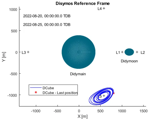
Figure 2.2: DustCube’s parking orbit in L5 from 2022-08-20 to 2022-08-25, considering Didymain and Didymoon as point masses and the SRP contribution ... 44
Figure 2.3: The solar flux which impinges on DustCube from 2022-08-20 to 2022-08-25 ... 45
Figure 2.4: Shadow functions of Didymain and Didymoon from 2022-08-20 to 2022-08-25 ... 45
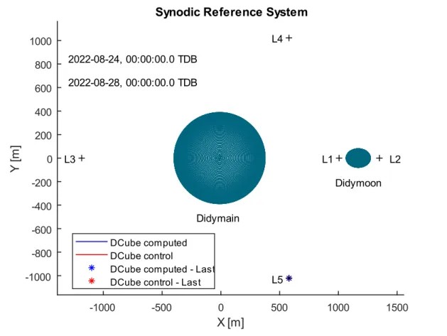
Figure 2.5: Plot of two similar parking orbits in L5 obtained through the MATLAB propagator (blue line) and the Monte Python one (red line), both subjected to central attractions of the primaries and solar gravity ... 51
Figure 2.6: Absolute error trends for the two orbits of Figure 2.5 ... 52
Figure 2.7: Relative percentage error trends for the two orbits of Figure 2.5 ... 52
Figure 2.8: Max absolute, relative and relative percentage errors for the orbits of Figure 2.5 ... 53
Figure 2.9: Plot of two similar parking orbits in L5, obtained by the MATLAB propagator (blue) and the Monte-Python one (red ), due to central attractions of the primaries, solar gravity and SRP w/o sunlight occultations ... 54
Figure 2.10: Max absolute, relative and relative percentage errors for the orbits of Figure 2.9 ... 55
Figure 3.2: Principles of ideal pinhole camera. 𝐚 is the gnomonic projection for a star (Owen,
Methods of Optical Navigation, 2011, February 14) ... 58
Figure 3.3: Principles of emission and detection of light ... 61
Figure 3.4: LOS measurement acquisition using MTI ... 63
Figure 3.5: LOS measurement like stars in the background ... 64
Figure 3.6: CoM achievement using CoB determination technique ... 64
Figure 3.7: CoM achievement using analytic function fitting technique ... 65
Figure 3.8: Limb measurement principle (Polle, et al., 2005, October 17-20)... 65
Figure 3.9: Target viewed as an ellipsoid ... 66
Figure 3.10: Scanning process ... 67
Figure 4.1: Schematic representation of LQR ... 72
Figure 4.2: Kalman Filter’s block diagram ... 80
Figure 4.3: Estimated trajectory of a S/C by using an LKF (Montenbruck & Gill, Satellite Orbits)83 Figure 4.4: Extended Kalman Filter’s block diagram ... 85
Figure 4.5: Estimated trajectory of a S/C by using EKF (Montenbruck & Gill, Satellite Orbits) .... 85
Figure 5.1: Tracking and ranging measurements of a target body ... 91
Figure 5.2: Representation of the longitude λ and the colatitude δ of a generic position vector 𝒓 ... 92
Figure 5.3: Body Reference Frame for DustCube (Aguado, et al., 2016, May 6) ... 94
Figure 5.4: Proposed cameras’ configuration (Aguado, et al., 2016, May 6) ... 95
Figure 5.5: Small deviation errors from the CoM’s pointing of the target body ... 99
Figure 5.6: Corrupted target pointing of a camera mounted onboard a satellite ... 100
Figure 5.7: Estimated state’s error on x ... 108
Figure 5.8: Estimated state’s error on y ... 108
Figure 5.9: Estimated state’s error on z... 109
Figure 5.10: Estimated state’s error on Vx ... 109
Figure 5.11: Estimated state’s error on Vy ... 110
Figure 5.12: Estimated state’s error on Vz ... 110
Figure 5.13: Final estimated state’s error on x ... 112
Figure 5.14: Final estimated state’s error on y ... 113
Figure 5.15: Final estimated state’s error on z ... 113
Figure 5.16: Final estimated state’s error on Vx ... 114
Figure 5.17: Final estimated state’s error on Vy ... 114
Figure 5.18: Final estimated state’s error on Vz ... 115
Figure A.1: The position vector 𝒓 in an Inertial Reference Frame ... 120
Figure A.2: The position vector 𝒓 w.r.t. an Inertial RF and a rotating RF ... 121
Figure A.3: The position vector 𝒓 w.r.t. an Inertial RF and a roto-translating RF ... 124
Figure A.4: The generic 3-Body Problem (3BP) ... 131
Figure A.5: The Circular Restricted 3-Body Problem (CR3BP) ... 132
Figure A.6: Lagrange points in the Synodic Reference Frame ... 134
Figure A.7: Probability density function of a Gaussian random variable with zero mean ... 139
L
IST OF
T
ABLES
Table 1.1: Physical characteristics of Didymos binary asteroid ... 8Table 1.2: Final proposed binary orbit solution for Didymos system ... 9
Table 1.3: Unnormalized exterior spherical harmonic coefficients of Didymain (Takahashi) ... 22
Table 1.4: Unnormalized exterior spherical harmonic coefficients of Didymoon ... 23
Table 2.1: The computed Lagrange equilibrium points of Didymos binary system ... 40
Table 4.1: Kalman Filter algorithm ... 81
Table 4.2: Linearized Kalman Filter algorithm ... 83
Table 4.3: Extended Kalman Filter algorithm ... 86
L
EGEND
• The vectors are written in columns for convenience.
• Symbols in Cambria Math with bold, italic and lowercase characters are VECTORS: 𝒂. • Symbols in Cambria Math with bold, italic and uppercase characters are MATRICES: 𝑨. • Symbols in Cambria Math with no bold characters (lowercase/uppercase) are SCALARS: 𝑎, A. • The words written in blue characters retrieve to other sections of the document.
The digital format of this thesis allows to click on these words to reconnect with the cited section. • The words written in blue and underlined characters recall internet links. The digital format of
this thesis allows the lecturer to click on these words to recover the cited site.
• The words written in grey and italic characters between parenthesis recall citations, figures, equations or demonstrations drawn from references available in bibliography section.
A
CRONYMS
ACRONYM DESCRIPTION
3BP 3-Body Problem
AIDA Asteroid Impact and Deflection Mission
AIM Asteroid Impact Mission
ARE Algebraic Riccati Equation
CoB Center of Brightness
CoM Center of Mass
CONOPS Concept of Operations
COPINS CubeSat Opportunity Payloads CR3BP Circular Restricted 3-Body Problem
CSG Centre Spatial Guyanais
DART Double Asteroid Redirection Test
DLR Deutsches Zentrum für Luft- und Raumfahrt (German Aerospace Center)
DN Digital Number
DRE Differential Riccati Equation DRO Distant Retrograde Orbit
DYD Didymos Reference Frame
ECI Earth-centered Inertial Reference Frame
EKF Extended Kalman Filter
ESA European Space Agency
ET Ephemeris Time
FoV Field of View
GRC Glenn Research Center
GSFC Goddard Space Flight Center
i.e. id est
iff if and only if
INH In-situ Nephelometer
IR Infrared Radiation
ISL Inter-Satellite (radio network) Link ITRF International Terrestrial Reference Frame
JHU/APL Johns Hopkins University Applied Physics Laboratory JPL Jet Propulsion Laboratory
JSC Johnson Space Center
LKF Linearized Kalman Filter
LOS Line of Sight
LQE Linear Quadratic Estimator LQR Linear Quadratic Regulator
LTI Linear Time-Invariant
LTV Linear Time-Variant
MTI Multiple Time Integration
NAIF Navigation and Ancillary Information Facility NAIF Navigation and Ancillary Information Facility NASA National Aeronautics and Space Administration NEXT-C NASA Evolutionary Xenon Thruster - Commercial OCA Observatoire de la Côte d’Azur
ODE Ordinary Differential Equation
OPNAV Optical Navigation
Pdf Probability Density Function
RF Reference Frame
RK4 Runge-Kutta 4th order method
RNH Remote Nephelometer
S/C Spacecraft
SRP Solar Radiation Pressure
SSB Solar System Barycentre
SYN Synodic Reference Frame
TBD To Be Defined
TDB Barycentric Dynamical Time
TOF Time of Flight
UNIBO University of Bologna
UVIGO University of Vigo
w.r.t. with respect to
I
NTRODUCTION
The University of Bologna takes part to AIDA (Asteroid Impact & Deflection Assessment) mission, that is divided in two main independent missions and, consequently, in two main large spacecrafts: • DART (Double Asteroid Redirection Test), that will be the impactor S/C and it is directed by
NASA to the Johns Hopkins University Applied Physics Laboratory (JHU/APL) with support of Jet Propulsion Laboratory (JPL), Goddard Space Flight Center (GSFC), Johnson Space Center (JSC) and other institutions and laboratories;
• HERA, named like the Greek goddess of marriage, that will be the observatory S/C. It has substituted AIM and is directed by ESA with support of German Aerospace Center (DLR), Observatoire de la Côte d’Azur (OCA) and other institutions and laboratories.
The main objective of the AIDA mission (Figure i.1) is to investigate the kinetic impact technique to change the motion of an asteroid in space, which is the selected near-Earth binary system 65803 Didymos (Figure i.2), composed by two celestial bodies, called Didymain and Didymoon.
Figure i.2: Didymos orbit inside Solar System (Jet Propulsion Laboratory (JPL), NASA)
Obviously, the goal will be accomplished by divided the tasks into the two independent missions. Therefore, the main objectives of DART mission are:
1. to test the technologies developed to accomplish a rendezvous with a binary asteroid system, such as autonomous navigation and targeting, reducing the key risks;
2. to demonstrate the kinetic impact technique to change the motion of realistic scale asteroid, crashing into Didymoon with proper angle and velocity, in order to look for possible solutions to deflect asteroids in future events of close encounters with the Earth;
3. to improve impact models by comparing the motion of Didymoon in post-impact phase to one predicted in pre-impact phase;
4. to refine CONOPS for deflection missions.
Consequently, the main goals of the HERA mission are:
1. to acquire data about the deflection of Didymoon and about the cloud of dust generated by its collision with DART spacecraft;
2. to investigate the deep-space optical communication technology and the inter-satellite network ling between CubeSats and a lander;
3. to study the interior structure of an asteroid;
4. to investigate the formation of binary asteroid systems and, more in general, the formation processes of our Solar System.
DART is considered as the first test in a Planetary Defense Technology Demonstration Plan.
It will be launched in January 2021, it will escape from the Earth’s sphere of influence in August 2021 and will crash into Didymoon in October 2022 (see Figure i.3).
For the launch window, DART will utilize the NEXT-C thruster, that is the next generation system based on the Dawn spacecraft propulsion system, developed by Glenn Research Center (GRC) in Cleveland, Ohio, USA.
NEXT-C will exploit solar electric propulsion system as its primary in-space propulsion one, so that it will be able to obtain significant flexibility for the mission timeline, to extend the launch window and to decrease the cost of the launch vehicle.
DART will intercept Didymoon with the aim of an onboard optical camera and an autonomous navigation software and it will crash into the asteroid at an approximated velocity of 6 km/s, changing its motion after collision.
The HERA spacecraft, which was named AIM (acronyms of Asteroid Impact Mission) in the first developing steps, will be launched in October 2020 from the Guiana Space Center (CSG) situated in Kourou, a city of the French Guiana, using an Ariane 6.2 rocket, so that it should enter in the gravity field of Didymos in May 2022 (Figure i.4).
Figure i.4: HERA (AIM) Mission Concept infographic (Credits: ESA/Science Office)
HERA is planned to carry at least three smaller spacecrafts: Mascot-2 asteroid lander, developed by DLR, and two or more CubeSat Opportunity Payloads (COPINS).
Mascot-2 will be released by HERA in August 2022 and will be directed towards Didymoon, where its landing is expected and where it will establish a radar communication channel with HERA. It will emit low frequency radar waves that will pass through Didymoon from side to side, before reaching HERA, to chart asteroid deep interior structure in pre-impact phase and to determine the variations in structure and surface of Didymoon in the post-impact phase.
The CubeSats will be released in August 2022 too and they will establish inter-satellite radio network through triangulation technique with HERA and Mascot-2.
HERA and the CubeSats will monitor the impact of DART, acquiring data about the change of velocity of Didymoon and its angle of deflection, together with the Earth’s observatories.
After the collision, the emitted cloud of dust will be analysed by HERA using thermal images, obtaining important info about the type of debris ejected, their amount, the dimensions of the cloud, its ultimate distance reached and the shape and dimensions of the crate.
The collected data will be continuously sent to the Earth’s observatories by using high-resolution laser communication.
The Department of Industrial Engineering of University of Bologna (IT) sited in Forlì, in collaboration with the Department of Telecommunication Engineering of the University of Vigo (ES) and the MICOS Engineering GmbH of Dübendorf (CH), developed the DustCube mission concept (Figure i.5), one of the five proposals that were selected by ESA for further study, that has the objective to design a 3U CubeSat platform with the main goal to measure the size, shape and concentration of fine dust ejected in the aftermath of the collision and its evolution over time, acquiring speeds of dust particles.
Figure i.5: DustCube CONOPS within Didymos system(Pérez, et al., 2018 (In Press))
Also, DustCube will help HERA to acquire data about physical characteristics, shape and quantity of the plume ejected during DART’s impact by exploiting two light scattering Nephelometer, the remote one (RNH) and the in-situ one (INH), and it will test in orbit a new technique of laser altimetry, using the RNH for time of flight (TOF) measurement (Pérez, et al., 2018 (In Press)).
It will be released by HERA in August 2022 and since it will operate autonomously after the ejection, it will have to be independent for the navigation phases and for the acquisition of data ones, therefore an optical navigation system has been selected: a double IR camera configuration captures
simultaneous images of the two celestial bodies to perform triangulation and to determine the relative position of the S/C w.r.t. them.
The objective of my work of thesis is to develop an optical navigation filter simulator for DustCube in MATLAB programming, starting from a proper propagation of its state.
The thesis is organised as follows:
- Chapter 1 gives a more in-depth overview of DustCube mission, mainly the features of Didymos asteroid and the implemented dynamic model, which considers several levels of disturbances acted on DustCube;
- Chapter 2 presents the DustCube’s state propagator developed though MATLAB programming; - Chapter 3 describes the optical navigation technique, such as the link between optical
measurements and the state/attitude of a S/C, the image acquiring and processing techniques and the selected concept for the optical navigation of DustCube;
- Chapter 4 deepens the Kalman filtering technique, that will be the selected filter for DustCube because it is the most common in use for space navigation, since it is robust, reliable and it does not request great computational effort;
D
UST
C
UBE
’
S MAIN FEATURES
DustCube will operate in Didymos binary asteroid system with the aim of an autonomous optical navigation system, i.e. a double IR camera configuration that will capture simultaneous images of Didymain and Didymoon.
Its CONOPS (Figure i.5) is composed by five operational phases (Pérez, et al., 2018 (In Press)): 1. Birthing phase: DustCube will be released by HERA on August 2022;
2. Injection phase: DustCube will be inserted in a stable orbit at about 3-5 km from the CoM of the system, parking the S/C in a safe region for a time window of 7-14 days to permit early operations, such as the activation of the inter-satellite radio network link (ISL) with the mothership HERA; 3. Pre-impact phase: after the injection phase, DustCube will be transferred to a parking stable orbit
around the L4 or L5 Lagrange equilibrium point (see Figure A.6 in Appendix) of Didymos binary
system, where the S/C will activate the payload operations and will analyse the natural composition and physical characteristics of Didymoon before its collision with DART;
4. Impact phase: during and just after the impact of DART, DustCube will obtain data about the crater, the plume and dust generated by the collision, by using an In-situ Nephelometer (INH) and a Remote Nephelometer (RNH).
The acquisition phase will continue for a maximum of 4 days.
After that, DustCube will rendezvous with Didymoon from the parking orbit (L4 or L5) to the Distant Retrograde Orbit (DRO), an orbit at low altitude around Didymoon, where the S/C will remain for 24 days to acquire high-resolution images and measurements;
5. Post-impact phase: DustCube will be transferred from the DRO to the parking orbit (L4 or L5) to accomplish post-impact operations until the end of the mission.
To complete the mission, a detailed knowledge of the operational environment of DustCube and, therefore, of the forces acting on it is crucial, since the real-time dynamic filter requires a precise computation of the state (eq. (A.1) in Appendix) of DustCube.
In this chapter will be presented the main features of DustCube mission.
1.1
O
PERATIONAL ENVIRONMENT:
D
IDYMOS SYSTEMAs said before, the selected asteroid for AIDA mission is 65803 Didymos, a near-Earth binary asteroid discovered in 1996 by Spacewatch, a group of the University of Arizona’s Lunar and Planetary
Laboratory founded in 1980 with the purpose to explore the various populations of small bodies in the Solar System to study the statistics of asteroids and comets in order to investigate the dynamical evolution of the Solar System.
The choice is not casual: it is more convenient to test the kinetic impact technique in a binary system instead of an individual asteroid, moreover Didymos will pass at the distance of just 11 million kilometers from Earth in 2022, facilitating the communications between HERA and Earth’s bases and the measurements carried out by Earth’s observatories.
Didymos belongs to the Apollo asteroids family, which includes asteroids with semi-major axis greater than 1 AU and perihelion lower than 1.017 AU, such as the Apollo asteroid.
In Table 1.1 are shown the major physical characteristics of the binary system.
Official name of asteroid 65803
Diameter of Didymain 780 m +/- 10%
Diameter of Didymoon 163 m +/- 18 m
Bulk density of Didymain and Didymoon (assumed equal) 2104 kg m-3 +/- 30%
Approximated Didymoon dimensions as= 103 m |bs= 79 m |cs = 66m
Distance from CoM of Didymain and CoM of Didymoon (𝑎𝑜𝑟𝑏) 1180 m +40/-20 m
Total mass of system 5.278e11 kg +/- 0.54e11 kg
Mass ratio Didymoon/Didymain 0.0093 +/- 0.0013
Rotation period of the primary 2.26 h +/- 0.0001 h
Heliocentric eccentricity e e = 0.383752501 +/- 7.7e-9
Heliocentric semimajor axis 𝑎 1.6444327821 +/- 9.8e-9 AU
Heliocentric inclination to the ecliptic 𝑖 3.4076499° +/- 2.4e-6°
Table 1.1: Physical characteristics of Didymos binary asteroid
An observation campaign performed by the Discovery Channel Telescope on 2015-04-13 favors the retrograde orbit solution, with a synchronous rotation of Didymoon around Didymain (Aguado, et al., 2016, May 6), i.e. Didymoon rotational period is the same as Didymoon orbital period.
It is possible to assume that Didymain spin pole is the same as orbital spin pole, although it is important to remark that observations indicate that 25% of near-Earth asteroid binaries have non-zero inclinations (Scheirich & Pravec, 2009).
In Table 1.2 is shown the final proposed binary orbit solution, while in Figure 1.1 is possible to visualize the schematic representation of the Didymos system, where it is easy to recognize the rotation axis od Didymain and the motion of revolution of Didymoon around it.
Pole solution λ=310°, β=-84°
Obliquity to the heliocentric orbit 171° +/- 9°
Diameter ratio Didymain/Didymoon 0.21 +/- 0.01
Didymoon orbital period 𝑻𝑜𝑟𝑏 11.920h +0.004/-0.006
Didymoon orbital eccentricity 𝑒𝑜𝑟𝑏 0.03
Didymoon orbital inclination 𝑖𝑜𝑟𝑏 (assumed) 0°
Obliquity of the primary principal axis w.r.t. the mutual orbital
plane (assumed) 0°
Obliquity of Didymoon principal axis with respect to the mutual
orbital plane (assumed) 0°
Table 1.2: Final proposed binary orbit solution for Didymos system
Figure 1.1: Didymos binary asteroid system (Yu, Michel, Schwartz, Naidu, & Benner, 2017)
The masses and, consequently, the standard gravitational parameters of Didymain (D subscript) and Didymoon (d subscript) can be computed from their diameter ratio, their mass ratio and the total mass of the system, assuming same and homogeneous density (Zannoni, et al., 2018), i.e.:
Md= 4.866 × 10⁹ kg 𝜇D = GMD = 3.4903 × 101m3⁄ s2
𝜇d = GMd = 3.23 × 10⁻¹ m3⁄ s2
Where G is the Universal Gravitation constant: G = 6,67 × 10⁻¹¹(N m2) kg⁄ 2.
Since the ratio between the masses of Didymoon and Didymain is equal to 0.93%, the CoM of the system is very close to the geometric center of Didymain, with an offset of about 10 meters.
The Didymos heliocentric orbit has been uploaded in my software by exploiting the Small Body Database Browser of JPL, which contains the ephemerides of Didymos in a wide time window that covers the entire phase of AIDA mission.
1.2
D
USTC
UBE’
S DYNAMICAL MODELThe dynamical model of DustCube determines the evolution in time of its state (eq.(A.1) in Appendix), which is a vector of six components representing the position vector 𝒓(t) and the velocity vector 𝒗(t) w.r.t. the CoM of the exploited RF.
Since DustCube will be immersed in a binary system, it is possible to consider the estimation problem of the orbit of DustCube as a 3-Body Problem, i.e. the study of the behaviour of the dynamics of an isolated system composed by three punctual bodies of known masses moving due to the reciprocal gravitational attraction, perturbated by external forces that can be considered as disturbances for the isolated system.
Therefore, the most suitable solution is represented by the Circular Restricted 3-Body Problem (see section A.2 The Circular Restricted 3-Body Problem (CR3BP) in Appendix), which simplifies the general 3-Body Problem by assuming that one of the three bodies, the S/C, has a negligible mass, that is the same to recreate the actual situation in which the satellite does not affect the motion of the primaries, which revolve on a Keplerian orbit around their common CoM, so that the study of the dynamics is reduced to the analysis of the motion of the third body, DustCube, moving in a system composed by two massive bodies, Didymain as primary and Didymoon as secondary, with supposed known states.
This approximation is also valid for the masses of HERA, Mascot-2 and the other CubeSats, which can be considered as negligible w.r.t. the total mass of the system.
Since the masses of Didymain and Didymoon are insufficient to hold an atmosphere and to create a magnetosphere, we can compute the state of DustCube by considering a basic dynamical model due to the central attractions of Didymain and Didymoon, expanding and refining the solution step by step through the addition of the following contributions:
• gravitational attraction acted by Didymain by considering its spherical harmonics; • gravitational attraction acted by Didymoon by considering its spherical harmonics; • force generated by the Solar Radiation Pressure (SRP);
• gravitational disturbance of Sun.
Obviously, specific reference frames must be defined for the computation of the state of DustCube. 1.2.1REFERENCE FRAMES
It is important to define proper reference frames to consistently compute the state of DustCube: • ECLIPJ2000 (EC subscript): is an inertial RF centered in SSB, with the x-axis directed towards
the vernal equinox (intersection between the Earth’s equatorial plane and the ecliptic one) at epoch J2000, that stands for 01/01/2000 at 12:00:00 TDB, the z-axis perpendicular to the mean ecliptic plane at epoch J2000 and the y-axis that completes the right-hand frame.
In alternative to ECLIPJ2000, is possible to use the J2000 RF, an inertial RF centered in SSB, with the x-axis directed towards the vernal equinox at epoch J2000, the z-axis perpendicular to the Earth’s mean equatorial plane at epoch J2000 and the y-axis that completes the right-hand frame;
• Didymos Reference Frame (DYD subscript): is the RF linked to the CoM of the binary system with a fixed orientation in space, i.e. it can be considered as a quasi-inertial RF for a steep time-window, since it follows the CoM of the binary system w/o rotating w.r.t. the ECLIPJ2000 RF. The x-y plane coincides with the mean orbital plane of the mutual orbit of Didymain and Didymoon, with the x-axis parallel to the line of nodes and directed towards the ascending node (N-axis), the z-axis directed as the first integral of motion (h-axis) and the y-axis which completes the right-hand frame.
• Didymain quasi-inertial Reference Frame: is the quasi-inertial RF linked to the Didymain’s CoM, that can be considered as coincident with its geometric center, with a constant orientation in space and in time, which can be indifferently choose like the ECLIPJ2000 RF’s one or like the Didymos
RF’s one, so that this frame simply follows the CoM of Didymain w/o rotations;
• Synodic Reference Frame (SYN subscript): is the Synodic RF (Figure A.6 in Appendix) related to Didymos, co-rotating with the binary system. It is centered in the CoM of Didymos, with the x-axis directed as the line of conjunction from Didymain to Didymoon, the z-x-axis directed as the first integral of motion (h-axis) and the y-axis that completes the right-hand frame.
This RF rotates w.r.t. to Didymos RF with an angular speed equal to the mean angular speed of the binary system.
(1.2) The x-y plane is the mean orbital plane of the mutual orbit of Didymain and Didymoon;
• Didymain-fixed Reference Frame (DM subscript): is the body-fixed RF of Didymain, centered in its CoM, that coincides, for simplicity, with its geometric center. The x-y plane is parallel to one containing the mutual orbit of Didymain and Didymoon and the z-axis is directed as the first integral of motion (h-axis), since it can be considered as the rotation axis of Didymain too. This frame rotates around the z-axis with an angular speed equal to the mean rotating speed of the massive body. The x-axis is directed as the ECLIPJ2000’s x-axis at epoch J2000;
• Didymoon-fixed Reference Frame (dm subscript): is the body-fixed RF of Didymoon, centered in its CoM, that is, for simplicity, its geometric center. The x-y plane is parallel to one containing the mutual orbit of Didymain and Didymoon and the z-axis is directed as the h-axis, since it can be considered as the rotation axis of Didymoon too. This frame rotates around z-axis with an angular speed equal to the mean rotating speed of the massive body, that is the mean orbiting speed of Didymoon around Didymain, since the binary system shows a synchronous rotation of Didymoon (Aguado, et al., 2016, May 6). The x-axis is directed as the ECLIPJ2000’s x-axis at epoch J2000.
1.2.2THE CIRCULAR RESTRICTED 3-BODY PROBLEM (CR3BP) FOR DUSTCUBE
As said before, the first useful step is to compute the state of DustCube by exploiting the CR3BP (see section A.2 The Circular Restricted 3-Body Problem (CR3BP) in Appendix), i.e. by considering the mass of DustCube as negligible w.r.t. the masses of the primaries, which are approximated like punctual bodies with no shape.
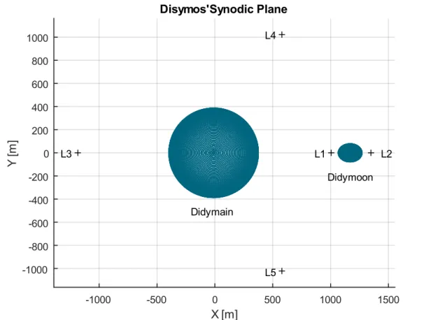
The most useful Reference Frame to visualize the orbit of DustCube is the Synodic one (Figure A.6), which admits five equilibrium points, the so-called Lagrange points L𝑖 (𝑖 = 1, … , 5), in which the velocity and the acceleration of the S/C are null if we consider only the gravitational attractions exerted by Didymain and Didymoon as point-masses.
Therefore, referring to Didymos Reference Frame and defining 𝒓satDYD(t), 𝒓DDYD(t) and 𝒓dDYD(t) as the position vectors of DustCube, Didymain and Didymoon, respectively, w.r.t. the CoM of the binary system, we can compute the position vectors of the S/C w.r.t. Didymain and Didymoon:
𝒓sat−D(t)|DYD≝ 𝒓satDYD(t) − 𝒓DDYD(t) 𝒓sat−d(t)|DYD≝ 𝒓satDYD(t) − 𝒓dDYD(t) ,
so that, it is possible to express the gravitational acceleration acting on DustCube by exploiting the Newton's Law of Universal Gravitation, i.e. by using the equation (A.55):
(1.4) (1.3) 𝒂satDYD(t) = − 𝜇D
‖𝒓sat−D(t)|DYD‖3𝒓sat−D(t)|DYD−
𝜇d
‖𝒓sat−d(t)|DYD‖3𝒓sat−d(t)|DYD
Indeed, as said before, the Didymos RF can be considered as quasi-inertial, so that the equation (1.3)
can be thought as the absolute acceleration of DustCube in inertial coordinates.
Once the solver has computed the state of DustCube in Didymos RF and has transformed it in synodic coordinates, he should obtain a result which satisfies the conditions of the Lagrange points of the Synodic RF (subscript SYN), i.e. 𝒗satSYN(t) = 𝒂satSYN(t) = 𝟎, that means the S/C would remain steady w.r.t. the Synodic RF if it was parked in one of the five equilibrium points.
1.2.3GRAVITATIONAL ATTRACTIONS ACTED BY DIDYMAIN AND DIDYMOON
The main contributions for the total punctual acceleration of DustCube in terms of orders of magnitude are, obviously, the gravitational attractions caused by Didymain and Didymoon.
In first approximation, is possible to simplify the primaries as point-masses, i.e. considering their masses as concentrated in their CoMs, to compute the DustCube’s acceleration, which brings to the CR3BP, that has been explained in the previous section.
Proceeding with the refinement of the computed solutions, is necessary to account for the actual mass distributions, since the primaries are not punctual and have non-spherical shape.
Therefore, defining the position vector of the satellite w.r.t. the CoM of Didymain or Didymoon in body-fixed RF (b subscript) like 𝒓sat(t)|b= (𝑥b(t), 𝑦b(t), 𝑧b(t)), the acceleration of DustCube due to gravitational attractions of the primaries is derived by its gravitational potential UsatG|
b, i.e.: 𝒂satG(t)| b= 𝑑2𝒓sat(t) 𝑑t2 | b
= 𝛁[UsatG(𝒓sat(t))] b=
𝜕UsatG(𝒓sat(t))
𝜕𝒓(t) |
b
In case of the bodies are considered as point-masses, applying the relation (1.4) for both the primaries in their body-fixed RFs and summing up the two contributions, the computed DustCube’s acceleration simply becomes the already mentioned eq. (1.3), which represents the acceleration due to central attractions of the primaries.
Developing the state propagator for more precise computations, we must redefine the gravitational potential by considering the actual shapes and mass distributions of the primaries.
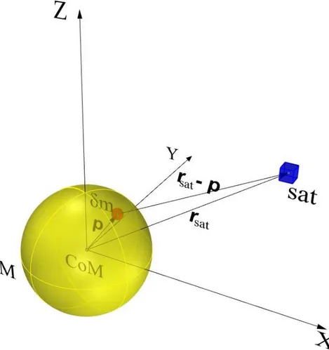
Figure 1.2: The contribution of an infinitesimal element to the gravitational potential
Indeed, starting from the Figure 1.2, we can visualize the gravitational influence of every infinitesimal mass 𝛿m of a generic massive body on the satellite motion.
Defining 𝒑(t)|b as the position vector of 𝛿m w.r.t. the body-fixed RF centered in the CoM of the celestial body, the gravitational potential due to a single primary can be computed by integrating the infinitesimal contributions on the entire domain, which is the body mass M:
UsatG(𝒓sat(t))|b = G ∫
𝛿m
‖𝒓sat(t)|b− 𝒑(t)|b‖ ,
which requires an appropriate evaluation of the inverse of the distance for 𝑟sat(t) > 𝑝(t), i.e.: 1 ‖𝒓sat(t)|b− 𝒑(t)|b‖ = 1 𝑟sat(t) ∑ ( 𝑝(t) 𝑟sat(t) ) 𝑙 P𝑙[cos(𝛾)] ∞ 𝑙=0 ,
where 𝛾 is the angle between 𝒓sat(t)|b and 𝒑(t)|b and P𝑙[cos(𝛾)] is the Legendre polynomial or function of degree 𝑙 for the specific function cos(𝛾).
The generic Legendre polynomial P𝑙 of degree 𝑙 for a scalar function 𝑢 is defined like:
(1.5)
P𝑙[𝑢] ≝ 1 2𝑙 𝑙!
𝑑𝑙
𝑑𝑢𝑙(𝑢2− 1)𝑙 ,
which can be used to obtain the associated Legendre polynomial P𝑙𝑚[𝑢] of degree 𝑙 and order 𝑚:
P𝑙𝑚[𝑢] ≝ (1 − 𝑢2)𝑚2 𝑑 𝑚 𝑑𝑢𝑚P𝑙[𝑢] = 1 2𝑙 𝑙!(1 − 𝑢2) 𝑚 2 𝑑 𝑙+𝑚 𝑑𝑢𝑙+𝑚(𝑢2− 1)𝑙 In Figure 1.3 are shown the general Legendre functions for 1 ≤ 𝑙 ≤ 6 and 0 ≤ 𝑚 ≤ 𝑙.
Figure 1.3: General Legendre functions for 1 ≤ 𝑙 ≤ 6 and 0 ≤ 𝑚 ≤ 𝑙
Introducing the planetocentric latitude and longitude of the satellite 𝜙sat(t) and 𝜆sat(t), respectively, we can expand the generic Legendre polynomial P𝑙[cos(𝛾)] of eq. (1.6) by using some important properties, to finally obtain the gravitational potential of the satellite due to a single massive body in body-fixed RF as a series of Legendre polynomials (Vallado & McClain, 2007, May 5), (Montenbruck & Gill, Satellite Orbits, 2000):
UsatG| b≝ GM 𝑟sat(t)∑ ∑ ( Rp 𝑟sat(t)) 𝑙 P𝑙,𝑚[sin(𝜙sat(t))] 𝑙 𝑚=0 ∞ 𝑙=0
[C𝑙,𝑚cos(𝑚𝜆sat(t)) + S𝑙,𝑚sin(𝑚𝜆sat(t))] ,
where: (1.7) (1.8) (1.9)
• Rp is the mean equatorial radius of the massive body [m]; • C𝑙,𝑚 and S𝑙,𝑚 are unnormalized gravitational coefficients.
The Legendre polynomials P𝑙,𝑚[sin(𝜙sat(t))] and the coefficients C𝑙,𝑚 and S𝑙,𝑚, which characterize the massive body, define the so-called spherical harmonics of degree 𝑙 and order 𝑚, that can be grouped in three main classes:
• Zonal harmonics: 𝑚 = 0 and 𝑙 ≠ 0; • Sectorial harmonics: 𝑙 = 𝑚;
• Tesseral harmonics: 𝑙 ≠ 𝑚, with 𝑙 ≠ 0 and 𝑚 ≠ 0.
The Figure 1.4 displays some examples of spherical harmonics for a generic quasi-spherical massive body while the Figure 1.5 shows the Legendre functions for zonal harmonics, sectorial harmonics and tesseral harmonics, for a maximum degree 𝑙 = 6 and 𝑢 ∈ [−1,1].
(a)
(b)
(c)
Finally, computing the gradient of the gravitational potential of eq. (1.9) in body-fixed coordinates, we obtain the acceleration of the S/C related to a single celestial body.
A useful and quite easy implementation of the accelerations due to gravitational attraction of non-spherical shaped celestial bodies is available in Montenbruck O., Gill E., Satellite Orbits, Springer, 3rd edition, 2005 (Montenbruck & Gill, Satellite Orbits, 2000), which considers the three components of acceleration vector due to spherical harmonics as the sum of partial accelerations computed for every harmonic, namely:
𝑥̈b(t) = ∑ 𝑥̈𝑙,𝑚b(t) 𝑙,𝑚
𝑦̈b(t) = ∑ 𝑦̈𝑙,𝑚b(t) 𝑧̈b(t) = ∑ 𝑧̈𝑙,𝑚b(t) 𝑙,𝑚
𝑙,𝑚
Therefore, defining the useful scalar coefficients V𝑙,𝑚(t) and W𝑙,𝑚(t) as:
V𝑙,𝑚(t)| b≝ (
Rp 𝑟(t))
𝑙+1
P𝑙,𝑚[sin(𝜙𝑔𝑐sat(t))] cos(𝑚𝜆sat(t))
W𝑙,𝑚(t)| b ≝ (
Rp 𝑟(t))
𝑙+1
P𝑙,𝑚[sin(𝜙𝑔𝑐sat(t))] sin(𝑚𝜆sat(t)) ,
is possible to simplify the gravitational potential of eq. (1.9):
UsatG(t)| b= GM Rp ∑ ∑ [C𝑙,𝑚V𝑙,𝑚(t)|b+ S𝑙,𝑚W𝑙,𝑚(t)|b] 𝑙 𝑚=0 ∞ 𝑙=0
The scalar coefficients V𝑙,𝑚(t) and W𝑙,𝑚(t) of eqs (1.11) can be seemed difficult to compute, but since they follow recurrence relations (Montenbruck & Gill, Satellite Orbits, 2000), i.e.:
V𝑚,𝑚(t)| b= (2𝑚 − 1) [ Rp 𝑥b(t) 𝑟(t)2 V𝑚−1,𝑚−1(t) − Rp 𝑦b(t) 𝑟(t)2 W𝑚−1,𝑚−1(t)] W𝑚,𝑚(t)|b= (2𝑚 − 1) [ Rp 𝑥b(t) 𝑟(t)2 W𝑚−1,𝑚−1(t) + Rp 𝑦b(t) 𝑟(t)2 V𝑚−1,𝑚−1(t)] V𝑙,𝑚(t)|b= ( 2𝑙 − 1 𝑙 − 𝑚) Rp 𝑧b(t) 𝑟(t)2 V𝑙−1,𝑚(t) − ( 𝑙 + 𝑚 − 1 𝑙 − 𝑚 ) R2p 𝑟(t)2V𝑙−2,𝑚(t) W𝑙,𝑚(t)| b= ( 2𝑙 − 1 𝑙 − 𝑚) Rp 𝑧b(t) 𝑟(t)2 W𝑙−1,𝑚(t) − ( 𝑙 + 𝑚 − 1 𝑙 − 𝑚 ) R2p 𝑟(t)2W𝑙−2,𝑚(t) , they are easily computable with a recursive implementation, starting from the obvious values:
(1.10)
(1.11)
(1.12)
(1.15) V0,0(t) = Rp
𝑟(t) , W0,0 = 0
Finally, the partial accelerations in body-fixed coordinates become (omitting the time dependence and the body-fixed RF subscript of the scalar coefficients V𝑙,𝑚(t) and W𝑙,𝑚(t)):
𝑥̈𝑙,0b =GM R2p (−C𝑙,0V𝑙+1,1) 𝑦̈𝑙,0b=GM R2p (−C𝑙,0W𝑙+1,1) 𝑥̈𝑙,𝑚b = GM 2R2p[(−C𝑙,𝑚V𝑙+1,𝑚+1− S𝑙,𝑚W𝑙+1,𝑚+1) + (𝑙 − 𝑚 + 2)! (𝑙 − 𝑚)! (C𝑙,𝑚V𝑙+1,𝑚−1+ S𝑙,𝑚W𝑙+1,𝑚−1)] 𝑦̈𝑙,𝑚b = GM 2R2p[(−C𝑙,𝑚W𝑙+1,𝑚+1+ S𝑙,𝑚V𝑙+1,𝑚+1) + (𝑙 − 𝑚 + 2)! (𝑙 − 𝑚)! (−C𝑙,𝑚W𝑙+1,𝑚−1+ S𝑙,𝑚V𝑙+1,𝑚−1)] 𝑧̈𝑙,𝑚b = GM R2p [(𝑙 − 𝑚 + 1)(−C𝑙,𝑚V𝑙+1,𝑚 − S𝑙,𝑚W𝑙+1,𝑚)]
As said before, these partial accelerations are computed in a body-fixed RF centered in the CoM of the celestial body, but the final acceleration must be written in an inertial RF.
So, we must transform the acceleration vector from the body-fixed RF to the inertial one by exploiting the proper rotational matrix and, eventually, the drift between the two CoMs.
For example, considering a S/C orbiting around the Earth, the partial accelerations are computed in ITRF, but the final acceleration vector must be transformed in ECI frame:
𝒂ECI(t) = 𝑻(t)𝒂ITRF(t) ,
where 𝑻(t) is the transformation matrix between ITRF and ECI reference frames.
Obviously, the C𝑙,𝑚 and S𝑙,𝑚 unnormalized gravitational coefficients related to spherical harmonics must be known a-priori, since their computation requires difficult techniques to map the masses distribution of every celestial body considered.
Some publications prefer to adopt the normalized gravitational coefficients C̅𝑙,𝑚 and S̅𝑙,𝑚 instead of the unnormalized ones, since the first normally show lower changes in magnitude between a combination of degree 𝑙 and order 𝑚 and the subsequent one.
It is possible to easily shift from the unnormalized coefficients to the normalized ones, and vice versa, by exploiting the following equations (Montenbruck & Gill, Satellite Orbits, 2000):
(1.14)
(1.17) (1.19) {C̅𝑙,𝑚 S̅𝑙,𝑚 } = √ (𝑙 + 𝑚)! (2 − 𝛿0𝑚)(2𝑙 − 1)(𝑙 − 𝑚)! { C𝑙,𝑚 S𝑙,𝑚} ,
where 𝛿0𝑚 is the Delta of Kronecker function.
The normalized associated Legendre functions are obtainable from the unnormalized ones too, i.e.:
P
̅𝑙,𝑚 = √(2 − 𝛿0𝑚)(2𝑙 − 1)(𝑙 − 𝑚)!
(𝑙 + 𝑚)! P𝑙,𝑚 ,
so that, it is easy to rewrite the gravitational potential of eq. (1.9) by using the normalized coefficients and Legendre functions instead of the unnormalized ones:
UsatG| b≝ GM 𝑟sat(t) ∑ ∑ ( Rp 𝑟sat(t) ) 𝑙 P ̅𝑙,𝑚[sin(𝜙sat(t))] 𝑙 𝑚=0 ∞ 𝑙=0
[C̅𝑙,𝑚cos(𝑚𝜆sat(t)) + S̅𝑙,𝑚sin(𝑚𝜆sat(t))] ,
Obviously, also the partial accelerations computed in eqs (1.15) must be rewritten by considering the normalized gravitational coefficients and Legendre functions.
Although the Montenbruck technique is quite easy to implement and is suitable in terms of computational effort, there exists a better solution to compute the accelerations due to gravitational spherical harmonics, which is the built-in MATLAB function gravitysphericalharmonic, which requires a greater effort to the computational machine than the Montenbruck technique, but it allows more precise solutions.
Since this function has been created to primarily extrapolate the accelerations due to well-known massive bodies in space, such as the Earth, the Moon and so on, for which there exists an excellent knowledge of their shapes and mass distributions, that are already contained inside MATLAB software, is possible to customize the computation process in case of particular celestial bodies by adding the main data available for the orbiting massive body.
Therefore, the calls:
• [ax, ay, az] = gravitysphericalharmonic(r_rot','custom',degree,{'Didymain.mat'@load},'None');
• [ax, ay, az] = gravitysphericalharmonic(r_rot','custom',degree,{'Didymoon.mat'@load},'None'),
allow the user to compute the three components ax, ay, az of the gravitational accelerations due to spherical harmonics in the Planet-Centered Planet-Fixed reference frames by properly specifying the following fields:
- r_rot is the position vector of DustCube w.r.t. Didymain or Didymoon in planet coordinates; (1.18)
- 'custom' suggests to MATLAB to consider the computation as personalized; - degree is the maximum value 𝑙 considered by the MATLAB function;
- {'Didymain.mat'@load} and {'Didymoon.mat'@load} permit to upload the main data of the
celestial bodies Didymain and Didymoon inside the MATLAB function, which are contained in the MATLAB files Didymain.mat and Didymoon.mat, respectively;
- 'None' specifies the action in case of out of range input, which is not in our interest.
The MATLAB files Didymain.mat and Didymoon.mat hold binary data in form of matrices and scalars, which are necessary to properly compute the gravitational acceleration due to the spherical harmonics of the primaries of Didymos.
Every binary file contains the following data of a celestial body: • the mass parameter 𝜇 = GM in [𝑚3⁄ ]; 𝑠2
• the mean equatorial radius Re in [𝑚];
• the maximum degree 𝑙𝑚𝑎𝑥 of the spherical harmonics available for the massive body;
• the matrices C and L of dimensions (𝑙𝑚𝑎𝑥 + 1) × (𝑙𝑚𝑎𝑥 + 1) which hold the normalized exterior spherical harmonic coefficients C̅𝑙,𝑚 and S̅𝑙,𝑚 of the celestial body.
The Didymain’s gravitational acceleration has been tested by using normalized coefficients up to degree 20 and order 20 computed for a homogeneous polyhedronof uniform density by Zannoni M., et al., Radio science investigations with the Asteroid impact mission, Adv. Space Res., 2018 (Zannoni, et al., 2018) and unnormalized exterior spherical harmonic coefficients up to degree 4 and order 4 available from Takahashi Y., Gravity Field Characterization around Small Bodies, University of Colorado, 2013 (Takahashi, 2013), shown in Table 1.3.
The final acceleration of DustCube due to Didymain’s gravitation has an order of magnitude of about 10−5÷ 10−6 [m s⁄ ], even if is important to remark that the major contribute comes from the central 2 attraction C1,0, while the other partial accelerations have orders of magnitude much smaller than the central one.
(1.20) ORDER 𝒍 DEGREE 𝒎 𝐂𝒍,𝒎 𝐒𝒍,𝒎 0 0 1.0 − 1 0 0.0 − 1 1 0 0 2 0 − 6.3422 × 10⁻² − 2 1 0.0 0.0 2 2 4.0949 × 10⁻³ 0.0 3 0 −1.5154 × 10⁻³ − 3 1 2.8455 × 10⁻⁴ 1.1578 × 10⁻⁴ 3 2 2.89891 × 10⁻⁵ −1.89599 × 10⁻⁵ 3 3 3.995 × 10⁻⁴ −1.293 × 10⁻⁴ 4 0 4.66049 × 10⁻² − 4 1 −2.65537 × 10⁻⁵ 3.352119 × 10⁻⁵ 4 2 −9.588539 × 10⁻⁵ −1.28121 × 10⁻⁶ 4 3 −8.305724 × 10⁻⁶ −4.819896 × 10⁻⁶ 4 4 3.544874 × 10⁻⁵ −7.124178 × 10⁻⁶
Table 1.3: Unnormalized exterior spherical harmonic coefficients of Didymain (Takahashi)
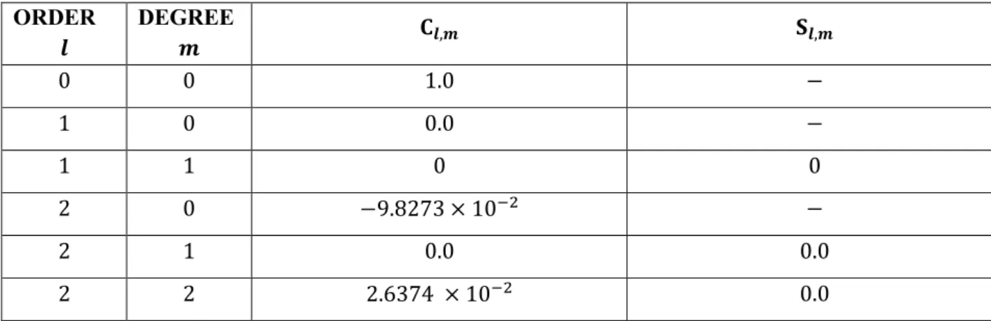
The Didymoon’s gravitational acceleration has been computed by using the degree-2 spherical harmonics expansion of a homogeneous triaxial ellipsoid with these approximated dimensions:
(ad, bd, cd) = (103 m, 79 m, 66 m) ,
by making use of the formulations available from Bills B.G. et al., Harmonic and statistical analyses
of the gravity and topography of Vesta, ICARUS, 2014 (Bills, Asmar, Konopliv, Park, & Raymond, 2014) to compute the unnormalized spherical harmonic coefficients J2 = −C2,0 and C2,2:
J2 = 1 MdR2d (I𝑧−I𝑥+ I𝑦 2 ) = −C2,0 C2,2 = 1 MdR2d (I𝑦 − I𝑥 4 ) ,
where Rd is the mean equatorial radius and I𝑥, I𝑦, I𝑧 are the principal moments of inertia, namely:
I𝑥= Md 5 (bd 2 + c d2) I𝑦 = Md 5 (ad 2 + c d2) I𝑧 = Md 5 (ad 2 + b d 2)
The computed values of the Didymoon’s harmonic coefficients are available in Table 1.4.
(1.22) (1.21)
ORDER 𝒍 DEGREE 𝒎 𝐂𝒍,𝒎 𝐒𝒍,𝒎 0 0 1.0 − 1 0 0.0 − 1 1 0 0 2 0 −9.8273 × 10⁻² − 2 1 0.0 0.0 2 2 2.6374 × 10⁻² 0.0
Table 1.4: Unnormalized exterior spherical harmonic coefficients of Didymoon
The final acceleration of DustCube due to Didymoon’s gravitation has an order of magnitude of about 10−7 [m s⁄ ], where the central attraction stands for the major contribute. 2
Obviously, the gravitational accelerations due to Didymain or Didymoon are computed in body-fixed coordinates and translated in quasi-inertial RF at every iteration.
1.2.3THE SOLAR RADIATION PRESSURE (SRP)
The Solar Radiation Pressure (SRP) contribution must be taken into account, since the acceleration due to it is not negligible during the DustCube mission, when Didymos will pass at a distance of just 0.11 AU from the Earth, as can be seen in Figure 1.6.
(1.23) Simplifying the geometry of the satellite, i.e. considering its shape as a flat plate, is possible to compute the force acting on DustCube due to SRP by exploiting the well-known behaviour of an opaque flat surface subjected to a flow of incoming luminous energy (Figure 1.7).
Figure 1.7: Principles of an illuminated flat plate in prospective view and in top one
Indeed, since the luminous energy that reaches an opaque surface is divided in absorbed, specularly reflected and diffusively reflected, the force acting on a flat plate due to SRP is computable as:
𝒇SRP(t) = −P(t) {(1 − C𝑠𝑝𝑒𝑐)𝒔̂(t) + 2 [C𝑠𝑝𝑒𝑐cos(θ(t)) +1
3C𝑑𝑖𝑓𝑓] 𝒏̂(t)} cos(θ(t)) Atot ,
where:
• P(t) is the momentum flux regard the solar pressure [N/m2];
• C𝑠𝑝𝑒𝑐 is the coefficient of the specular radiation emitted by the illuminated surface; • C𝑑𝑖𝑓𝑓 is the coefficient of the diffusive radiation emitted by the illuminated surface; • 𝒔̂(t) is the unit vector directed from the surface towards the light source;
• 𝒏̂(t) is the unit vector perpendicular to the illuminated surface;
• θ(t) is the angle between 𝒔̂ and 𝒏̂, which is always included between 0° and 90°; • Atot is the approximated area of the illuminated surface [m2].
In our case, since the light source is the Sun and the DustCube’s camera will point towards Didymoon to acquire images during the DART’s impact, the unit vector 𝒔̂(t) will be directed towards the Sun and the versor 𝒏̂(t) towards Didymoon or in the opposite direction, depending on which will be the illuminated surface.
The momentum flux P(t) is a measure of the pressure exerted by the incoming light, therefore it depends on the luminous energy source, the distance from it and the light propagation medium.
(1.24) The last feature affects the speed of movement of the electromagnetic waves while the first two ones are kept in consideration by employing the solar flux Φ(t) [W/m2], which measures the luminous energy that impinges on the surface per unit time and per unit area, namely:
Φ(t) ≝ Ls 4𝜋‖𝒔(t)‖2 ,
where Ls = 3.9 × 1026 [W] is the luminosity of the Sun and ‖𝒔(t)‖ is the distance from the energy source in [m], i.e. the distance between DustCube and the Sun, since 𝒔(t) is defined as the position vector of the last one, considered as a point in space, w.r.t. DustCube’s CoM.
The evolution in time of the solar flux impinging on DustCube during its motion inside Didymos binary system is shown in Figure 1.8, for a time window that spans from midnight of June 20, 2022 to midnight of November 20, 2022, covering five months entirely.
Figure 1.8: Solar flux impinging on DustCube from 2022-06-20 to 2022-11-20
Finally, since Didymos has no atmosphere and no ionosphere, the electromagnetic waves propagate in the vacuum, so that the momentum flux P(t) for DustCube mission (sat subscript) depends on the solar flux (eq. (1.24)) and on the speed of light 𝑐 = 2,99792458 × 10⁸ m/s:
(1.25) Psat(t) ≝Φ(t)
𝑐 =
Ls 4𝜋𝑐‖𝒔(t)‖2
The adimensional coefficients C𝑠𝑝𝑒𝑐, C𝑑𝑖𝑓𝑓 and C𝑎𝑏𝑠 are due to the considered material and are defined as energy ratios, namely:
C𝑠𝑝𝑒𝑐 ≝E𝑠𝑝𝑒𝑐 Etot ; C𝑑𝑖𝑓𝑓 ≝ E𝑑𝑖𝑓𝑓 Etot ; C𝑎𝑏𝑠 ≝ E𝑎𝑏𝑠 Etot
where Etot is the total luminous energy that reaches the opaque surface measured in [J], while E𝑠𝑝𝑒𝑐, E𝑑𝑖𝑓𝑓 and E𝑎𝑏𝑠 are the portions of the total energy that are specularly reflected, diffusively reflected and absorbed, respectively, so that every coefficient is lower than 1.
Therefore, since Etot= E𝑠𝑝𝑒𝑐+ E𝑑𝑖𝑓𝑓+ E𝑎𝑏𝑠, it is enough to know just two coefficients, because the third one can be easily computed by exploiting the obvious relation:
C𝑎𝑏𝑠+ C𝑠𝑝𝑒𝑐+ C𝑑𝑖𝑓𝑓 = 1
Approximating DustCube as a flat plate with no thickness and considering the constrains about materials and payload, we can account for the following rough data:
• msat = 4.365 kg; • Atotsat= 0.09 m2; • C𝑠𝑝𝑒𝑐sat = 0.08; • C𝑑𝑖𝑓𝑓sat = 0.45.
Finally, using the equation (1.23) and the previous data, it is possible to compute the force acting on DustCube due to SRP and the relative acceleration 𝒂satSRP(t) = 𝒇satSRP(t) m⁄ sat.
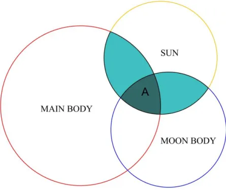
It is important to remark the relation (1.23) does not consider any attenuation factor, but since DustCube will orbit in a binary system, it is needed to take into account the shadows of the two massive bodies: Didymain and Didymoon.
Indeed, making geometric considerations, it is possible to understand the influence of a celestial body on an orbiting S/C in terms of shadow conditions (Figure 1.9).
(1.26)