Radio Occultation experiments of Venus and Mars: similarities and differences

(1)

·ALMA MATER STUDIORUM ·

·UNIVERSIT `

A DI BOLOGNA

_·

SCHOOL OF ENGINEERING -Forl`ı

Campus-SECOND CYCLE MASTER’S DEGREE in AEROSPACE ENGINEERING

Class LM-20

Graduation Thesis in:

Spacecraft Orbital Dynamics and Control

Radio Occultation experiments

of Venus and Mars:

similarities and di↵erences

Candidate:

Edoardo Gramigna

Supervisors:

Prof. Marco Zannoni

Dr. Kamal Oudrhiri

Dr. Marzia Parisi

Dr. Dustin Buccino

Examiner:

Prof. Paolo Tortora

(2)

Acknowledgements

I want to thank my supervisor Professor Marco Zannoni and Professor Paolo Tortora for guiding me throughout these years, and for the opportunity they gave me to work on my Master’s thesis at JPL.

Dr. Kamal Oudrhiri, Dr. Marzia Parisi, Dr. Dustin Buccino and all the Planetary Radar and Radio Sciences Group of Jet Propulsion Laboratory, for their support, their inspiration, and everything they taught me.

My parents Lamberto, Daniela, my sister Annagiulia, my grandparents and my whole family, for always believing in me, my friends Virginia, Gabriele, Gioele and Luis, who shared with me everything about this wonderful journey, Maddalena and all my friends.

(3)

Abstract

In the last decades Venus has not been explored as in the early days of interplanetary missions, yet today the interest has increased and di↵erent space agencies are preparing proposals for future missions. Venus provides a labora-tory next door to our planet to study how rocky planets can form and evolve di↵erently from Earth, even when they start out very similar. Our neighboring planet is the perfect example of what happens in a runaway greenhouse e↵ect, and the state of its atmosphere is interesting in its own right, as it is directly linked to the story of water on the planet and ultimately to the big question of whether life could have arisen beyond Earth. The main purpose of this thesis is the study of the atmosphere of Venus through the radio occultation experi-ments performed by the Venus Express Mission (VEX), sent by the European Space Agency in 2005. In the frame of this investigation comparisons between the Venus atmosphere and Mars atmosphere are shown, in order to highlight the similarities and di↵erences between the two planets. The conclusions de-rived from this work can potentially improve our knowledge and highlight new scientific results about the Venus atmosphere.

(4)

Figure 1: Venus Express mission logo. Credit: ESA

Figure 2: Mars Global Surveyour mission logo. Credit: NASA-JPL

(5)

List of Figures

1 Venus Express mission logo. Credit: ESA . . . iv

2 Mars Global Surveyour mission logo. Credit: NASA-JPL . . . iv

1.1 Venus - Earth - Mars. Credit: NASA . . . 2

2.1 Artist concept of Venus Express. Credit: ESA . . . 8

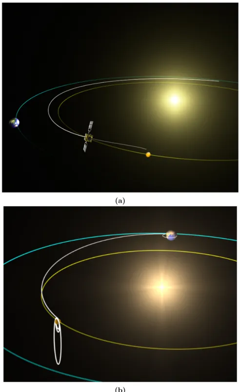
2.2 Interplanetary transfer orbit of Venus Express. Credit: European Space Agency (ESA) . . . 10

2.3 Schematic of launch and transfer orbit. Credit: European Space Agency (ESA) . . . 12

2.4 (a), b) Artist’s impressions of Venus Express journey to Venus. Credit: ESA . . . 13

2.5 Venus Express spacecraft. Credit: ESA . . . 15

2.6 Scientific Instruments carried by Venus Express. Credit: European Space Agency (ESA) . . . 18

2.7 RF communications block diagram. Credit: European Space Agency (ESA) 20 2.8 NASA Deep Space Network Goldstone Complex, California. Credit: NASA 22 2.9 NASA Deep Space Network. Credit: NASA . . . 23

3.1 Ray bending in the atmosphere. r0 = ray path closest approach distance; alfa = deflection angle; a = impact parameter; n=index of refraction. [8] . 26 3.2 Ingress (left) and Egress (right). In this case a star occulted by Venus is represented , but the geometry of the occultation is the same for the space-crafts, too. Credits: https://www.skyandtelescope.com/observing/venus-occults-a-star/ . . . 28

(8)

3.3 Grazing occultation of Aldebaran star by the Moon. As can be seen, the star (or spacecraft) never disappear, it travels slightly above (or under) the planet, so that the signal is always recordable, but weaker due to atmospheric losses. Credits:

http://astroguyz.com/2017/03/31/astro-vid-of-the-week-an-amazing-grazing-occultation/ . . . 28 3.4 Ingress/egress typical processed signal of the occultation occurred the

17th February 2014, recorded by JPL. a) Second past midnight (spm) vs residual frequency: in the middle region the residuals are high and the signal is dominated by noise because the spacecraft was occulted by Venus. b) spm vs Signal to Noise Ratio (SNR), in the middle the noise is dominant, so the SNR decreases. . . 29 3.5 Grazing processed signal of the occultation occurred the 19thMarch 2014,

recorded by JPL. a) Second past midnight (spm) vs residual frequency. b) spm vs SNR: note that with respect to the ingress/egress occultation (Figure 3.4a) the SNR does not decrease as in the previous case, because the spacecraft is not occulted by the planet. The decrease of the SNR is caused by the atmosphere of the planet. . . 31 3.6 Range definition and reference coordinate systems for the spacecraft and

ground station. Credit: NASA . . . 34 3.7 Information about the occultation data 248V EOE20140440325N N N X43RD.1B1

occurred on the 13th _{February 2014. . . 35}

3.8 Signal sampling representation. The continuous signal (green colored line) is replaced by the discrete samples (blue vertical lines). Credit:

https://en.m.wikipedia.org . . . 36 3.9 Outline of the Signal Processing. . . 36 3.10 Sine wave. Credit: https://www.investopedia.com/terms/s/sinewave.asp . 37 3.11 Box function (time domain). Credit: http://www.thefouriertransform.com 38 3.12 Spectrum of the box function. Credit: http://www.thefouriertransform.com 39 3.13 Spectrogram of the VEX radio signal recorded by the DSN on the

ingress/egress occultation of the 7th March 2014. . . 41 3.14 Spectrum and main component frequency of the VEX radio signal at the

xxxx of the 7th _{March 2014. . . 41}

3.15 Noise present in the signal when VEX was occulted by the planet. The FFT algorithm is not able to evaluate the main component frequency because there was no signal coming from the S/C, since it was occulted by Venus. . . 42

(9)

3.16 Signal to Noise Ratio (SNR) of the occultation of VEX on the 13th

February 2014. . . 43

3.17 a) Predicted frequency residuals of the egress occultation of 13th Febuary 2014. b) closer look on a). . . 45

3.18 Examples of Doppler e↵ect. Credit: NASA Science . . . 47

3.19 Examples of SPICE computations. Credit: NAIF, NASA-JPL . . . 48

3.20 Kernels of SPICE. Credit: NAIF, NASA-JPL . . . 49

3.21 Meta-kernel created to analyze the Venus Express data of JPL. . . 50

3.22 a) Reconstructed frequency residuals of the VEX egress occultation occurred the 13th of Februry 2014; b) closer look on the baseline. . . 52

3.23 Frame of reference adopted and geometry for a radio occultation experiment involving transmitter A, receiver B, and target P at the origin of the reference system. . . 54

3.24 SEP angle definition. [15] . . . 69

3.25 Trend of the power spectral density of plasma noise and troposphere noise with respect to the SEP angle. [1] . . . 69

3.26 Elevation angle. [15] . . . 70

3.27 Earth’s atmosphere layers. Credit: https://en.wikipedia.org/wiki/Ionosphere 71 4.1 MATLAB algorithm structure overview. . . 75

4.2 MGS 8361M48A Ingress occultation geometry. . . 79

4.3 Comparison of bending angles vs impact parameters between MATLAB algorithm (left) and Withers (2014) (right), for the MGS 8361M48A occultation. . . 80

4.4 Comparison of the electron density between MATLAB algorithm (left) and Withers (2014) (right), for the MGS 8361M48A occultation. . . 80

4.5 Comparison of the neutral number density between MATLAB algorithm (left) and Withers (2014) (right), for the MGS 8361M48A occultation. . . 81

4.6 Comparison of the refractivity between MATLAB algorithm (left) and Withers (2014) (right), for the MGS 8361M48A occultation. . . 81

4.7 Comparison of the pressure profile between MATLAB algorithm (left) and Withers (2014) (right), for the MGS 8361M48A occultation. . . 82

4.8 Comparison of the temperature profile between MATLAB algorithm (left) and Withers (2014) (right), for the MGS 8361M48A occultation. . . 82

(10)

4.9 Comparison of temperature profiles between MATLAB algorithm (left, with di↵erent boundary condition methods) and P¨atzold (2007) result

(right), for the VEX 234-2006 occultation. . . 83 4.10 Comparison of temperature profiles between MATLAB algorithm (left,

with three di↵erent starting B.C) and P¨atzold (2007) result (right), for the VEX 234-2006 occultation. . . 84 4.11 Temperature-pressure profile obtained for the VEX 234-2006 occultation. 84 4.12 Comparison of temperature profiles between MATLAB algorithm (left)

and P¨atzold (2007) (right) for the VEX DOY 200-2006 occultation a)

Di↵erent B.C methods; b) Three di↵erent B.C, Tellmann [21] method. . . 86 4.13 Temperature-pressure profile obtained for the VEX DOY 200-2006

occultation. . . 87 4.14 a) Temperature profiles for di↵erent integration times ; b) closer look . . 89 4.15 Trend of the power spectral density of plasma noise and troposphere

noise with respect to the SEP angle. [1] . . . 91 4.16 Troposphere seasonal model for calibration. . . 93 4.17 Earth’s troposphere dry seasonal constant term, which adjusts for the

particular DSS used. . . 93 4.18 Earth’s troposphere daily model. . . 93 4.19 Earth’s troposphere daily model for calibration. . . 94 4.20 Earth’s troposphere and ionosphere calibrations for one VEX-JPL

occultation. . . 95 4.21 Earth’s troposphere and ionosphere frequency shifts [Hz] for the VEX-JPL

DOY 066 Ingress occultation. . . 97 4.22 Baseline of the VEX-JPL DOY 070-2014 Ingress occultation. . . 100 4.23 Baseline calibrated of VEX-JPL DOY 070-2014 Ingress occultation. . . . 101 4.24 Baseline not calibrated of MGS DOY 015-2002 Ingress occultation. . . 102 4.25 Baseline calibrated of MGS DOY 015-2002 Ingress occultation. . . 102 4.26 a) Comparison of temperature profiles between relativistic solution (black

line) and non-relativistic solution (red line) for Venus, from VEX JPL

data. b) temperature di↵erence between the two solutions. . . 104 4.27 a) Comparison of temperature profiles between relativistic solution (black

line) and non-relativistic solution (red line) for Mars, from one MGS

occultation. b) temperature di↵erence between the two solutions. . . 105 x

(11)

5.1 Orbits of the two missions. a) Orbit of VEX around Venus, characterized by an apocenter altitude of 66000 km and pericenter altitude of 250 km; b) Orbit of MGS around Mars with an apocenter altitude of 436.5 km

and a pericenter altitude of 372.8 km. . . 108

5.2 Frequency residuals of the occultations. a) VEX Egress DOY 028 2014 ; b) MGS Ingress DOY 361 1998. . . 110

5.3 Closer look of Figure 5.2 on the VEX ionosphere and its baseline. a) Ionosphere of VEX Egress DOY 028 2014 ; b) Baseline VEX Egress DOY 028 2014. . . 111

5.4 Baseline MGS Ingress DOY 361 1998. . . 112

5.5 Electron density profiles. a) VEX Egress DOY 028 2014; b) MGS DOY 361 1998. . . 114

5.6 Neutral number density profiles. a) VEX Egress DOY 028 2014; b) MGS DOY 361 1998. . . 115

5.7 Mass density of neutral atmosphere profiles. a) VEX Egress DOY 028 2014; b) MGS DOY 361 1998. . . 115

5.8 Refractivity profiles. a) VEX Egress DOY 028 2014; b) MGS DOY 361 1998. . . 116

5.9 Closer look on the refractivity profiles. a) VEX Egress DOY 028 2014; b) MGS DOY 361 1998. . . 117

5.10 Bending angle profiles. a) VEX Egress DOY 028 2014; b) MGS DOY 361 1998. . . 118

5.11 Temperature profiles . a) VEX Egress DOY 028 2014; b) MGS DOY 361 1998. . . 119

5.12 Pressure profiles. a) VEX Egress DOY 028 2014; b) MGS DOY 361 1998. 119 5.13 Spatial distribution of occultations data as a function of latitude and longitude. Points are related to the occultation point at 50 km and 25 km altitude for Venus and Mars, respectively. . . 125

5.14 Temperature profiles of the MGS occultations. . . 125

5.15 Pressure profiles of the MGS occultations. . . 126

5.16 Temperature-pressure profiles of the MGS occultations. . . 126

5.17 Temperature profiles for the VEX ingress occultations. . . 127

5.18 Pressure profiles of the VEX ingress occultations. . . 127

5.19 Temperature profiles of the VEX egress occultations. . . 128

5.20 Pressure profiles of the VEX egress occultations. . . 128

(12)

5.22 Temperature-pressure profiles of the VEX ingress occultations. . . 129

5.23 Temperature-pressure profiles of the VEX egress occultations. . . 130

5.24 Tropopause of Venus (example to detect it graphically). . . 133

5.25 Venus’ tropopause temperature vs latitude. . . 134

5.26 Venus’ tropopause altitude vs latitude. . . 134

5.27 Electron density vs altitude, latitude and local solar time (LST). . . 135

5.28 Variation of the 1 bar altitude with respect to: a) Latitude ; b) Subsolar angle. . . 136

(13)

List of Tables

1.1 Venus, Mars, Earth fact sheet. Credit: NASA, ESA . . . 5

5.1 Venus & Mars algorithm’s parameters. . . 122

5.2 Venus egress occultations, NASA-JPL data. . . 123

5.3 Venus Express ingress occultations 2014, NASA-JPL data. . . 124

(14)

(15)

Introduction

Venus is one of the planets visible with the unaided eye so is impossible to say who discovered it first. Venus is the third brightest object in the sky, after the Sun and the Moon, so it is very likely that ancient peoples thousands of years ago knew about this planet. Since it is the planet with the closest approach to Earth, Venus has been the prime target in the early interplanetary exploration. In fact, it is the first planet visited by a robotic spacecraft (Mariner 2 from NASA in 1962), the first planet to be successfully landed on (Venera 7 from the Soviet Union in 1970) and the first planet beyond Earth to be photographed from its surface, made by the lander of Venera 9 mission of the Union Soviet in 1975. Between the 1960s and the 1980s intensive space mission campaigns have been carried out by the Soviet Union and the United States, which sent more than 30 spacecraft, all these missions with the same objective: study-ing the so-called “Earth’s sister”. In fact, Venus revealed similarities in size, density, mass, volume, orbital radius and bulk composition to Earth. However, the similarities ended here, due to the fact that these two planets had evolved in a very di↵erent way: Venus is characterized by extremely high temperatures, pressures, and an atmosphere composition which makes it uninhabitable. Coming back to the space missions, a great contributor in the understanding of the planet was made by the mission Magellan in the early 1990s from NASA, which mapped the gravity but also the entire surface of the planet through a radar instrument, capable to penetrate the thick clouds of the planet [12]. Since then, Venus was largely a forgotten planet for more than a decade as the priority for investigations of the terrestrial planets shifted toward Mars. There were, however, still a large number of fundamental questions to be answered about the past, present and future of our neighboring planet. That is why in 2005, the European Space Agency sent a new mission, the Venus Express Mission (VEX). VEX’s primary objectives were to unveil the unsolved mysteries regarding its atmosphere, the plasma environment and its surface temperatures [20]. Before the mission ended in 2016, the VEX spacecraft sent back a large amount of new scientific data (around 2 Tbit) to Earth

(16)

from the onboard instruments and greatly increased the comprehension of the planet. After Venus Express, the Japanese Space Agency (JAXA), sent a new mission called Akatsuki to Venus, in order to continue the understanding of the planet and the mission is is currently underway. Regarding future space exploration, Venus still represents one of the main targets, since there are still unanswered questions. Interesting proposals from NASA for future space missions at Venus are showing new interests focusing on in-situ missions, since the thick and dense atmosphere of Venus, as well as its temperatures in the middle atmosphere (_{⇠ 75 C at 50 km altitude), makes it a good environment for} this kind of studies, which can enlighten more scientific properties of the planet.

The other Earth’s neighbor is Mars. The Red Planet is the fourth planet from the Sun and the second smallest planet in the Solar System after Mercury. It is usually referred as the Red Planet, due to the e↵ect of the iron oxide which characterize Mars’ surface. This gives it a reddish appearance, which makes it unique among the astronom-ical bodies. The exploration on Mars started in October 1960, with the first Mars probes launched by the former Soviet Union. Unfortunately, both failed. The Americans made the first successful fly-by of Mars with Mariner 4 in July 1965. In particular Mariner 4 captured the first images of another planet ever returned from deep space. After this mission, dozens of robotic spacecrafts as orbiters, landers, and rovers have been sent to the Red Planet by the Soviet Union, United States, European Union and India, to study the planet’s surface, climate and geology. Mars, in fact, has been explored more with respect to Venus. One of the reasons is that the Red Planet is characterized by a thin atmosphere, as well as temperatures and pressures which are not as high as on Venus, so that it has been explored more and in an easier way. In particular not only by orbiters, but by rovers too (which can survive only few minutes on Venus due to the extreme environment). The four rovers sent and landed successfully on Mars until now have been: Sojourner, Opportunity, Spirit and Curiosity. In the summer 2020 two more rovers will be launched to the Red Planet: Mars 2020 by NASA and ExoMars 2020 by the ESA-Roscosmos.

Regarding the history of the radio occultation experiments, the first theories have been presented to the scientific community between the 60’s and 70’s, in particular by Fjeldbo, Eshleman, Phinney, Anderson and Kliore [6]-[7]-[18]-[11]. Then, the first successful experiment has been the one made by the Mariner IV mission, which studied for the first time the atmosphere of another planet, Mars, through a radio occultation investigation. Previous knowledge of the atmospheric properties was poorly defined and

(17)

the vertical profiles have not been accessible to direct Earth-based measurement. After the first successful experiment this kind of studies have been used in several missions to study the atmosphere of other planets (Mariner missions, Cassini, VEX, New Horizons etc).

When the spacecraft is occulted by the planet, the radio signal between the space-craft and the Earth is refracted (or bent) by the planet’s atmosphere, causing a Doppler shift which is detected by the ground stations on Earth. From this Doppler shift is possible to obtain the refractivity index of the atmosphere as well as the vertical profiles of temperature, pressure, electron density and other science characteristics of the planet. This research is focused on the study of the atmosphere of Venus and Mars through radio occultations experiments, in order to highlight similarities, di↵erences and the challenges, both from the engineering and scientific point of view, in performing radio occultation experiments on these planets. In addition, one of the main goals of this work is to obtain new atmospheric results from JPL VEX data never studied before, in order to increase the comprehension and knowledge of Venus’ atmosphere.

This work will cover all the steps needed to investigate radio science data, from the signal processing and its calibration, to the development of an Abel Transform algo-rithm, to the analysis of the vertical profiles of the atmosphere obtained. Regarding the radio science data analyzed within this research: for Venus, the radio occultations data are from the Venus Express mission of 2014, recorded at the Deep Space Network of NASA; regarding Mars, the radio science data are from Mars Global Surveyor (MGS) recorded at the DSN and managed by Jet Propulsion Laboratory.

To conclude, the work is organized as follows: Chapter 1 is dedicated to an overview of the two planets, Venus and Mars, and their atmospheres; Chapter 2 is focused on the Venus Express Mission; Chapter 3 introduces the theoretical background of the radio occultation experiments, the theory behind the Signal Processing and how it has been performed, as well as how to process the radio occultation data: all aspects needed in this research for the scientific comprehension and the engineering formulation of the problems; Chapter 4 shows the development of the atmosphere algorithms for Venus and Mars, its validation, and the di↵erences and challenges due to the calibration of the data; Chapter 5 contains the results obtained for the atmosphere of Venus and Mars, in particular the temperature-pressure profiles will be showed and compared, as well as a Section will be dedicated to the new scientific results obtained for Venus; Chapter 6 is dedicated to conclusions and discussion.

(18)

(19)

Chapter 1

Venus and Mars

Venus is the second planet from the Sun and the closest Earth’s planetary neighbor; from the mythological point of view Venus played a role in many ancient peoples and it owes its name to the Roman goddess of love and beauty. It is similar in structure and size to Earth but Venus spins slowly in the opposite direction from most planets. In addition, it is characterized by a thick atmosphere, which traps heat in a runaway greenhouse e↵ect, making it the hottest planet in our solar system with surface temperatures hot enough to melt lead. From the radio occultation experiment point of view, its thick atmosphere makes the experiments extremely challenging, leading to a strong refraction of the radio signal which travels into it. Glimpses below the clouds reveal volcanoes and deformed mountains.

On the other side, Mars, which is the fourth planet from the Sun and owes its name to the Roman god of war. Mars is a dusty, cold and desert world characterized by a very thin atmosphere. The Red Planet is one of the most explored bodies in our solar system, thanks to its vicinity to Earth and its favorable conditions. Its thin atmosphere per-mits to perform in an easier way with respect to Venus the radio occultation experiments.

Size and Distance

Venus has a radius of 6052 km and it has almost the same size as Earth. The distance with respect to the Sun is on average 108 million km (0.7 AU).

Mars has a radius of 3390 km and in terms of size, is about half of Earth. Its distance to the Sun is on average 228 million km (1.5 AU).

(20)

Venus and Mars

Figure 1.1: Venus - Earth - Mars. Credit: NASA

Formation

Venus and Mars, as its fellow terrestrial planets, have a central core, a rocky mantle and a solid crust, and formed when gravity pulled gas and dust together about 4.5 billion years ago when the solar system settled in its current layout.

Orbit and Rotation

The rotation and the orbit of Venus are unusual. Venus and Uranus are the only ones that rotate from east to west. One full rotation is equivalent to 243 Earth days — the longest day of any planet in our solar system, even longer than a whole year on Venus (225 days). In addition, the Sun doesn’t rise and set each ”day” on Venus like on most other planets. In fact, on Venus one day-night cycle takes 117 Earth days because Venus rotates in the direction opposite of its orbital revolution around the Sun. Its orbit around the Sun is the most circular of any planet (which are more elliptical or oval shaped). To conclude, Venus’ axis of rotation is tilted of 3 degrees, and so the planet does not experience noticeable seasons.

Mars, on the other hand, completes one rotation every 24.6 hours. One year on Mars is made by 669.6 sols (Martian days are called sols) which is equivalent to 687 Earth days. Mars’ axis of rotation is tilted 25 degrees, so it experiences seasons as Earth but longer and di↵erent in length due to its elliptical orbit around the Sun.

(21)

Venus and Mars

Surface

Venus, as seen from space, is bright white because it is covered with clouds that reflect and scatter sunlight. On the other hand, an observer standing at Venus’s surface would see rocks which are di↵erent shades of grey, like the ones on Earth, but the thick atmosphere filters the sunlight so that everything would look orange. Venus has mountains, valleys, and is plenty of volcanoes. The landscape is dusty, and surface temperatures reach 471 degrees Celsius. It is thought that Venus was completely resurfaced by volcanic activity 300 to 500 million years ago.

Mars at the surface is made by brown, gold and tan colors, with temperatures which can range between 20 degrees to -153 degrees Celsius. It appears reddish because of oxidization of the iron present in the rocks, the regolith and the dust. In particular, the dust raises up in the atmosphere, so that from distance makes the planet appear mostly red. Its surface is characterized by volcanoes, impact craters, and extremely big canyons. Mars surface seems to have had a watery past with rivers, deltas and lakebeds. In addition are present rock and minerals that could only have been generated in liquid water. Regarding the water, Mars’ at-mosphere is too thin to permit the existence of liquid water on surface. However, water on Mars as water-ice form is present under the surface in the polar regions.

Atmosphere

Venus’ atmosphere consists mainly of carbon dioxide, with clouds of sulfuric acid droplets. This thick atmosphere traps the Sun’s heat, which is the reason why the surface temperatures are so high. The atmosphere has many layers, each one characterized by di↵erent temperatures. A similar Earth’s surface temperature can be found about 48km up from Venus’ surface. This is the region where fu-ture in-situ missions are planning to set permanent laboratories to study better Venus. The dense atmosphere and the good temperature and pressure at these altitudes, are the best environment for airships, which can increase the knowledge of this planet and its science. Venus is also characterized by extremely fast top-level clouds, driven by hurricane-force winds traveling at about 360 kilometers per hour. Speeds within the clouds decrease with cloud height, and at the surface are estimated to be just a few km per hour. On the ground, the atmosphere is so heavy it would feel like 1.6 kilometers deep underwater.

(22)

Venus and Mars

Mars is characterized by a thin atmosphere, mainly made by carbon dioxide, nitrogen and argon gases, which cannot protect the planet from meteorites, aster-oids and comets impacts. In addition, the atmosphere is so thin that the heat from the Sun easily escapes the planet. Radio occultation experiments performed on Mars are easier with respect to Venus due to the Venus’ thick atmosphere which has a stronger refraction and bending on the radio signal sent by the spacecraft.

Life

No human has visited Venus and the spacecraft that have been sent to the sur-face of Venus did not last very long. Venus’ high sursur-face temperatures overheat electronics in spacecraft in a short time, so it seems unlikely that a person could survive for long on the Venusian surface. The only habitable region it seems to be the one at 50km altitude, characterized by pressure and temperatures not far from the one on Earth.

Regarding Mars, the scientists are not expecting to find living beings but they are looking for signs of life that existed long time ago, when the planet was cov-ered with water, warmer and with a thicker atmosphere, which is one of the main scientific objectives of the Mars2020 NASA mission.

Magnetosphere

Venus’ magnetic field is much weaker than the Earth’s due to Venus’ slow ro-tation, while Mars has no global magnetic field.

Moons and rings

To conclude these main aspects, Venus has no moons, neither rings. Mars has two small moons, Phobos and Deimos but no rings.

(23)

Venus and Mars

Parameter Venus Mars Earth

Average Orbit Distance (km) 108,209,475 227,943,824 149,598,262

Mean orbit velocity (km/s) 35.02 24.07 29.78

Equatorial radius (km) 6,051.8 3,389.5 6,371.00

Equatorial circumference (km) 38,024.6 21,296.9 40,030.2

Volume (km3) 928,415,345,893 163,115,609,799 1,083,206,916,846

Mass (kg) 4.869 x 1024 6.417 x 1024 5.972x 1024

Density (g/cm 3) 5.24 3.934 5.52

Day duration 243 Earth days 24h 37m 23h 56m

Year duration 224.7 Earth days 687 Earth days 365.25 days

Atmosphere 96% CO2 95.32% CO2 78% N2

3.5% N2 2.7% N2 21% O2

1.6% Ar

Escape Velocity (km/s) 10.36 5.03 11.19

Surface Gravity (m/s 2) 8.87 3.71 9.81

Axial Tilt (deg) 177.36 25.2 23.4393

Orbit Inclination (deg) 3.39 1.850 0.00

Eccentricity of orbit 0.00677672 0.093394 0.01671123

(24)

(25)

Chapter 2

Venus Express mission

Venus Express was the first Venus space exploration mission of the European Space Agency (ESA), which between di↵erent mission proposal choose the one of the group led by Dr. D. Titov [22]. Launched on the 9th November 2005 from the Baikonur Cosmodrom, Kazakhstan, it arrived at Venus in April 2006 with the main objective of long-term studies of Venus atmosphere. There were still a large number of fundamental questions to be answered about the past, present and future of Venus, and in addition, it was clear that an improved knowledge of Venus was essential to understand the general evolution of the terrestrial planets in the Solar System. It was with this in mind that ESA and the European scientific community decided to proceed with this new space mission. The mission was proposed in 2001 to reuse the design of the Mars Express mission, with some modifications needed to survive at the extreme thermal environment around Venus, leading to a very cost-e↵ective mission in a very short time [20]. Furthermore, the real innovation with respect to previous missions was a long time period observation, together with a near-polar orbit which was specifically chosen to ensure the maximum scientific return, in particular to study the atmospheric dynamics. Many of the spacecraft’s observations have focused on the structure, dynamics, composition and chemistry of the dense atmosphere and the overlying clouds, but also fascinating and new discoveries have been made, as for example the swirling vortex at the planet’s South Pole, a surprisingly cold region in the high planet’s atmosphere, as well as a high altitude ozone layer and a mysterious layer of sulfur dioxide far above the main cloud layer. In addition, this was the first time that ESA conducted an aerobraking campaign to gain experience for future missions. To

(26)

Venus Express mission

conclude this overview on the mission, thanks to the VEX data, scientists are moving closer toward understanding this enigmatic world, however lot of mysteries are still there. The Akatsuki spacecraft, from JAXA, is currently studying Venus but di↵erent space agencies, as NASA for example, which last Venus space mission was Magellan in 1990, are planning to come back to Venus in the near future.

This chapter will give an overview of the scientific objectives of VEX, its mission operations, the spacecraft, the payload, and the planet Venus, with a particular attention on the description of the onboard radio science experiments.

Figure 2.1: Artist concept of Venus Express. Credit: ESA

2.1 Scientific objectives

The aim of the Venus Express mission was to carry out a comprehensive study of the atmosphere of Venus and to study the planet’s plasma environment and its interaction with the solar wind in some detail. In addition, dedicated surface studies were also performed. The scientific objectives of the Venus Express mission have been concisely expressed within seven scientific themes, which are [20]:

• Atmospheric structure; • Atmospheric dynamics;

(27)

• Cloud layer and hazes;

• Energy balance and greenhouse e↵ect;

• Plasma environment and escape processes;

• Surface properties and geology.

In particular, the first three themes are divided into sub-themes, which refer to the upper (110 km), middle (60 km) and lower parts of the atmosphere (below 60 km).

2.2 Mission Operations

Venus Express was launched by a Soyuz-Fregat launcher from the Baikonur Cos-modrome, Kazakhstan, at 03:33:34 UT on 9 November 2005. First of all, the Soyuz rocket placed the Fregat/spacecraft combination in a suborbital trajectory. Then, a first burn of the Fregat moved the combination into a Low Earth Orbit and, after one orbit around the Earth, the Fregat was fired again, placing the combination in a heliocentric orbit for its interplanetary trajectory. Furthermore, immediately after the second burn, the spacecraft separated from the Fregat and the first au-tomatic activities were carried out, as for example establishing of radio contact with the ground stations, acquisition of the sun-pointing attitude, deployment of the solar arrays. This, followed by commanded activities to prepare the spacecraft for the near-Earth commissioning phase (NECP). The operations descripted above are also called Launch and early orbit phase (LEOP). The next phase was called NECP, which started after the LEOP, and was dedicated to activate and verify the subsystems as well as the payload. Then, after finishing the NECP, the spacecraft was started its interplanetary cruise phase (about 150 days), as can be seen with more details in Figure 2.2, which ended before the Venus Orbit Insertion (VOI).

(28)

Figure 2.2: Interplanetary transfer orbit of Venus Express. Credit: ESA

In this cruise the spacecraft was kept in a three-axes stabilized attitude with the solar arrays facing the Sun and the high gain antenna pointing to the Earth, for daily health checks and navigation. Then, finally, there was the orbit insertion, which started one month before the Venus orbit capture manoeuvre. and ended as soon as the spacecraft reached its operational orbit around Venus. After complet-ing several commanded actions, in order to capture the final orbit, Venus Express started its nominal mission on 4 June 2006. Furthermore, the operational orbit was mainly composed by two activities: the first one with the orbital time (OT, time counted from each pericenter pass) between 2 and 11h for the telecommuni-cations with the Earth; the second one, characterized by the 15h remaining, was used for science operations [20]. The selected orbit was inertially fixed, so that was able to cover all the planetocentric longitudes in one Venus sidereal day (equiva-lent to 243 Earth days). Regarding the mission lifetime, initially was set for two Venus sidereal days but several mission extensions have pushed back the mission end date to 16 December 2014 (ten Venus sidereal days) when the mission control

(29)

lost contact with Venus Express, likely due to exhaustion of propellant. In order to achieve the science goals, a high inclination elliptical orbit was selected, which provided complete latitudinal coverage and gave the best compromise for allowing high-resolution observations near pericenter, global observations at apocenter, and measurements of the Venusian plasma environment and its interaction with the solar wind. In the Table 2.2 are reported the parameters of the operational orbit, while in the Figure 2.3 can be seen a summary of the mission operations performed by VEX.

Orbital Parameter Nominal value

Pericenter altitude (km) 250

Apocenter altitude (km) 66000

Period (h) 24

Inclination (deg) _{⇠ 90}

Pericenter latitude (deg) 80

(30)

Figure 2.3: Schematic of launch and transfer orbit. Credit: ESA

To conclude this section, the Venus Express ground segment used a system of ground stations and a communication network that performed telecommand up-link, telemetry acquisition, and spacecraft tracking operations at S- and X-band frequencies, and coordinated from the Venus Express Mission Operations Center at ESOC. The main ground station for telecommunications with the spacecraft was the ESA 35m antenna in Cebreros, Spain. In addition, others have been used, as the ESA antenna in New Norcia, the Kourou 15m station and the NASA Deep Space Network.

(31)

(a)

(b)

Figure 2.4: (a), b) Artist’s impressions of Venus Express journey to Venus. Credit: ESA

(32)

2.3 The spacecraft

Venus Express was based on the Mars Express spacecraft design and so, a very cost-e↵ective and reduced risk mission has been realized in short time. Obviously, the design was characterized by some modifications, mainly needed to cope with the thermal environment around Venus (the solar flux at Venus is four times higher compared to Mars), and consequently the need to accommodate the modified set of instruments [20]. Venus Express is a 1.7x1.7x1.5m, 1200 kg 3-axis stabilized spacecraft (see Figure 2.5), mainly composed by the following systems [20]:

Communication

Includes a transponder which transmitted and received in both S- and X-band, and four di↵erent antennas: Two low gain antennas (LGA) (S-band only), one dual band 1.3m diameter high gain antenna (HGA1), and one 0.3m diameter sin-gle band o↵set antenna (HGA2) (X-band only).

Propulsion

Single 400N main engine for orbit capture and eight small 10N thrusters for atti-tude control and orbit maintenance manoeuvres. Total fuel load = 570kg (higher than for Mars Express due to a higher deltav requirement).

ADCS

The reaction wheels, provided flexibility and accuracy, and were used for almost all attitude manoeuvres. The wheels o↵-loading (to remove the accumulated angular momentum) was performed by using firing thrusters. In addition, were installed star trackers, gyros and a sun sensor.

Electrical

Electricity was generated by two symmetrical solar array wings of two panels each, equipped with triple junction Gallium Arsenide cells, with a total area of 5.7m2_{. In the vicinity of the Earth the solar arrays were sized to generate at}

(33)

least 800W, which resulted in 1400W at Venus. During eclipse or when spacecraft power demand exceeded solar array capacity, power was supplied by three 24 Ah lithium-ion batteries.

Figure 2.5: Venus Express spacecraft. Credit: ESA

2.4 The payload

The payload was characterized by a combination of spectrometers, spectro-imagers and imagers working on a wavelength range from ultraviolet to thermal infrared, a magnetometer and a plasma analyzer, see Table 1.2. Thanks to these instruments, VEX was able to study the atmosphere, plasma environment and surface of Venus in great detail. As explained before, most of the instruments are re-using designs from either Mars Express or Rosetta missions, see Figure 2.6.

(34)

Instrument Objective Heritage

ASPERA-4 Neutral and ionised Mars Express

plasma analysis (ASPERA-3)

MAG Magnetic field measurements Rosetta Lander (ROMAP)

PFS Atmospheric vertical sounding Mars Express

by infrared Fourier spectroscopy (SPICAM)

VeRa Radio sounding of atmosphere Rosetta (RSI)

VIRTIS Spectrographic mapping of Rosetta

atmosphere and surface (VIRTIS)

VMC Ultraviolet and visible imaging Mars Express (HRSC/SRC) Rosetta (OSIRIS)) Table 2.2: Venus, Mars, Earth fact sheet. Credit: NASA, ESA

This work is based on the analysis of the experiments and the data from VeRa instrument (see Figure 2.6), so an overview of the scientific objectives and its char-acteristics is provided below.

Science objectives [8]:

• Determination of neutral atmospheric structure from the cloud deck (approx-imately 40km altitude) to 100km altitude from vertical profiles of neutral mass density, temperature, and pressure as a function of local time and sea-son. Within the atmospheric structure, search for, and if detected, study of the vertical structure of localized buoyancy waves, and the presence and properties of planetary waves;

• Study of the H2SO4 vapor absorbing layer in the atmosphere by variations in signal intensity and application of this information to tracing atmospheric motions. Scintillation e↵ects caused by radio wave di↵raction within the

(35)

atmosphere can also provide information on small-scale atmospheric turbu-lence;

• Investigation of ionospheric structure from approximately 80km to the ionopause (around 600 km), allowing study of the interaction between solar wind plasma and the Venus atmosphere;

• Observation of forward-scattered surface echoes obliquely reflected from se-lected high-elevation targets with anomalous radar properties (such as Maxwell Montes). More generally, such bistatic radar measurements provide infor-mation on the roughness and density of the surface material on scales of centimeters to meters;

• Detection of gravity anomalies, thereby providing insight into the properties of the Venus crust and lithosphere;

• Measurement of the Doppler shift, propagation time, and frequency fluctua-tions along the interplanetary ray path, especially during periods of superior conjunction, thus enabling investigation of dynamical processes in the solar corona.

In order to achieve these objectives, VeRa worked together with the radio links of the spacecraft communication systems at wavelengths of 3.6 and 13 cm (“X” and “S” -band, respectively). In addition, an Ultra Stable Oscillator (USO) provided a high-quality onboard reference frequency source, a system never used in the pre-vious Venus mission. This simultaneous and coherent dual-frequency downlink, via the High Gain Antenna, was required to separate the e↵ects of the classical Doppler shift due to the motion of the spacecraft relative to the Earth and the ef-fects caused by the propagation of the signals through the various dispersive media in the signal path. From the general point of view, the radio science experiments rely on the observation of the phase, amplitude, polarization and propagation times of radio signals transmitted from the spacecraft and received by ground sta-tions on Earth. In fact, the radio signals are a↵ected by the medium through which the signals propagate (atmospheres, ionospheres, interplanetary medium, solar corona), by the gravitational influence of the planet on the spacecraft as well as the performance of the various systems involved both on the spacecraft and on ground.

(36)

Among the di↵erent science objectives, this work is focused on the Radio sound-ing of atmosphere and ionosphere. Basically, the soundsound-ing of the neutral and ionized atmosphere is performed just before the spacecraft enters occultation by the planet. The High Gain Antenna is pointed toward the Earth before the ap-proach to occultation so that the radio link passes through a vertical swath of the ionosphere and atmosphere. Then, the instrument on Earth record amplitude, phase, propagation time, and polarization of the received signals, which are then analyzed and converted in vertical profiles of Venus’ atmosphere and ionosphere. More information on how a radio science experiment works is given in the next section.

Figure 2.6: Scientific Instruments carried by Venus Express. Credit: ESA

2.5 Radio science experiments

The Radio science experiments take advantage of the radio-frequency link between the spacecraft (space segment) and the stations on the Earth (ground segment), in order to study the physical and scientific critical characteristics of a heavenly body.

(37)

Usually, these experiments are carried out in order to determine the gravity field, the atmosphere and the surface of a planetary body. Regarding this work, the study of the Venus’ atmosphere required first of all an understanding of the sys-tems, the data and processing methods, from which radiometric observations can be obtained and, in the end, would lead to crucial science results. This section will provide details about the space segment, ground segment and the radio-frequency link used in the Venus Express mission.

2.5.1 Space segment

In the radio occultations experiments, usually, the link between the space segment and the ground segment is a one-way link.

Here the two di↵erent communication methods are explained:

• One-way link: the data flows from sender to receiver only, thus providing no feedback;

• Two-way link: both parties involved transmit information, usually the ground stations sends a link to the spacecraft which lock into that carrier, multiply the frequency received for a known value (turnaround ratio) and sends back information, guaranteeing a more stable frequency reference.

When considering a radio occultation experiment, in a two-way link the signal sent by the spacecraft passes through the atmosphere two times in two di↵erent regions, complicating a lot the data analysis, because it is difficult to disentangle the index of refraction of the uplink and downlink legs. In addition, especially for the egress occultations, the spacecraft’s transponder would require more time to lock into the carrier sent by the ground station, leading to loss of crucial data from the ground station. These are the reason why the radio occultation experiments employ the one-way link. So, when considering the one-way link, the transmitted frequency of the spacecraft plays a key role in the whole experiment. In fact, the open-loop receivers adopted by the ground stations rely on frequency predicts to remain tuned to the incoming signal. To this end, the Venus Express Mission is the first one which adopted an Ultra Stable Oscillator at Venus.

In addition, the spacecraft has a Dual Band Transponder (DBT), and the frequen-cies for the downlink are approximately: 2296 MHz for S-Band and 8419 MHz for

(38)

X-Band. The advantage of having a DBT relies on the capability to completely cancel out the plasma noise and interplanetary medium, obtaining in this way bet-ter and more reliable measurements/results. Unfortunately, as it will be pointed out later in this work, the radio occultation data studied was single-frequency, so that the plasma noise cannot be canceled out but it has been taken into consider-ation in the analysis.

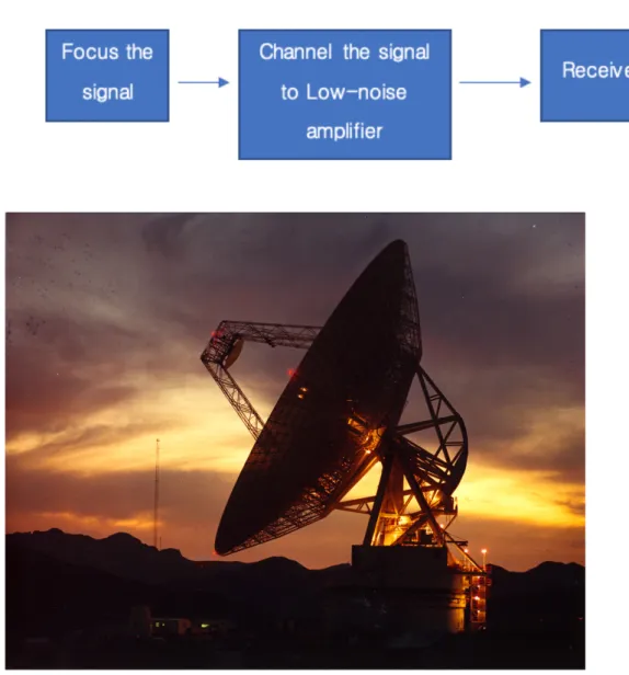
Figure 2.7: RF communications block diagram. Credit: ESA

2.5.2 Ground segment

The communications with the spacecraft have been performed through the ESA 35 m deep space ground station located in Cebreros, near Madrid in Spain (DSA2). The observations carried out with VeRa required additional support which came from the 35m New Norcia ground station (DSA1). In addition, during critical periods, also the NASA Deep Space Network (DSN) participated in the mission. In the frame of this work the data analyzed is the one received from the DSN.

(39)

2.5.2.1 The Deep Space Network

The DSN consists of three facilities spaced equidistant from each other – approx-imately 120 degrees apart in longitude – around the world. These sites are at Goldstone, near Barstow, California; near Madrid, Spain; and near Canberra, Australia. The strategic placement of these sites permits constant communication with spacecraft as our planet rotates – before a distant spacecraft sinks below the horizon at one DSN site, another site can pick up the signal and carry on commu-nicating, see Figure 2.9. As well known, the Deep Space Network is fundamental for communicating with deep space missions, however this Network is also able to generate accurate radio science data observables. From the general point of view, the parabolic surface of the antenna focuses the radio-frequency energy, coming from the spacecraft, onto a subreflector, which is adjusted in position to optimize the transfer of energy to the other systems within the complex. Firstly, it is in-teresting in understanding the two methods to keep the antennas pointed at the spacecraft. The first method, is the closed loop “CONSCAN” where the acquired signal is conically scanned by the antenna. Then the feedback from the closed loop receiver provides information comparable to the scan pattern of the received signal, and compensates to point the scan center at the apparent direction of the spacecraft signal. However, in case of high signal dynamics or low received signal levels (what usually happens in occultation experiments) the CONSCAN cannot be used and the antenna is “blind pointed” by using predicted ephemeris from the spacecraft navigators which are transformed into antenna’s coordinates.

Even for the reception of the signal in the Deep Space Network there are two di↵erent methods: the first one, and not used in radio occultations experiments, is the closed-loop reception which provides, through the feedback, a rapid acquisition of the signal and the telemetry lockup. However, this method requires some time to lock-up the signal (especially during the egress of occultations when the signal from the spacecraft is lower) and could lead to loss of crucial data. That is the reason why the open-loop reception method is adopted for these experiments and so in this research, which have been conducted through data received in open-loop. The open-loop receivers rely on frequency predicts to remain tuned to the incoming signal. To conclude, the signal is downconverted from RF to IF and then from IF to VF which is in the end the type of data processed for the experiments [2].

(40)

Figure 2.8: NASA Deep Space Network Goldstone Complex, California. Credit: NASA

(41)

(42)

(43)

Chapter 3

Radio Occultations

This chapter will give a description of the main theoretical topics needed, within the frame of this work, for conducting and studying radio science experiments, as well as the mathematical model and the understanding needed to describe the results obtained will be showed. In particular, Section 3.1 will cover a general background on the radio science experiments. Section 3.2 will be focused on the signal processing, with a description of how to obtain the reconstructed frequency residuals starting from the recorded radio signal in the time domain. To conclude, Section 3.3 will go into the details of the mathematical model employed in radio science investigations, to convert the reconstructed frequency residuals into the relevant atmospheric parameters of the target.

3.1 Theoretical background

The Radio occultation investigations are remote sensing techniques, which employ a radio signal between a transmitter and a receiver to measure physical properties of a target, as a planetary body. These have been commonplace on planetary science flyby and orbital missions since Mariner 4 reached Mars in 1965 [11], with dozens of spacecrafts performing radio occultations at many planets, satellites, and a comet [23]. The first studies and theories, as well as the mathematical models needed for these radio science investigations, dates back in the 60’s ( the first radio occultation experiment was done by Mariner IV on the 15th July 1965) when Phin-ney [18] and Eshleman [5] presented the first studies. Then, lot of research have been done on these theories from Eshleman, Fjeldbo, Kliore, Anderson, Phinney

(44)

Radio Occultations

etc. From the general point of view, the atmospheric radio occultation investiga-tions, which are the focus of this work, rely on the detection of a change in a radio signal as it passes through the atmosphere of a solar system object. This is due to the fact that when an electromagnetic radiation passes through the atmosphere, it is refracted, as can be seen from Figure 3.1 .

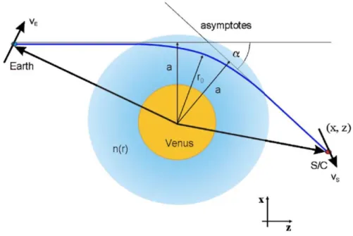
Figure 3.1: Ray bending in the atmosphere. r0 = ray path closest approach distance;

↵ = deflection angle; a = impact parameter; n=index of refraction. [8]

The refraction of the radio signal in the neutral gas and ionospheric plasma around the target object modifies the frequency of the radio signal, which is, in the end, di↵erent with respect to what expected by the receiver if no occultation would have occurred. In this way is possible to evaluate the frequency residuals, which represent the di↵erence between the modified frequency during occultation, and the expected direct frequency without refraction and occultation. By analyzing and processing the frequency residuals during a radio occultation investigation, the physical properties of the target object can be obtained. For example, vertical profiles of the electron density of ionospheric plasma, number density of neutral gas, pressure, temperature and mass density of the planetary body can be ob-tained, starting from the frequency residuals defined before. To do so, a detailed

(45)

Radio Occultations

knowledge of the positions and velocities of the transmitter, receiver and target, as a function of time, is required for the success of the radio occultation investi-gation. Furthermore, since these positions and velocities are related to times, the knowledge and accuracy of the time evaluation is crucial for the success of the experiments, as well.

From the geometrical point of view, an occultation experiment can be classified as:

• Ingress / egress occultation;

• Grazing occultation.

The ingress/egress experiment is the most common to analyze, easier with respect to the grazing, and is made by two di↵erent and separate phases, see Figure 3.2. The ingress phase happens when the spacecraft is getting close to the planet, then its signal starts traveling through the planet’s atmosphere so that it is refracted. The spacecraft then disappears behind the planet as seen by the ground station, which is not able to receive the signal anymore. On the other hand, the egress phase is defined when the spacecraft reappear from behind the planet, so that the ground station is able to receive its signal, again. Here another refraction takes place as the spacecraft’s signal pass through the planet’s atmosphere. In the end, in each phase is possible to obtain scientific data getting the atmospheric properties of the target. A plot of the typical signal recorded by the ground station during an ingress/egress occultation experiment is reported in Figure 3.4a.

(46)

Radio Occultations

Figure 3.2: Ingress (left) and Egress (right). In this case a star occulted by Venus is represented, but the geometry of the occultation is the same for the spacecrafts, too.

Credits: https://www.skyandtelescope.com/observing/venus-occults-a-star/

Figure 3.3: Grazing occultation of Aldebaran star by the Moon.

As can be seen, the star (or spacecraft) never disappear, it travels slightly above (or under) the planet, so that the signal is always recordable, but weaker due to atmospheric losses.

Credits: http://astroguyz.com/2017/03/31/astro-vid-of-the-week-an-amazing-grazing-occultation/

(47)

Radio Occultations

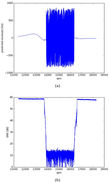
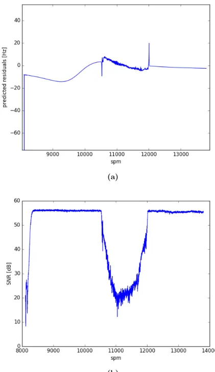
(a)

(b)

Figure 3.4: Ingress/egress typical processed signal of the occultation occurred the 17th _{February 2014, recorded by JPL. a) Second past midnight (spm)}

vs residual frequency: in the middle region the residuals are high and the signal is dominated by noise because the spacecraft was occulted by Venus. b) spm vs Signal to Noise Ratio (SNR), in the middle the noise is dominant, so the SNR decreases.

(48)

Radio Occultations

Regarding the Grazing, the spacecraft never disappears behind the planet, so there is not a clear ingress and egress phase, see Figure 3.3. Usually, it travels above or under the planet, always visible by the ground stations, but at some point, the signal becomes weaker as it starts passing through the atmosphere of the planet, which cause an amplitude loss. A plot of the typical signal recorded by the ground station during a grazing occultation experiment is reported in Figure 3.22a.

The Section 3.3 will show the details of the mathematical formulation, presented by Withers (2014) [24] , needed to solve the radio occultation problem. In particular, Withers summarize the theories developed in the 60’s, optimizing the mathematic formulation of the problem with the goal of developing an algorithm capable to solve the radio occultation problems. The MATLAB algorithm developed in the frame of this investigation follows the guidelines of Withers (2014) [24], as well.

(49)

Radio Occultations

(a)

(b)

Figure 3.5: Grazing processed signal of the occultation occurred the 19th March

2014, recorded by JPL. a) Second past midnight (spm) vs residual frequency.

b) spm vs SNR: note that with respect to the ingress/egress occultation (Figure 3.4a) the SNR does not decrease as in the previous case, because the spacecraft is not occulted by the planet. The decrease of the SNR is caused by the atmosphere of the planet.

(50)

Radio Occultations

3.2 Observables

The state of the spacecraft, or observables, is measured on ground, by collecting the scalar quantities information from the onboard tracking systems. This work has been focused on the two main radiometric measurements: one-way range and one-way range rate, which have been carried out by the radio science instruments on board the VEX and MGS spacecrafts.

3.2.1 One-way range

The range measures the linear distance between the spacecraft and the Earth. The idealized linear distance between the two bodies can be defined as:

⇢ =p[(r rI)· (r rI)] (3.1)

where r is the position vector of the ground station, while rI is the position vector

of the spacecraft, both of them evaluated with respect to the origin of the reference coordinate system (in this case Earth-centered one). The range, is a function of the time, in particular of the specific instant of time at which the observable is measured, so to be precise rI = rI(t light time) and r = r(t light time).

In the ideal case, the true range would be the same as the observed range, however due to instrumental limitations, medium propagation, Earth’s atmosphere and the dynamics when the spacecraft approaches a planet, the observed range is di↵erent with respect to the real and actual radial distance, so that the observed range can be defined as:

⇢obs = ⇢ + ✏ (3.2)

where ✏ is the term which considers all the errors.

From the practical point of view, this radiometric measurement can be obtained through the measure of the one-way time of flight of a radio signal between the two bodies. In the one-way range, the signal is generated by the spacecraft transponder at time tT and received by the ground station at time tR, the so called downlink.

So the one-way range is [16]:

(51)

Radio Occultations

where c is the speed of light, and ✏ as before takes into account all the errors which are described in the described la

3.2.2 One-way range rate

Range-rate measurements are related to the rate of change, with respect to time, of the radial distance between the spacecraft and the ground station. The range-rate, from the mathematical point of view can be obtained by di↵erentiating in time the Equation 3.1. Or from the practical point of view could be seen as:

˙⇢obs = ˙⇢ + ✏ (3.4)

where ✏ represents the errors as before.

Furthermore, with some mathematical definitions and manipulations (for the de-tails see [16], Section 3.2.2), the range-rate could be related to the recordings of the Doppler shift of a radio signal, which has been the core of this work:

fT fR = f = fT

˙⇢

c (3.5)

where fT is the transmitted frequency from the spacecraft, while fR is the received

(52)

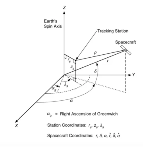
Radio Occultations

Figure 3.6: Range definition and reference coordinate systems for the spacecraft and ground station. Credit: NASA

3.3 Signal Processing

The spacecraft’s signals used within the framework of this research have been recorded by the NASA Deep Space Network (DSN). As explained in Subsection 2.5.2.1, in order to eliminate the loss of data due to closed-loop receiver lock-up time at the occultation egress, an open-loop reception method is the one adopted. The signal recorded from the ground stations, must be processed in order to get the frequency residuals, which are the inputs of the MATLAB algorithm devel-oped. From the general point of view, the signal must be converted from the time domain to the frequency domain, then after some manipulations and evaluations, the frequency residuals can be computed. A detailed explanation of all the steps covered within the Signal Processing is provided in the next subsections.

(53)

Radio Occultations

3.3.1 Data information

The Venus occultation data selected comes from Venus Express, which are one-way link, single frequency X-band, from 2014. On the other hand, for Mars, the occultation data is from Mars Global Surveyor, one-way, single frequency X -band. Before discussing the steps of the signal processing, is interesting to show the information of the data collected, see Figure 3.7.

Figure 3.7: Information about the occultation data 248V EOE2014044 0325N N N X43RD.1B1 occurred on the13th February 2014.

Each datafile is classified with its Start Time and End Time, in which the Year and the Day of the year (DOY) are also reported. For example, the DOY 044 is referred to the 13th _{of February 2014. The Spacecraft No. 248 stands for the ID}

number of the spacecraft, in this case Venus Express; the Sample Rate is referred to the sampling of the signal, which is the reduction of a continuous-time signal to a discrete-time signal. The sampling frequency or sampling rate, fs, is the average

number of samples obtained in one second (samples per second), thus fs = 1/T,

(54)

Radio Occultations

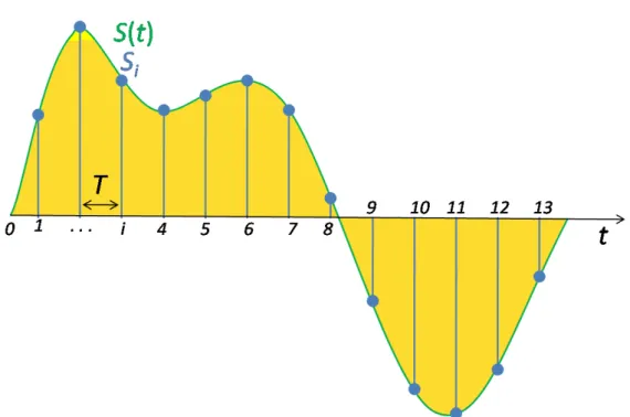
Figure 3.8: Signal sampling representation. The continuous signal

(green colored line) is replaced by the discrete samples (blue vertical lines). Credit: https://en.m.wikipedia.org

(55)

Radio Occultations

Another important information is the Tracking Mode, which, as explained in Sec-tion 2.5.1, for radio science experiments (especially egress occultaSec-tions) is usually set as one-way link. This is the reason why in the signal information of Figure 3.7 only the Downlink Band (for this data the X band, which refers to a frequency of 8.4 GHz) is reported. The ground stations, in fact, is not sending any signal to the spacecraft, and the whole experiment relies on the frequency sent by the space-craft and so by the efficiency of the Ultra Stable Oscillator onboard the spacespace-craft, which provided a high-quality onboard reference frequency source. The Figure 3.9 shows the outline of the work needed to process the data, which will be explained in details, step by step.

3.3.2 Signal (time domain)

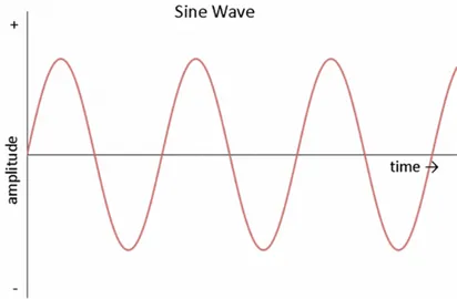
The time-domain carrier signal recorded by the DSN can be defined as a sine wave or sinusoid, as Equation 3.6, and a typical plot is reported in Figure 3.10.

A(t) = Asin(2⇡f t) + n(t) (3.6)

Figure 3.10: Sine wave. Credit: https://www.investopedia.com/terms/s/sinewave.asp

This signal is typically represented in a plot with the time in the x-axis and the am-plitude in the y-axis. However, since the goal of the Signal Processing is to obtain the reconstructed frequency residuals of the signal received from the spacecraft, as a first step the signal must be transformed in the frequency domain. Then, after

(56)

Radio Occultations

some manipulations the frequency residuals will be analyzed, through the Abel transform, and will unveil the atmospheric properties of the target. So, the first task of this work has been to process the VEX data, starting from a time-domain signal and converting it into the frequency-domain. The tool which permits to do this conversion is the Fourier Transform, which is addressed in the next subsection.

3.3.3 Fourier transform

The Fourier transform decomposes a function of time into its constituent frequen-cies. The Fourier transform of a function in the time-domain is itself a complex-valued of frequency, whose magnitude (the modulus) represents the amount of that frequency present in the original function, and whose argument is the phase o↵set of the basic sinusoid in that frequency.

The Fourier transform of a function f can be expressed as F by:

F_{{g(t)} = G(f) =} Z ₁

1

g(t)e 2⇡if tdt (3.7)

As a result, G(f ) gives how much power g(t) contains at the frequency f . G(f ) is often called the spectrum of g. A simple example to understand how the Fourier transform works is reported here, where the box function of Figure 3.11 is analyzed.

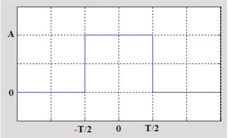
Figure 3.11: Box function (time domain).

(57)

Radio Occultations

By evaluating the Fourier Transform on the box function, the result is:

F{g(t)} = G(f) = Z 1 1 g(t)e 2⇡if tdt = Z T /2 T /2 Ae 2⇡if t_{dt =} A 2⇡if " e 2⇡if t T /2 T /2 # = A 2⇡if ⇥ e ⇡if T e⇡if T⇤= AT ⇡f T  e⇡if T _e ⇡if T 2i = AT ⇡f Tsin(⇡f T ) = AT [sinc(f t)] (3.8)

The plot of the Fourier Transform of the box function, in the frequency-domain, is reported in Figure 3.12.

Figure 3.12: Spectrum of the box function.

Credit: http://www.thefouriertransform.com

The Fourier Transform permits to convert the signal from the time domain (Fig-ure 3.11), to the frequency domain, as in Fig(Fig-ure 3.12. Furthermore, the Fourier Transform is extremely useful to highlight the component frequencies of the signal recorded, which is the first step to get the frequency residuals.

(58)

Radio Occultations

3.3.4 Signal (frequency domain)

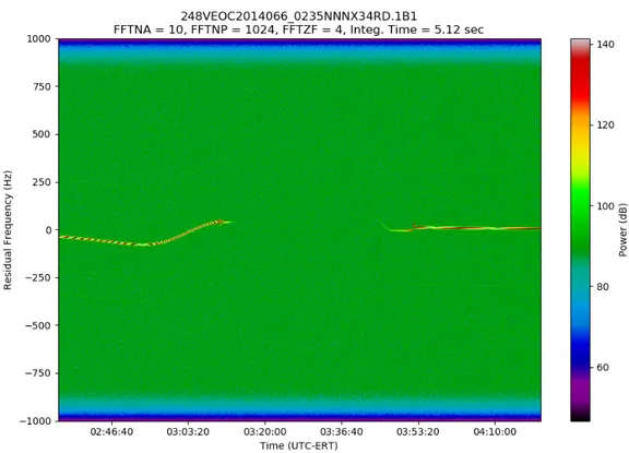
From the practical point of view, this process can be observed by running a JPL spectrogram tool, which first of all highlight the power of the recorded signal during the experiment, see Figure 3.13. Then, for each selected point the tool runs a FFT algorithm in order to show the main component frequency of the signal at the instant of time selected, see Figures 3.14 ; 3.15. By studying the signal in the frequency-domain, as for example the one reported in Figure 3.14, which is related to one of the VEX data recorded by the Deep Space Network of NASA and managed by JPL, is possible to understand which is the main frequency, also called component frequency, of the recorded signal at a certain instant of time.

In Figure 3.14 a spectrum of the signal recorded at the Deep Space Station 43 has been computed through a Jet Propulsion Laboratory tool, which evaluate the predicted residual frequencies of the recorded signal and its power. To do so, it runs a Fast Fourier Transform algorithm, also called FFT, which computes a Discrete Fourier Transform (DFT) on the signal. The residual frequency, also called predicted frequency residual, showed in the plot are the di↵erence between the observed frequency (skyfrequency) and the predicted frequency. Thanks to this tool is possible to obtain the main frequency (or main component frequency) of the signal at a certain instant of time (in this case at 03:02:48 of the 7th _March

2014). The component frequency is the one characterized by the highest power and is collected, and used, for the next steps of the signal processing. All the others low-power frequencies showed in the plot represent the noise present in the recorded signal. This process can be done with di↵erent accuracies depending on how much samples of the signal are being considered. Within this work the signals are processed with a time-step of 0.25 seconds or 0.5 seconds (so each 0.25 or 0.5 seconds of the time-domain signal a reference frequency will be collected), which represents a good trade-o↵ between the number of points analyzed and the thermal noise. In fact, by decreasing the integration time, the thermal noise introduced by the FFT increases, so the quality of the frequency residuals decreases, leading to a higher uncertainty in the results. A detailed explanation of the selection of the time-step and the noise related to it will be provided in the Section 4.3.

To conclude this subsection, it is interesting to show how the spectrum of the received signal looks like when the spacecraft is occulted by the planet, see Figure

(59)

Radio Occultations

Figure 3.13: Spectrogram of the VEX radio signal recorded by the DSN on the ingress/egress occultation of the 7th March 2014.