6 - Results and Analysis of the First Scenario vs the Second Scenario

(1)

6 - Results and Analysis of the First Scenario vs the

Second Scenario

6.1 – Overview

The objective of this chapter is to compare the first scenario, the one without any QoS (all

traffic is treated as best effort), with the second scenario, where is applied a DiffServ

treatment to the flows together with Constraint based Routing to obtain a dynamic traffic

engineering. The comparison on the first part of this chapter regards mainly the

improvement on the UDP traffic, while in the second part the attentio n is focused on the

improvements brought to the TCP traffic.

In section 6.2 three simulations will be analyzed, overloading at first the Gold UDP traffic,

then the Silver UDP and at last both Gold UDP and Silver UDP traffic. In order to show, as

explained on chapter 5, that the excess traffic in one class does not damage the others. It

will be also shown that the network provides a larger throughput thanks to the use of traffic

engineering that will make a better traffic distribution through the available paths.

In section 6.3 many simulations will be used to analyze the TCP traffic pattern through a

series of graphs.

In all the simulations made with the second scenario the objectives determined by the SLA

(2)

6.2 – UDP Varying

6.2.1 – Simulation 1 - Gold class overloaded, Silver class underloaded.

In this section, a first simulation is presented. In this case, the Gold class is overloaded and

the Silver class is under loaded.

The UDP traffic pattern generated as described in sectio n 5.4 is presented on Table 1. The

average rate is 383 Kbit/s for Gold traffic, 50 Kbit/s for Silver and 22 Kbit/s for Bronze.

The total rate is 4100 Kbit/s.

As regards the first scenario, there is no admission control, so all the traffic is treated as

best-effort (here the denomination of Gold, Silver and Bronze is just formal) following the

shortest path from the source to the destination. Obtaining a total rate (all best-effort) of

4100 Kbit/s with an average rate (27 aggregated flows because the traffic is full duplex,

but in the tables is represented just the traffic in one direction, the traffic in the other

direction is exactly the same) around 152 Kbit/s per AgF (Aggregated Flow).

Traffic Rate Full Duplex (CBR Sources) Gold Traffic Kbit/sec

From / To Node 17 Node 16 Node 15 Total Rate

Node 14 400 400 300 1100

Node 13 450 450 450 1350

Node 12 300 400 300 1000

Total Rate 1150 1250 1050 3450

Silver Traffic Kbit/sec

Node 14 100 100 50 250

Node 13 50 0 100 150

Node 12 0 0 50 50

Total Rate 150 100 200 450

(3)

Node 14 50 0 50 100

Node 13 50 0 0 50

Node 12 0 0 50 50

Total Rate 100 0 100 200

Tab 6.1 – Traffic generated

As regards the second scenario, the Gold traffic is over the reservation, while the Silver

one is under the Silver reservation; the admission control reclassifies the exceeding Gold

traffic to Silver and Bronze (if no silver bandwidth is available), as can be seen in Table 2.

For example, the AgF between nodes 13 and 17 is reclassified to both lower classes, at

first from Gold to Silver till filling the bandwidth availability in that class, then putting the

exceeding bandwidth left into the Bronze class.

Node 14 300 300 300 900

Node 13 300 300 300 900

Node 12 300 300 300 900

Total Rate 900 900 900 2700

Node 14 150 150 50 350

Node 13 150 150 150 450

Node 12 0 100 50 150

Total Rate 300 400 250 950

Bronze Traffic Kbit/sec

Node 14 100 50 50 200

Node 13 100 0 100 200

Node 12 0 0 50 50

Total Rate 200 50 200 450

(4)

We obtain an average rate of 300 Kbit/s for Gold, 106 Kbit/s for Silver and 50 Kbit/s for

Bronze. The total rate is 4100 Kbit/s.

6.2.1.1 - UDP Packet Loss

Percentage of Packets Lost for each service class

Gold Silver Bronze

39% 52% 49%

Percentage of Packets Received for each service class

Gold Silver Bronze

61% 48% 51%

Tab 6.3 – Packet Loss Scenario 1

Goodput Gold 2104,5 Kbit/s

Goodput Silver Total rate

216 Kbit/s 2422,5 Kbit/s

Goodput Bronze 102 Kbit/s

Tab 6.4 – Goodput Scenario 1

Percentage of Packets Lost for each service class Gold Silver Bronze

0% 0% 15%

Percentage of Packets Received for each service class Gold Silver Bronze

100% 100% 85%

Goodput Gold 2700 Kbit/s

Goodput Bronze 382,5 Kbit/s

The results, regarding the improvement in the number of packets lost, are considerably

good. A fundamental result, essential in order to speak about quality of service, is to have

no packet loss for the Gold and Silver class. This was achieved in the second scenario and

can be easily understood as the reservations for the Gold and Silver traffic classes are

never exceeded. Since each class has priority for using its reserved resources, an overload

(5)

improvement for the Bronze packet loss, that is more than halved, passing from 49% of

packets lost to 15%. This results from the traffic engineering that provides a better traffic

distribution in the network.

Tables 4 and 6 report the Goodput, that is the effective rate received at the last router of

the MPLS domain for each traffic class, corresponding to the effective end to end rate the

applications get from the network. It can be noticed that the total Goodput is almost

doubled in the second scenario. This also results from the traffic engineering that takes

advantage of the redundant paths in the network to successfully transport more traffic.

6.2.1.2 - UDP Delay

Average delay ms

Gold Flows Silver Flows Bronze Flows

90,80 83,50 81,30

Standard Deviation ms

46,90 37 35,05

Tab 6.7 – UDP Delay scenario1

Average delay ms

32,75 38,81 55,73

10,08 7,00 24,97

Tab 6.8 - UDP Delay scenario2

To limit the delay is fundamental in a phone call. A high value for this parameter could

make the full-duplex communication difficult.

In the second scenario there is a great improvement for the delay. The average delay is

quite one third for the Gold class, while is more than halved for the Silver class, and quite

halved for the best effort traffic. As regards the standard deviation, we can see that using

MPLS, the differences among the various flows are not high, because there are lower

(6)

The use of different traffic classes with admission control to limit the load in each class

can provide low delay values for the important traffic classes. The traffic engineering also

improves the overall results in this case.

6.2.1.3 - UDP Jitter

Average jitter ms

2,11 4,84 4,76

1,48 2,85 2,90

Tab 6.9 – UDP Jitter Scenario 1

Average jitter ms

2,21 3,53 13,58

0,66 2,04 9,89

As we are treating phone calls, it makes sense to look at the jitter as an important

parameter to measure the level of QoS obtained. A bad value for the jitter can degrade a

lot a conversation.

It may seem that the improvements brought by the use of MPLS are not extendible to the

jitter too. But, even if the results obtained in the first scenario are good, it makes sense to

speak about this parameter only in the second one. This happens because in the first

scenario there are too many packets lost to speak about the jitter.

6.2.1.4 – TCP Flows Rate

Total average rate Kbit/s Total rate Kbit/s

Gold 8,41 530

Silver 8,80 342

Bronze 5,69 512

Total 1384

Tab 6.11 – TCP average rate Scenario 1

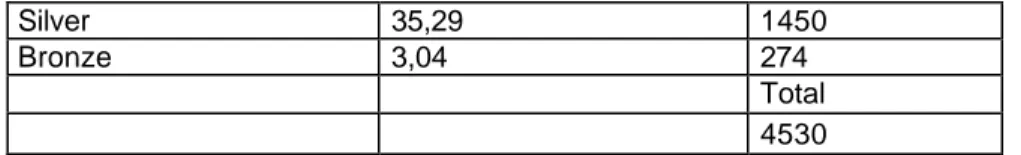
Total average rate Kbit/s Total rate Kbit/s

(7)

Silver 35,29 1450

Bronze 3,04 274

Total 4530

Tab 6.12 – TCP average rate Scenario 2

The analysis of the TCP flows rate is made in this section (6.2) related to UDP varying

just to give a simple idea of the advantages obtained and to take into account the total

average rate, as this parameter will be useful for a final analysis of this section.

The improvements brought by the second scenario are really high even in this case. The

total rate obtained by the Gold TCP traffic is almost six times the one obtained in the first

scenario. The Silver total rate is, more or less, five times bigger. The only thing that

appears worse is the Bronze traffic, but we do not care very much about that, because it is

best effort traffic.

6.2.2 – Simulation 2 - Gold class under loaded, Silver class overloaded.

In this subsection, a second simulation is presented. In this case, the Gold class is under

loaded and the Silver class is overloaded, just opposite to the situation of the first

simulation in the previous subsection.

Table 13 presents the UDP traffic generated as described in section 5.4. The average rate

is 161 Kbit/s for Gold traffic, 217 Kbit/s for Silver and 22 Kbit/s for Bronze. The total rate

(all best-effort) obtained is 3600 Kbit/s with an average (27 AgF ) value around 133 Kbit/s

per flow.

Node 14 0 250 150 400

Node 13 250 150 150 550

Node 12 200 250 50 500

(8)

Node 14 200 200 250 650

Node 13 250 200 200 650

Node 12 200 200 250 650

Total Rate 650 600 700 1950

Node 14 50 0 50 100

Node 13 50 0 0 50

Node 12 0 0 50 50

Total Rate 100 0 100 200

In the first scenario, there is no admission control, so all the traffic is treated as best-effort

following the shortest path.

In the second scenario, the Silver traffic is exceeding the reservations, while the Gold one

is under the reservation. The admission control puts the Silver exceeding traffic into the

Bronze, treating it as best effort traffic (Table 14).

We obtain an average rate of 161 Kbit/s for Gold, 150 Kbit/s for Silver and 89 Kbit/s for

Bronze.

Node 14 0 250 150 400

Node 13 250 150 150 550

Node 12 200 250 50 500

Total Rate 450 650 350 1450

Node 14 150 150 150 450

Node 13 150 150 150 450

Node 12 150 150 150 450

Total Rate 450 450 450 1350

(9)

Node 14 100 50 150 300

Node 13 200 50 50 300

Node 12 50 50 100 200

Total Rate 350 150 300 800

Tab 6.14 – Traffic effective with the second scenario

6.2.2.1 - UDP Packet Loss

Gold Silver Bronze

35% 42% 45%

Gold Silver Bronze

65% 58% 55%

Goodput Gold 942,5 Kbit/s

0% 0% 34%

100% 100% 66%

1350 Kbit/s 3328 Kbit/s

We have obtained no packet loss for the Gold and Silver class. There is also an

improvement for the Bronze class. These results are consistent with the conclusions of the

first simulation in the previous subsection, namely, the benefits of class protection and

(10)

As regards the Goodput, there is a good value, even if it is lover than the first simulation.

This happens because in the first simulation there is a potential maximum Goodput of

4100 Kbit/s, corresponding to the total traffic generated, while in this second simulation

the potential maximum Goodput is 3600 Kbit/s.

6.2.2.2 - UDP Delay

Average delay ms

99,85 90,84 92,93

32,09 28,25 26,91

Tab 6.19 – Delay Scenario 1

Average delay ms

30,0 37,9 52,2

8,6 6,9 30,8

Tab 6.20 – Delay Scenario 2

Also in this simulation, there is a great improvement for the delay. The average is around

one third for the Gold and Silver class, while is quite halved for best effort traffic. The

results obtained in this simulation are still very good as regards the standard deviation.

6.2.2.3 - UDP Jitter

Average jitter ms

2,2 4,04 9,15

1,19 3,81 12,05

Tab 6.21 – Jitter Scenario 1

Average jitter ms

1,00 3,38 7,39

0,71 1,62 10,22

(11)

In this second simulation, the improvements brought by the use of MPLS are extendible to

the jitter too. But, also here the results obtained in the first scenario are good but without

any effective meaning in the QoS mechanism as explained before.

6.2.2.4 - TCP Flows Rate

Total average rate Kbit/s total rate Kbit/s Gold 9,25 600 Silver 10,32 374 Bronze 9,50 855 Total 1829

Tab 6.23 – TCP Flows rate Scenario 1

Total average rate Kbit/s total rate Kbit/s

Gold 47,71 2793

Silver 37,08 1537

Bronze 3,74 337

Total 4667

Even in this case we have obtained really high improvements. The total rate obtained by

the Gold TCP traffic is almost four times the one obtained in the first scenario. The Silver

total rate is, more or less, five times bigger.

6.2.3 – Simulation 3 - Gold and Silver classes overloaded.

In this subsection, a third simulation is presented. In this case, both the Gold and Silver

classes are overloaded.

Table 25 presents the UDP traffic generated as described in section 5.4. The average rate

is 383 Kbit/s for Gold traffic, 189 Kbit/s for Silver and 22 Kbit/s for Bronze. The total rate

is 5350 Kbit/s, the highest among the three simulations. So, for the first scenario the

average value obtained for the 27 AgF is more or less 198,15 Kbit/s.

(12)

Node 14 400 400 300 1100

Node 13 450 450 450 1350

Node 12 300 400 300 1000

Total Rate 1150 1250 1050 3450

Node 14 150 150 150 450

Node 13 200 250 250 700

Node 12 200 200 150 550

Total Rate 550 600 550 1700

Node 14 50 0 50 100

Node 13 50 0 0 50

Node 12 0 0 50 50

Total Rate 100 0 100 200

In the second scenario, as both the Gold and the Silver traffic are exceeding the

reservations, the admission control declasses equally the excess Gold traffic and the

excess Silver traffic to Bronze. In this case there is no Silver bandwidth available to be

used. The resulting traffic pattern is presented in Table 14.

We obtain an average rate of 300 Kbit/s for Go ld, 150 Kbit/s for Silver and 144 Kbit/s for

Bronze.

Node 14 300 300 300 900

Node 13 300 300 300 900

Node 12 300 300 300 900

Total Rate 900 900 900 2700

Node 14 150 150 150 450

Node 13 150 150 150 450

Node 12 150 150 150 450

(13)

Node 14 150 100 50 300

Node 13 250 250 250 750

Node 12 50 150 50 250

Total Rate 450 500 350 1300

Tab 6.26 – Traffic effective with the second scenario

6.2.3.1 - UDP Packets Loss

Gold Silver Bronze

52% 56% 52%

Gold Silver Bronze

48% 44% 48%

Tab 6.27 – UDP Packet Loss Scenario 1

Tab 6.28 – UDP Goodput Scenario 1

0% 0% 50%

100% 100% 50%

Tab 6.29 - UDP Packet Loss Scenario 2

Tab 6.30 - UDP Goodput Scenario 2

In this simulation we have obtained the best results, reaching a value of 4700 Kbit/s on the

total Goodput, still having no packet loss for the first two classes. Also for the best effort

(14)

decreases to 50%, the value obtained for the Goodput is the highest of the three

simulations, reaching 650 Kbit/s.

6.2.3.2 - UDP Delay

Average delay ms

101,63 101,66 87,93

33,00 32,73 29,49

Tab 6.31 – UDP Delay Scenario 1

Average delay ms

32,8 39,4 56,8

9,9 7,5 27,4

Tab 6.32 – UDP Delay Scenario 2

There are very good results for the delay in this simulation too. The average Gold delay is

one third for the second scenario, and more than halved for the Silver delay, reaching good

results also for the Bronze. There are optimum results also as regards the standard

deviation.

6.2.3.3 - UDP Jitter

Average jitter ms

1,90 3,25 4,42

1,10 2,78 2,05

Average jitter ms

2,31 3,94 13,42

0,65 1,86 9,60

The jitter values are a little bit worse in the second scenario, but, as explained before, in

(15)

important is that the values obtained in the second simulation are largely more than

acceptable.

6.2.3.4 - TCP Flows Rate

Gold _4,64 ₃₀₄

Silver _4,01 ₁₃₁

Bronze _3,72 ₃₃₅

Total 770

Gold 45,15 2775

Silver 30,48 1315

Bronze _0,51 ₄₆

Total 4135

The TCP total rate growth is considerably high, the highest reached in the various

simulations. The values increase by more or less ten times for the first two classes, while

the best effort traffic is obviously reduced. The total rate for TCP+UDP is 8835 Kbit/s,

which is already near the maximum the network core can carry that is 9000 Kbit/s, so there

is almost no bandwidth left for Bronze traffic. This maximum value for the traffic the

network can carry is determined by the Max-Flow Min-Cut theorem [Tanenbaum, 81], that

states that:

The maximum flow between any two arbitrary nodes in any network cannot exceed

the capacity of the minimum cut separating those two nodes. Where a minimum cut

is defined as the set of links with minimum capacity whose removal disconnects

two nodes.

The maximum flow for the network core is the capacity of 9 core links (each 1000 Kbit/s),

(16)

Figure 6.1 – Minimum cut

6.3 – TCP Varying

In this set of simulations we will vary the TCP load, leaving the UDP fixed to heavily

loaded values. We want to show the better improvements brought by the second scenario

to the TCP flows.

Six groups of simulations will be analyzed, through the use of 12 graphs. In the first three

groups of simulations, the number of Silver TCP sources per AgF will be fixed

respectively to 1, 5 and 10, varying the number of Gold TCP sources. In the last three

groups of simulations, the number of Gold TCP sources per AgF will be fixed and the

number of Silver TCP sources varies.

The value represented in the graphs is the average rate per single class (Gold, Silver and

Bronze) flow, expressed in Kbit/s.

11

7

0

10

9

2

5

6

8

3

4

1

14

13

12

16

17

15

(17)

6.3.1 – Silver class TCP fixed, Gold class TCP varying.

The following graphs show the average rate per flow that the TCP flows in each class get

for a fixed number of Silver TCP flows and a varying number of Gold TCP flows. As can

be noticed by looking at the graphs, the results obtained by using the scenario 2 are

considerably better.

The rates that the flows get in the case of the fist scenario are totally irregular in graphs 1,

3 and 5, since all traffic is treated as best effort. On the other hand, in the second scenario

(graphs 2, 4 and 6), the rates are considerably regular and predictable for each class in all

the cases analyzed. This predictability is an essential and fundamental requisite to assure a

certain level of quality of service to a customer.

It can also be noticed a total independence among the classes in the second scenario, since

the treatment reserved to a class is independent from the traffic pattern in the other classes.

Scenario 1 - 1 Silver TCP sources

0,00 2,00 4,00 6,00 8,00 10,00 12,00 1 2 3 4 5 6 7 8 9 10 Gold TCP sources Rate Kbit/s Gold 1 Silver 1 Bronze 1 Graph 6.1

(18)

Scenario 2 - 1 Silver TCP sources 0,00 50,00 100,00 150,00 200,00 250,00 300,00 1 2 3 4 5 6 7 8 9 10 Gold TCP sources Rate Kbit/s Gold 2 Silver 2 Bronze 2 Graph 6.2

0,00 1,00 2,00 3,00 4,00 5,00 6,00 7,00 8,00 1 2 3 4 5 6 7 8 9 10 Gold TCP sources Rate Kbit/s Gold 1 Silver 1 Bronze 1 Graph 6.3

(19)

Scenario 2 - 5 Silver TCP sources 0,00 50,00 100,00 150,00 200,00 250,00 1 2 3 4 5 6 7 8 9 10 Gold TCP sources Rate Kbit/s Gold 2 Silver 2 Bronze 2 Graph 6.4

0,00 1,00 2,00 3,00 4,00 5,00 6,00 1 2 3 4 5 6 7 8 9 10 Gold TCP sources Rate Kbit/s Gold 1 Silver 1 Bronze 1 Graph 6.5

(20)

Scenario 2 - 10 Silver TCP sources 0,00 50,00 100,00 150,00 200,00 250,00 1 2 3 4 5 6 7 8 9 10 Gold TCP sources Rate Kbit/s Gold 2 Silver 2 Bronze 2 Graph 6.6

In the graphs 2, 4 and 6, we can see that the variation of the Gold TCP average rate is

always decreasing. This is obvious because the bandwidth reserved is the same

(300 Kbit/s) in all the simulations, while the number of sources sharing that bandwidth

increases linearly; this implies an average rate decreasing in an inverse proportion. The

TCP window adjustment mechanisms prevent a single TCP connection from using all the

available bandwidth.

The average value obtained by Silver TCP sources is more or less constant. It is near to the

reservation of 150 Kbit/s for graph 2 (all the bandwidth just for 1 Silver TCP source), 30

Kbit/s for graph 4 (bandwidth shared among 5 Silver TCP sources) and 15 Kbit/s graph 6

(21)

The best effort TCP traffic receives a low average value; this happens because the

bandwidth reserved to this class is only 50 Kbit/s and shared between TCP traffic and the

overloaded UDP one that takes great part of that bandwidth.

6.3.2 – Gold class TCP fixed, Silver class TCP varying

In this subsection the number of Gold sources per AgF will be fixed for each graph to 1, 5

and 10, while the number of Silver sources will vary along the graph.

Also in this second set of graphs it can be noticed the really great improvement brought by

the second scenario. The traffic pattern in the case of the fist scenario is totally irregular in

the graphs 7, 9 and 11 here too; while in the second scenario (graphs 8, 10 and 12) the

regularity and predictability is confirmed. It is confirmed also the independence among the

traffic classes.

Scenario 1 - 1 Gold TCP sources

0,00 1,00 2,00 3,00 4,00 5,00 6,00 7,00 8,00 1 2 3 4 5 6 7 8 9 1 0 Silver TCP sources Rate Kbit/s Gold 1 Silver 1 Bronze 1 Graph 6.7

(22)

Scenario 2 - 1 Gold TCP sources 0,00 50,00 100,00 150,00 200,00 250,00 300,00 1 2 3 4 5 6 7 8 9 10 Silver TCP sources Rate Kbit/s Gold 2 Silver 2 Bronze 2 Graph 6.8

0,00 1,00 2,00 3,00 4,00 5,00 6,00 1 2 3 4 5 6 7 8 9 10 Silver TCP sources Rate Kbit/s Gold 1 Silver 1 Bronze 1 Graph 6.9

(23)

Scenario 2 - 5 Gold TCP sources 0,00 20,00 40,00 60,00 80,00 100,00 120,00 140,00 1 2 3 4 5 6 7 8 9 10 Silver TCP sources Rate Kbit/s Gold 2 Silver 2 Bronze 2 Graph 6.10

0,00 1,00 2,00 3,00 4,00 5,00 6,00 7,00 1 2 3 4 5 6 7 8 9 10 Silver TCP sources Rate Kbit/s Gold 1 Silver 1 Bronze 1 Graph 6.11

(24)

Scenario 2 - 10 Gold TCP sources 0,00 20,00 40,00 60,00 80,00 100,00 120,00 140,00 1 2 3 4 5 6 7 8 9 10 Silver TCP sources Rate Kbit/s Gold 2 Silver 2 Bronze 2 Graph 6.12

Analyzing the graphs 8, 10 and 12, we can see that the behavior of the Gold and the Silver

TCP average rates are exactly the opposite than in the previous subsection. This happens

because now for the Silver traffic the bandwidth reserved is the same (150 Kbit/s) in all the

simulations, while the number of sources sharing that bandwidth increases linearly,

receiving an average rate per flow decreasing in an inverse proportion.

The average value obtained by a single Gold TCP source is more or less constant. It is near

250 Kbit/s for graph 8 (all the bandwidth is available for a single Gold TCP source, less

than the 300 Kbit/s reserved because of the TCP window management mechanisms),

60 Kbit/s for graph 10 (bandwidth shared among 5 Gold sources) and 30 Kbit/s for graph

12 (bandwidth shared among 10 Gold sources). To be precise, the last two values are a

little bit higher than 60 Kbit/s and 30 Kbit/s, reaching a value per AgF above the

(25)

signaling traffic is stolen by the Gold TCP traffic (the policing mechanism applied permits

to some AFs to steal the bandwidth unused by other AFs on the same path, if required).

Like in the previous subsection, the best effort TCP traffic receives a low average value for

the same reason.

One problem of the fixed reservations of scenario 2 can be observed in graphs 2, 10 and

12. If there is a small number of Silver sources and a large number of Gold sources, the

Silver sources can get a higher transmission rate than the Gold sources. This priority

inversion is undesirable since it is expected the Gold users will pay more than the Silver

users to get a better Quality of Service.

In the next chapter, a dynamic bandwidth assignment mechanisms will be shown that