Ottimizzazione di un processo di separazione magneto-gravimetrica in frazioni multiple. Optimization of a process for the Magnetic Density Separation into multiple fractions.

FACOLTÀ DI INGEGNERIA

CORSO DI LAUREA SPECIALISTICA IN

INGEGNERIA PER L’AMBIENTE E IL TERRITORIO

TESI DI LAUREA IN

VALORIZZAZIONE DELLE RISORSE PRIMARIE E SECONDARIE

OTTIMIZZAZIONE DI UN PROCESSO

DI SEPARAZIONE MAGNETO-GRAVIMETRICA

IN FRAZIONI MULTIPLE

OPTIMIZATION OF A PROCESS

FOR THE MAGNETIC DENSITY SEPARATION

INTO MULTIPLE FRACTIONS

Tesi di laurea di: Relatore:

Gabriella Meghini Prof. Ing. Alessandra Bonoli

Dipartimento di Ingegneria Chimica, Mineraria e delle Tecnologie Ambientali

Correlatore:

Dr. ir. Peter C. Rem Recycling Technology Delft University of Technology

Index

Abstract………...………... 1

Introduction ………... 6

1 Theory of magnetic separation …………... 7

1.1 Magnetism and innovation in magnetic separation ... 8

1.2 Fundamental quantities of magnetism and their units …... 10

1.2.1 Magnetic field and magnetization ... 10

1.2.2 Magnetic susceptibility and permeability ... 11

1.3 Magnetic properties of materials ...………... 12

1.4 Separation in magnetic fluids …..………... 14

1.5 Magnetic fluids: physical characteristics ... 15

1.5.1 Preparation of ferrofluids ………... 18

1.5.2 Viscosity of ferrofluids ………... 18

1.5.3 Stability of ferrofluids ... 18

1.5.4 The effect of temperature ...………... 19

1.5.5 Ferrofluid recovery and recycling …... 20

1.5.6 Ferrofluid applications ... 21

1.5.7 Safety data sheet of the ferrofluid used in this project ... 23

1.6 Magnetic fluids subjected to a magnetic field ... 24

1.6.1 Apparent density of a magnetic fluid ... 24

1.6.2 A particle suspended in a magnetic fluid …………...…... 25

1.6.3 The effect of the hydrodynamic drag ………... 27

1.6.4 Interaction of particles during separation ... 30

1.7 The Magnetic Density Separation (MDS) …..……...…... 31

1.8 The magnet ………...…………... 32

2 Magnetic density separator ... 33

2.1 Magnetic Density Separator: original layout ..…………... 34

2.2 First test: separating diamonds from gangue minerals ...……... 37

2.2.2 The fluid ………... 38

2.2.3 Time of separation ...………... 38

2.2.4 Flow measurements ………...………... 39

2.2.5 Results ………... 40

2.2.6 Problems found during experimentation ... 41

2.3 Rebuilding of the magnetic density separator ... 42

2.4 First layout ………... 42 2.4.1 Result………... 45 2.5 Second layout ………... 45 2.5.1 Results .………... 47 2.6 Third layout .………... 47 3 Experiments ………... 52

3.1 First test: preparation of the equipment ... 53

3.1.1 The magnetic fluid ………... 55

3.1.2 Sink-float tests …... 58

3.1.3 Time of separation ...………... 61

3.2 The experiments ………... 61

3.2.1 Wetting ……... 61

3.2.2 Frequency ……... 64

3.2.3 Interaction amongst particles of the same material ...70

3.2.4 Interaction amongst different materials ……... 72

3.2.5 Height of the gutter ……... 74

3.2.6 Final test ……... 76

3.3 Second test: preparation of the equipment ………... 77

3.3.1 The magnetic fluid... 81

3.3.2 Sink-float tests ………... 81 3.3.3 Time of separation ...………... 83 3.4 The experiments ………... 84 3.4.1 Test n.1 ……... 86 3.4.2 Test n.2 ……... 87 3.4.3 Test n.3... 87 3.4.4 Test n.4 ……... 88 3.4.5 Test n.5 …...…... 89

4 Conclusions and future developments ... 91

4.1 Conclusion ………...…... 92

4.2 Future developments ……...…………... 95

4.3 Applications ……….……….………... 99

Abstract

La separazione dei materiali in base alla densità è una tecnica universalmente riconosciuta: risulta essere uno dei più antichi metodi di lavorazione dei materiali. Immergendo un oggetto di densità ρ in un fluido con densità ρf, esso galleggerà se

ρ < ρf o affonderà se ρ > ρf. Con questa semplice strategia è possibile separare

materiali di diversa densità.

Il principio alla base della separazione magneto-gravimetrica prevede l’utilizzo di un fluido magnetico quale mezzo ideale di separazione. Questo fluido, costituito da una sospensione di particelle nanometriche di magnetite in acqua, ha una densità ρf relativamente bassa. In presenza di un campo magnetico, la sua densità

varia per il contributo della forza magnetica, il cui effetto si somma a quello della forza di gravità. Pertanto, per un fluido di magnetizzazione M, soggetto ad un gradiente magnetico B∇ , si ha:

g B M f a ∇ + =

ρ

ρ

Per un fluido magnetico immerso in un campo la cui induzione magnetica varia esponenzialmente con l’asse z, la densità apparente segue la legge:

( )

La densità del fluido sarà cioè maggiore negli strati più vicini al magnete, minore nelle zone più lontane. Pertanto un materiale immerso nel fluido tende a stazionare ad una determinata altezza (distanza dal magnete), in corrispondenza della quale la sua densità è uguale a quella del fluido.

Il Prof. Rem dell’Università di Delft (Paesi Bassi) ha progettato e brevettato un magnete che permette di ottenere un fluido magnetico con queste caratteristiche.

La separazione magneto-gravimetrica

Per poter sfruttare le proprietà dei fluidi ferromagnetici è stato messo a punto un separatore magneto-gravimetrico, grazie al quale è possibile separare diversi materiali in un solo processo. Il separatore è costituito da un canale vibrante in ottone posto sopra ad un magnete. Il fluido magnetico e i materiali da trattare sono inseriti all’interno del canale, dove avviene la separazione. I materiali vengono separati in base alla loro densità: ciascun materiale raggiunge una quota definita, punto di equilibrio tra la sua densità e quella del fluido.

La prima configurazione del separatore è stata usata per la separazione di diamanti da altri minerali. I risultati ottenuti sono stati incoraggianti.

Si è allora deciso di proseguire la sperimentazione, migliorando il separatore in alcuni punti e procedendo all’acquisto di nuove pompe.

Più in dettaglio, il processo di separazione può essere così riassunto:

• Il fluido magnetico viene fatto passare attraverso un laminatore, per evitare l’innesco di moti turbolenti che pregiudichino il processo. All’uscita del laminatore il fluido si mescola con i materiali destinati alla separazione (convogliati attraverso un ingresso preferenziale). L’insieme giunge quindi nell’area di separazione, soggetta al campo magnetico.

• Nell’area compresa tra il laminatore e gli scomparti di uscita avviene l’intero processo di separazione. In questa area il fluido magnetico è soggetto ad un campo magnetico non uniforme, pertanto il fluido ha una densità variabile a seconda della distanza dalla superficie del magnete. Ogni materiale immerso in questo fluido stazionerà ad un’altezza caratteristica, in funzione della propria densità.

• Un opportuno dispositivo sottopone il canale a vibrazione durante il processo

per evitare che i materiali si accumulino sul fondo o sulle pareti laterali del canale stesso.

• Alla fine del campo magnetico i materiali sono convogliati in cinque diversi scomparti (ognuno dei quali è costituito da tre lastre orizzontali che formano due settori di 10 mm di altezza). All’uscita di ciascun scomparto il fluido e il materiale vengono pompati verso un setaccio.

• Ogni setaccio provvede ad isolare la frazione di materiale dal fluido magnetico. Il materiale viene lavato e recuperato, mentre il fluido magnetico viene reintegrato nel processo mediante una pompa di ricircolo.

Esperimenti

Sono stati condotti diversi esperimenti al fine di valutare la bontà del processo di separazione e l’influenza di alcuni parametri sul processo stesso.

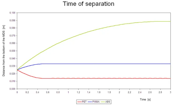
Nel primo esperimento sono state utilizzati tre tipi di plastica, le cui densità sono state misurate sperimentalmente con un picnometro a gas:

• PET: ρPET = 1351 kg/m3

• PMMA: ρPMMA = 1215 kg/m3

• ABS: ρABS = 1053 kg/m3

Per la separazione di questi materiali si è reso pertanto necessario un fluido magnetico che, sottoposto a un campo magnetico non omogeneo, variasse la propria densità all’interno dell’intervallo di valori 1050 - 1350 kg/m3. A tal fine, il fluido magnetico puro (M = 18000 A/m, ρf =1156 kg/m3) è stato diluito con 29

parti di acqua per raggiungere un intervallo di densità compatibile con i materiali. Successivamente è stata valutata l’altezza di galleggiamento di ciascun materiale, grazie ad un modello teorico sulla distribuzione della densità nel fluido e ad alcune prove pratiche. Ne è risultato che il PET affonda, di conseguenza dovrebbe essere raccolto nel primo scomparto, quello cioè più vicino alla superficie del magnete. L’ABS dovrebbe invece galleggiare sulla superficie del fluido, per essere raccolto nel quinto scomparto, cioè quello più lontano dal magnete. Infine il PMMA dovrebbe flottare ad un’altezza intermedia, per essere recuperato nel secondo e nel terzo scomparto.

Sono stati svolti numerosi test per determinare i parametri ottimali ai fini del processo. La miglior separazione è stata ottenuta con i seguenti accorgimenti:

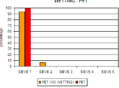
• I materiali sono stati precedentemente “bagnati” con un getto di vapore acqueo. In questo modo è stata scongiurata la formazione di bolle d’aria sulla superficie del campione, con inevitabile alterazione (diminuzione) della densità del materiale.

• La potenza delle pompe è stata regolata al 20% della loro capacità (pompe

sovradimensionate rispetto alle dimensioni del canale di separazione).

• Un alimentatore vibrante ha provveduto all’alimentazione dei materiali.

• Sono stati processati campioni con peso complessivo non superiore a 30 g per evitare problemi di intasamento delle connessioni tra le pompe e i tubi.

Il campione, costituito da PET, PMMA ed ABS, è stato inserito all’interno del sistema. Dopo alcuni secondi la separazione delle tre plastiche era già visibile. Tutto il PET è stato recuperato all’interno del primo setaccio (scomparto più basso, vicino alla superficie del magnete). Anche la separazione dell’ABS è avvenuta in modo ottimale, visto che tutto il materiale è stato raccolto nell’ultimo scomparto (il più lontano dal magnete), destinato alle frazioni più leggere. Il PMMA, la cui densità è intermedia, è stato raccolto in maggior parte nel terzo scomparto; la sua separazione non è stata ottimale perché piccole frazioni sono state raccolte sia nel secondo che nel quarto scomparto. Probabilmente questa frazione intermedia è maggiormente soggetta a fenomeni di perturbazione dovuti alla turbolenza nel flusso e/o all’interazione con i diversi materiali.

Altri test sono stati condotti utilizzando dei rifiuti da apparecchiature elettriche ed elettroniche (RAEE) forniti dall’azienda Axion Recycling Ltd, un insieme finemente macinato di plastiche (prevalentemente PVC), pietre, vetro e fili elettrici di rame.

L’obiettivo era quello di ottenere una frazione di rame più pura possibile.

L’elevata densità del rame lasciava supporre che questo venisse raccolto nella parte inferiore del separatore, e che tutti gli altri materiali, più leggeri, fossero destinati agli scomparti superiori.

Nonostante alcuni problemi di intasamento dei setacci, causati dalla forma e dalle dimensioni dei materiali trattati, i risultati ottenuti sono stati soddisfacenti. Il rame è stato recuperato nel primo setaccio, senza alcuna contaminazione da parte degli altri materiali, che si sono invece suddivisi in frazioni più leggere.

Conclusioni

La tecnologia di separazione magneto-gravimetrica è innovativa in quanto permette di separare materiali diversi in un solo passaggio. Si possono separare con risultati molto buoni sia materiali caratterizzati da densità simili a quella dell’acqua - plastica, sia materiali con densità decisamente superiori, come il rame, l’oro ed il platino.

Il processo potrà essere esteso a materiali di dimensioni maggiori utilizzando un canale più ampio.

Software di ausilio potranno invece essere impiegati per uno studio più approfondito del processo di separazione (simulazione del flusso, analisi dell’interazione tra i diversi materiali all’interno dell’area di separazione).

Le applicazioni di questa tecnologia ricoprono sia il campo dei rifiuti, dove il recupero dei materiali risulta economicamente vantaggioso ai fini industriali (si pensi ai metalli, che possono essere venduti alle filiere di riferimento), che quello dell’estrazione mineraria, dove si possono separare minerali e/o metalli preziosi da altri minerali o metalli.

Introduction

This project has been carried out at the Delft University of Technology, Section of Materials & Environment - Recycling Technology Laboratory.

In the first chapter the theory of the magnetic separation has been presented. The sink and float technique of gravity separation relies on selective levitation and sinking of materials based on their relative densities and that of the separating medium. In this study the application of magnetic fluids as a heavy medium has been investigated. The concept of separation of non-magnetic particles suspended in a magnetic fluid is based on the generalized Archimedes law whereby, in addition to the conventional force of gravity acting on the fluid, also a magnetically induced force acts on the fluids. This additional magnetic pull creates a magnetically induced buoyancy force on a particle immersed in the fluid. This buoyancy force can be controlled in a wide range of values and materials as dense as 20000 kg/m3 or higher can float in such a fluid.

In the second chapter some former tests with this technology have been shown and the re-building of the magnetic density separator has been described. A separator has been designed in order to separate multiple density fractions at once. The main part of the separator is a brass vibrating gutter. Fluid and non-ferrous materials are led into the gutter, straight into the magnetic field where the separation begins. At the end of the magnetic field the different density fractions are pumped towards a sieve. Here the materials are collected and the fluid is recovered and circulated.

In the third chapter some experiments have been performed and results have been shown. The tests have been carried out with different samples. Plastics as well as material derived from WEEE have been used. The separation of the plastics shows the whole potential of this process: they are recovered in different fractions on the grounds of their density. The separation of a sample coming from mixed materials derived from WEEE has been done in collaboration with Axion Recycling Ltd. A pure fraction of copper has been obtained.

In the last chapter the results have been discussed and new ideas for future developments have been given.

Chapter 1

1.1 Magnetism and innovation in magnetic

separation

Magnetic phenomena have been known and exploited for many centuries. The earliest experiences with magnetism involved magnetite, the only material that occurs naturally in a magnetic state. Thales of Miletus stated that the magnetic interaction between lodestone, or magnetite, and iron was known for at least as long ago as 600 B.C. That magnetite can induce iron to acquire attractive powers, or to become magnetic, was mentioned by Socrates. Permanent and induced magnetism, therefore, represents one of man’s earliest scientific discoveries. Practical significance of magnetic attraction as a precursory form of magnetic separation was recognized in 1792, when W. Fullarton obtained an English patent for separating iron ore by magnetic attraction. Since that time the science and engineering of magnetism and of magnetic separation have advanced rapidly and a large number of patents have been issued. While separation of inherently magnetic constituents was a natural early application of magnetism, Wetherill’s separator, devised in 1895, was an innovation of significant proportions. It demonstrated that it was possible to separate two components, both of which were commonly considered to be non-magnetic. In the ensuing time various types of disk, drum and roll dry magnetic separators were developed although the spectrum of minerals treatable by these machines was limited to rather coarse and moderately strongly magnetic materials. Since the end of the nineteenth century there has been a steady expansion of both the equipment available and the range of ores to which magnetic separation is applicable.

The development of permanent magnetic materials and improvement in their magnetic properties has been main drivers of innovation in magnetic separation. Figure 1.1 illustrates the history of improvement of the maximum energy product max of permanent magnets. Three innovation milestones can be identified in the graph. At the end of the nineteenth century very feeble steel based magnets were employed, while in the 1940s permanent magnets that were able to compete with electromagnets, were developed. Probably the most important innovation step was made in the late seventies of the last century when rare-earth magnets became available. These magnets allowed new solutions for challenges that were not possible or feasible with electromagnets.

Another significant driver of innovation in magnetic separation was the introduction of ferromagnetic bodies (such as balls, grooved plates or mesh) into the magnetic field of a separator. In 1937 Frantz developed a magnetic separator consisting of an iron-bound solenoid packed with ferromagnetic steel ribbons and this proved to be an important milestone in the development of the present high-intensity and high-gradient magnetic separators. This innovation extended the range of applicability of magnetic separation to many weakly magnetic and even to diamagnetic minerals of the micrometer size.

Although the significance of the discovery of superconductivity has been equated with the invention of the wheel, its importance for magnetic separation does not seem to represent a major breakthrough. The need for magnetic induction greater than 2 Tesla has never been convincingly demonstrated in matrix separators and the main advantage of superconducting magnets is, therefore, the reduced energy consumption and the possibility of generating a high magnetic force in large volumes, even without using matrices.

The concentration of various ferrous and non-ferrous minerals has been an important application of magnetic separation, as has the removal of low concentrations of magnetizable impurities from industrial minerals. In recent years, as a result of numerous economic, environmental and social challenges, the recycling of metals from industrial wastes and the concentration or removal of biological objects in medicine and biosciences have become important areas of

application of magnetic technology. Recent research and development of eddy-current separators, magnetic fluids and magnetic carriers illustrate the enormous effort that has been expended over the last twenty years in order to convert a wealth of novel ideas into workable techniques and introduce them into material manipulation operations.

1.2 Fundamental quantities of magnetism and

their units

In physics, a magnetic field is a vector field that permeates space and which can exert a magnetic force on moving electric charges and on magnetic dipoles (such as permanent magnets). When placed in a magnetic field, magnetic dipoles tend to align their axes to be parallel with the magnetic field. In addition, a changing magnetic field can induce an electric field. Magnetic fields surround and are created by electric currents, magnetic dipoles, and changing electric fields. Magnetic fields also have their own energy, with an energy density proportional to the square of the field intensity.

1.2.1 Magnetic field and magnetization

When a magnetic field is described, two different quantities, namely magnetic field strength H [A/m] and magnetic flux density (or magnetic induction) B [T], are employed.

H and B are both vector quantities having direction as well as magnitude. In vacuum B and H are not independent and are related by the equation:

0 B=

µ

µ is the magnetic permeability of vacuum.

In a magnetic material of magnetization M [A/m], the total magnetic induction becomes:

(

)

µ

Magnetization is defined as the total magnetic moment

µ

µ

In SI B is given by: J H B= + r r 0

µ

where J [T] is the magnetic polarization.

J and M are related by the following equation:

M J r r 0

µ

The magnetic induction thus includes contributions from the magnetization M, which is defined as the magnetic dipole moment of a body per unit volume, or polarization J defined by eq. (1.4).

1.2.2 Magnetic susceptibility and permeability

The magnetization of a material depends on the magnetic field acting on it. For many materials, M is proportional to H:

H k M r r = (1.5)

where k is the volume magnetic susceptibility, a property of the material. Since M and H have the same dimensions k is dimensionless.

We can combine eq. (1.5) with eq. (1.2) to get:

(

)

µ

µ

µ

µ

µ

(

)

The quantity

µ

whileµis called magnetic permeability and has a unit of H/m.

While eq. (1.2) is general, eqs. (1.6) and (1.7) are based on assumption that the material is both isotropic and linear. In other words, that M is proportional to H and in the same direction. This assumption is never completely true for ferromagnetic materials.

Either

µ

µ

Magnetic susceptibility can also be expressed with respect to the unit mass of material densityρ, and then

ρ

χ = k (1.8)

where χ [m3/kg] is the mass, or specific, magnetic susceptibility. Since a sample mass m is usually better known than its volume, mass magnetic susceptibility is very commonly employed. For the same reason the mass magnetization

σ

m

M µ

σ = thus M =ρσ (1.9)

1.3 Magnetic properties of materials

It has been stated at the outset that all materials display certain magnetic properties, regardless of their composition and state. According to their magnetic properties, materials can be divided into five basic groups: diamagnetic, paramagnetic, ferromagnetic, antiferromagnetic and ferrimagnetic. The last three groups have generally higher magnetic susceptibilities than the other groups and are frequently termed ”ferromagnetic” sensu lato (s.l.). This broad definition must be distinguished from one of its subdivisions, ferromagnetic sensu stricto (s.s.) as discussed below. The alignment of magnetic moments in each type of material is shown in Fig. 1.2.

Diamagnetism has its origin in the modification of the electron orbit magnetic moment by an external magnetic field. The currents thus induced give rise to an extra magnetic moment. However, according to Lenz’s law, the resulting magnetic moment is in the opposite direction to the field that has induced the current. Therefore, approaching a source of the magnetic field, a diamagnetic material is repelled from it. This effect is present in all materials, independently of temperature.

In paramagnetic materials the magnetic atoms or ions have permanent intrinsic magnetic moments and occur in low concentrations. Susceptibility arises from the competition between the aligning effect of the applied magnetic field and the randomizing effect of thermal vibrations. In zero applied magnetic field, the moments point in random directions. When a field is applied, a small magnetization develops, but the magnetic susceptibility is very small and is inversely proportional to the absolute temperature.

In ferromagnetic materials (s.s.) interaction between neighbouring atoms is strong so that the magnetic moments of all atoms are aligned parallel to each other against the randomizing force of thermal motion. The strong internal fields, which align the spins, are called molecular or Weiss fields. These fields are the result of a quantum mechanical process called exchange interaction. Weiss assumed that the molecular field is very large, its magnitude independent of external magnetic field, and its direction not fixed, but always parallel to the magnetization. The Weiss hypothesis predicts that a material can be spontaneously magnetized even in the absence of an applied magnetic field at temperatures below the Curie temperature, at which the thermal agitation overcomes the molecular field. This tendency aids the external field in producing saturation, i.e. complete alignment. There is an apparent contradiction between theory, which explains that magnetic materials are fully magnetized even in the absence of an external field, and practice, which generally shows that such materials exhibit no magnetization or magnetization much smaller than saturation. In fact, theory is correct at a microscopic level, but at a macroscopic scale the ferromagnetic body is subdivided into Weiss domains, each of which is spontaneously magnetized to saturation, but not in the same direction, by virtue of a strong exchange magnetic field. Inside a domain the magnetization is at a maximum (saturation), but as all domains compensate each other, on macroscale the mean magnetization is nil.

The value of the saturation magnetization varies with temperature, decreasing from a maximum value at T=0 K, becoming zero at the Curie temperature Tc.

Above Tc, the behaviour is similar to that of a paramagnetic material, with the

magnetization being proportional to the field and the susceptibility decreasing with increasing temperature.

In contrast to diamagnetic and paramagnetic materials, magnetization of ferromagnetic materials (s.l.) depends not only on the field strength, but also on the shape and the magnetic history of the sample. For instance, a ferromagnetic material can remain magnetized after removal of the external field.

Antiferromagnetic materials were originally thought of as a class of anomalous paramagnets, since they have small positive susceptibilities of similar magnitude to many materials of the latter class. However, their magnetic susceptibility does not increase steadily as the temperature decreases all the way to absolute zero. In a ferrimagnetic material magnetic moments are ordered regularly in an antiparallel sense, but the sum of the moments pointing in one direction exceeds those pointing in the opposite direction.

The magnetic properties of ferromagnets and ferrimagnets are generally similar: both exhibit saturation and their magnetization is much greater than that of other magnetic classes.

1.4 Separation in magnetic fluids

The sink and float technique of gravity separation relies on selective levitation and sinking of materials based on their relative densities and that of the separating medium.

In the mid sixties of the last century the application of magnetic fluids as a heavy medium, had been investigated, and it was established that by exposing a magnetic fluid to a non-homogeneous external magnetic field the fluid exhibited an apparent density exceeding densities obtainable with conventional heavy liquids.

The concept of separation of non-magnetic particles suspended in a magnetic fluid is based on the generalized Archimedes law whereby, in addition to the conventional force of gravity acting on the fluid, also a magnetically induced force acts on the fluids. This additional magnetic pull creates a magnetically

induced buoyancy force on a particle immersed in the fluid. This buoyancy force can be controlled in a wide range of values and materials as dense as 20000 kg/m3 or higher can float in such a fluid.

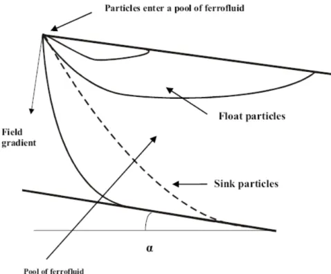
A schematic diagram of the process of separation in magnetic fluids is shown in Fig. 1.3. Permanent magnets or electromagnets are used to generate a non-homogeneous magnetic field in the separation gap. The desired pattern of the magnetic field and its gradient is achieved by shaping the pole tips. A separation chamber placed between the pole-pieces of the magnetic circuit is filled with a magnetic field.

1.5 Magnetic fluids: physical characteristics

Magnetic fluids can be divided into two broad classes, namely solutions of paramagnetic salts and ferrofluids.

Paramagnetic liquids, as the name indicates, are paramagnetic in their behaviour: their magnetization increases linearly with increasing magnetic field and their magnetic susceptibility is quite low, of the order of χ=5×10-7 m3/kg, and

independent. In addition to low magnetic susceptibility, some paramagnetic liquids tend to degrade in the presence of light; others tend to crystallize at lower temperatures, while others decompose at elevated temperatures. All such liquids are rather expensive and their recycling is essential, although not easy. The paramagnetic liquids have a high surface tension and do not wet the particles surface adequately.

A magnetic ferrofluid is a stable suspension of sub-domain magnetic particles, often magnetite, in a carrier fluid. Water, hydrocarbon and silicones are used as carrier liquids. The particles, which have an average size of 10 nm, are coated with a stabilizing dispersing agent, which prevents particle agglomeration, even when a strong magnetic field gradient is applied to the ferrofluid.

In the absence of an external magnetic field, the magnetic moments of individual particles are randomly distributed and the fluid has no net magnetization. When exposed to an external magnetic field, the ferrofluid becomes magnetized and reaches magnetic saturation at moderate magnetic fields. When the applied field is removed, the particles demagnetize rapidly and exhibit typical superparamagnetic behaviour characterized by the absence of coercivity and remanence. A typical magnetization curve of a ferrofluid is shown in Fig. 1.5. It can be seen that a high magnetic field is required to magnetically saturate a ferrofluid containing very small magnetite particles. This is a consequence of the difficulty in aligning the magnetic moments of very small particles.

Figure 1.4 - Magnetic particles, with clung surfactant molecules,

Although very small dimensions of magnetite particles improve the stability of a ferrofluid, the value of saturation magnetization decreases with decreasing particle size, as shown in Fig 1.6.

In weak magnetic fields the main contribution to magnetization is made by the larger particles which are more easily oriented by a magnetic field, whereas the approach to saturation is determined by fine particles, the orientation of which requires large fields.

Figure 1.6 - Saturation polarization of ferrofluids as a function of average particle size. Figure 1.5 - Magnetization curve of a ferrofluid with an average particle diameter 6 nm.

1.5.1 Preparation of ferrofluids

There are two basic methods of preparing a ferrofluid - size reduction and precipitation. Size reduction by wet grinding of ferrite in a ball mill, for a period of 1000 hours or longer, in the presence of a surfactant was developed to produce kerosene-based ferrofluids. Magnetite particles can also be prepared by precipitating the magnetite from a solution of ferric and ferrous ions using an excess of an alkali hydroxide solution. The particles are transferred from the aqueous phase to an organic phase containing a dispersion agent, such as, for instance, oleic acid. Subsequently, the particle dispersion in an organic phase is separated from the aqueous salt residue, filtered, and solvent adjusted to give the desired product concentration.

1.5.2 Viscosity of ferrofluids

The viscosity of a ferrofluid is one of the most important parameters that affect selectivity of separation in ferrofluid. In the absence of a magnetic field, the viscosity of a ferrofluid is greater than that of the carrier liquid as a result of the perturbation of the streamlines by suspended particles.

1.5.3 Stability of ferrofluids

The stability of ferrofluids in gravitational and magnetic fields is one of the fundamental parameters ensuring high selectivity of separation of materials in ferrofluids. Basic criteria for such stability can be obtained by investigating the balance of forces acting on the colloidal magnetic particles suspended in the carrying fluid. The relationship between the randomizing action of the thermal energy and the destabilizing effect of the gravitational field, surface forces, magnetic interaction between the particles and the non-homogeneous magnetic field, and between the particles themselves, determines the conditions under which a ferrofluid is stable.

It is fairly easy to show that while the force of gravity is of limited threat to the segregation of ferrofluids, the effect of magnetic agglomeration and of the field gradient can be eliminated only when the particle diameter is smaller than approximately 8 nm. However, molecular van der Waals forces that arise as a result of fluctuating electric dipole-dipole forces are always present in a colloidal

system. It transpires that infinite energy is required to separate a particle pair. Therefore, contact between individual particles must be prevented in order to obtain a stable colloidal suspension. Such a steric stabilization can be achieved by adding a chemical, for instance oleic acid, which can both adsorb on the surface of the particle and be solvated by the carrier liquid. This results in the formation of a bound liquid sheath around each particle. The most commonly used surfactant give a surface layer thickness of 2 nm to 3 nm.

The stability of kerosene-based ferrofluids used in ferrohydrostatic separators extend over periods as long as one year or longer. However, water-based ferrofluids usually contain particles somewhat larger than the particle in organic carriers. The destabilizing effect of magnetic agglomeration and the influence of the gravitational field might reduce the long-term stability that dispersants are not as effective as in organic carrier fluids.

1.5.4 The effect of temperature

A ferrofluid is, over a period of time, exposed to an increasing temperature as a result of the temperature increase in the windings of the electromagnet. The temperature increase results in an increase in the volume, and a decrease in the physical and apparent densities of the ferrofluid, at a constant concentration of magnetite. The change of the apparent density of a ferrofluid with temperature variation is illustrated in Fig. 1.7.

Figure 1.7 - The dependence of the apparent density of ferrofluid on temperature,

In addition to density, magnetic susceptibility also undergoes changes when the temperature of the fluid changes. It was observed that a temperature increase by 15°C results in the reduction of the magnetic susceptibility of the kerosene-based ferrofluid by 7% to 15%, depending upon the magnetic field strength to which the ferrofluid is exposed.

It is clear that temperature control of the ferrofluid and of the working environment in which a ferrohydrostatic separator operates, are essential for accurate performance of the equipment.

In this project the temperature will not affect the characteristic of the ferrofluid, because we are working on lab scale.

1.5.5 Ferrofluid recovery and recycling

In order to keep the running costs of ferrohydrostatic separators low, it is essential that the ferrofluid be recovered and recycled. At the same time, from the environmental point of view, it is imperative to remove tracers of ferrofluid from the products of separation.

A water-based ferrofluid adhering to the products of separation can be easily removed by washing the material with water. After the products of separation are washed with water, the diluted suspension is acidified to change the surfactant,

providing the secondary adsorption layer, to free acid. A thickener and a centrifugal separator can then be used to separate flocks from the excess water due to the washing process. The concentrated flocks thus obtained are re-dispersed as a concentrated ferrofluid by adding alkali and lost surfactant. The loss of ferrofluid in this process is claimed to be about 1% of the feed by weight. Diluted water-based ferrofluid can be re-concentrated also by ultrafiltration, a slow and potentially onerous process.

1.5.6 Ferrofluid applications

Ferrofluids are used to form liquid seals (ferrofluidic seals) around the spinning drive shafts in hard disks. The rotating shaft is surrounded by magnets. A small amount of ferrofluid, placed in the gap between the magnet and the shaft, will be held in place by its attraction to the magnet. The fluid of magnetic particles forms a barrier which prevents debris from entering the interior of the hard drive. Ferrofluids are also used in many high-frequency speaker drivers (tweeters) where they provide heat conduction from the voice coil to the surrounding assembly as well as mechanical damping to reduce undesired resonances. The ferrofluid is kept in place in the magnetic gap due to the strong magnetic field and is in contact with both the magnetic surfaces as well as the coil.

Mechanical engineering

Ferrofluids have friction-reducing capabilities. If applied to the surface of a strong enough magnet, such as one made of neodymium, it can cause the magnet to glide across smooth surfaces with minimal resistance.

Ferrari uses ferrofluid in some of their car models to improve the capabilities of the suspension. The suspension can instantly be stiffened or softened by an electromagnet, controlled by a computer.

Defense

The United States Air Force introduced a Radar Absorbent Material (RAM) paint made from both ferrofluidic and non-magnetic substances. By reducing the reflection of electromagnetic waves, this material helps to reduce the Radar Cross Section of aircraft.

Aerospace

NASA has experimented using ferrofluids in a closed loop as the basis for a spacecraft's attitude control system. A magnetic field is applied to a loop of ferrofluid to change the angular momentum and influence the rotation of the spacecraft.

Analytical Instrumentation

Ferrofluids have numerous optical applications due to their refractive properties; that is, each grain, a micromagnet, reflects light. These applications include measuring specific viscosity of a liquid placed between a polarizer and an analyzer, illuminated by a helium-neon laser.

Medicine

In medicine, a compatible ferrofluid can be used for cancer detection. There is also much experimentation with the use of ferrofluids to remove tumors. The ferrofluid would be forced into the tumor and then subjected to a quickly varying magnetic field. This would create friction, yielding heat, due to the movement of the ferrofluid inside the tumor which could destroy the tumor.

Heat transfer

An external magnetic field imposed on a ferrofluid with varying susceptibility, e.g., due to a temperature gradient, results in a non-uniform magnetic body force, which leads to a form of heat transfer called thermomagnetic convection. This form of heat transfer can be useful when conventional convection heat transfer is inadequate, e.g., in miniature microscale devices or under reduced gravity conditions.

Material Recycling

Ferrofluid has a unique property in that its apparent density can be increased by applying a magnetic field to the ferrofluid. This physical characteristic creates the ability to separate objects of different density through floatation or sinking. Ferrofluids have been used for years in material separation processes in the mining industries, although with limited economic advantage.

1.6 Magnetic fluids subjected to a magnetic field

1.6.1 Apparent density of a magnetic fluid

There are two dominant forces acting on a volume of the magnetic fluid, placed in an external non-homogeneous magnetic field, namely the force of gravity and the magnetic traction force.

The total force Ff on the magnetic fluid of volume Vf can be written as:

f 0 1 F F_g F_m ρ_fV g_f k V B B_{f f} µ = + = + ∇ r r r _r (1.10)

where ρ_f is the physical density of the magnetic fluid and k_f is the volume magnetic susceptibility of the magnetic fluid.

For a ferromagnetic ferrofluid, the magnetic force can be expressed as

0 1 m f f F J V B µ = ∇ r (1.11)

where J_f is the magnetic polarization of the ferrofluid.

When the field gradient is parallel with the gravitational force and of the same sense, eqs. (1.10) and (1.11) can be rearranged, as

f 0 F V g_{f f} Jf B g

ρ

µ

Figure 1.9 - Distribution of the apparent density of ferrofluid. Recovery of various

The expression in parentheses can be viewed as an apparent density ρ_a of a magnetic medium exposed to and external non-homogeneous magnetic field:

B g J_f f a = + ∇ 0 µ ρ ρ (1.13)

In more general case, when the field gradient makes an angle

α

α

µ

ρ

ρ

1.6.2 A particle suspended in a magnetic fluid

A particle suspended in a magnetic fluid is acted upon by several forces illustrated in Fig. 1.10.

The force of gravity is given by:

g V Fpg p p r r ρ = (1.15)

while the magnetic traction force is

B B V k F_pm = _{p p} ∇ 0 1 µ r (1.16)

where kp is the volume magnetic susceptibility of the particle.

Figure 1.10 - Forces acting on a particle in a stationary ferrofluid,

Such a particle experiences a loss of its weight as a result of two buoyancy forces acting on the particle. The first buoyancy force is the classical Archimedes gravity-related force: g V F_{pgb f p}r r ρ = (1.17)

The other force is the magnetically induced buoyancy force due to the magnetic traction force acting on the ferrofluid:

B J V F_pmb = _{p f}∇ 0 1 µ r (1.18)

The net vertical force on a particle suspended in a ferrofluids and acted upon by a non–homogeneous magnetic field with vertical gradient can thus be written:

pmb pgb pm pg p F F F F F r r r r r + + + = (1.19)

or, in an explicit form:

(

)

(

)

Defining the effective cut-point density ρ_cp for separation as that particle density

p

ρ for which F_p =0 (i.e. equilibrium of the forces acting on the particle), eq. (20) yields:

(

)

For non magnetic particles k_p =0 and eq. (1.14) reduces to:

α µ ρ ρ cos 0 B g Jf f a = + ∇ (1.22)

where

α

B g J_f f a = + ∇ 0 µ ρ ρ (1.23)

Equation (1.23) can be rewritten as: B g M_f f a =

ρ

ρ

where Mf is the magnetization of the fluid.

It can be seen that for non-magnetic particles, the density cut-point is equal to the apparent density of the ferrofluid. Particles whose density ρ_p are smaller than the apparent density of the ferrofluid (ρ_p <ρ_a) will float in the ferrofluid, while particles with density greater than the apparent density of the ferrofluid (ρ_p >ρ_a) will sink. Trajectories of sink and float particles in a stationary ferrofluid placed in a non –homogeneous magnetic field are shown in Fig. 1.11.

1.6.3 The effect of the hydrodynamic drag

In many applications of ferrohydrostatic separation it is legitimate to ignore the effect of the hydrodynamic drag. For small particles, however, the influence of the drag on the cut-point density can be significant.

Figure 1.11 - Trajectories of float and sink particles in a stationary ferrofluid

If we assume that the Stokes law applies, the hydrodynamic drag is given by:

(

)

where η [Pa⋅ ] is the dynamic viscosity of the fluid and s vf and vp are

velocities of the fluid and the particle, respectively.

By including this drag in the expression of the total force, the equilibrium of forces on a non-magnetic particle yields:

2 0 2 9 gb v B g Jf f a η µ ρ ρ = + ∇ + (1.26)

Equation (1.18) applies to a particle that is moving vertically downwards, i.e. the hydrodynamic drag Fpd acts on the particle. Such a particle is either a sink

particle, i.e. a particle whose density is greater thanρ_a, or a float particle, that is temporally moving downwards because of the non-zero initial velocity with which it entered the fluid, as shown in Fig. 1.5.

Once a float particle reaches its terminal velocity (equals to zero), it will reverse the direction of its motion and will start moving upwards. At that point the opposite hydrodynamic drag Fpd will be acting on the particle and the particle will

experience an apparent density given by:

2 0 2 9 gb v B g Jf f a

η

µ

ρ

ρ

Therefore, it becomes clear that, in general terms, the presence of the hydrodynamic drag increases the cut point density for sinking particles, i.e. sink particles or float particles in their initial phase of motion within the ferrofluid. For particles reporting to the float fraction, however, the hydrodynamic drag decreases the cut point density.

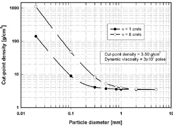
It can be found from eq. (1.26) that for particles greater than 1mm the hydrodynamic drag can be neglected and the cut point density is independent of particle size, and is given by eq. (1.23). However, by inclusion of the hydrodynamic drag, the cut point density begins to deviate, for particles smaller than 1 mm, from its “large particle value”, as illustrated in Fig.1.12.

Fig. 1.13 shows the inaccuracy in the cut-point density introduced by ignoring the hydrodynamic drag.

Figure 1.12 - The effect of hydrodynamic drag on cut-point density, for two particle velocities.

The nominal “large particle” cut-point density ρcp = 3500 kg/m

3 .

Figure 1.13 - The inaccuracy in cut-point density introduced by ignoring

hydrodynamic drag, for two different particle velocities. The nominal cut-point

1.6.4 Interaction of particles during separation

The analysis of the particle motion in a ferrofluid assumed that particles were non-interacting. This simplification ignores, however, the fact that non-magnetic particles suspended in a magnetic fluid possess surface magnetic charges as a result of magnetization of the surrounding fluid. It was determined, theoretically and experimentally, that non-magnetic particles, placed in a magnetized ferrofluid, attracted one another in the direction parallel to the direction of magnetic field and repelled one another in the perpendicular direction.

The situation is depicted in Fig. 1.8. The attractive force increases with increasing density of the ferrofluid and the magnetic field strength. The attractive interaction was found to reduce the selectivity of separation of non-magnetic particles in a magnetic fluid.

1.7 The Magnetic Density Separation

(MDS)

Many designs of magneto-hydrostatic separators are known from the literature. The most popular type of separator consists of a cavity between two curved polar pieces of an electromagnet, in which the field lines run mainly horizontal and the concentration of field lines (the magnetic induction) increases towards the bottom of the cavity. The curved poles create a field that produces an almost constant effective density of the magnetic fluid. An important problem of these separators is that magnetic contaminants are attracted to the poles. Another important point is the relatively complex geometry of the cavity and the difficulties of up scaling.

The approach to magneto-hydrostatic separation is to create a medium with a cut-density that is not a constant but varies with the vertical coordinate.

For a magnetic induction that varies exponentially with z,

2 / 0

( , , ) e z w

B x y z =B −π (1.28)

The effective medium density varies with z as well:

w z f a e gw MB π π ρ ρ 2 0 −2 + = (1.29)

A field like that of Eq. (1.28) can be created by a series of alternating magnetic poles in a plane geometry: 2 / 0 2 / 0 ( , , ) e sin(2 / ) ( , , ) e cos(2 / ) z w x z w z B x y z B x w B x y z B x w π π π π − − = = (1.30)

The magnetic density separator segregates the feed into layers of different materials, with each material floating on a distance from the magnet according to its density and the apparent density of the fluid.

If two materials of density ρ1 and ρ2 need to be separated, the segregation distance:

2 1 2 1 ln 2 w z z

ρ

ρ

π

ρ

ρ

must exceed the maximum particle size of the feed. This is achieved by selecting a proper wavelength w of the field for the application.

1.8 The magnet

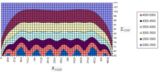
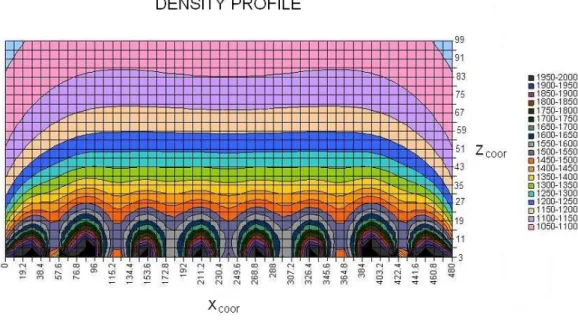
Professor Rem of the Delft University of Technology calculated a configuration of magnets that would produce such a field. Magnet manufacturers Bakker Magnetics, who specializes in the manufacture of complex magnet systems, produced the configuration. The main ingredient of the magnet plate is a set of extremely powerful permanent iron neodymium-borium magnets. The field strength just above the magnets is 1 Tesla, which is strong for a permanent magnet. The magnets are mounted in a ‘frustrated’ configuration, which means that they are out of balance and subject to large forces acting between them. The whole assembly is covered by a steel plate to protect researchers from being hit by any magnet fragments that may become detached from the main mass. The magnet configuration calculated by Professor Rem is a patent, and is thus secret. The apparent density of the fluid depends solely on the vertical distance from the magnet’s surface. All density lines run horizontal, creating an apparent density range which is the same everywhere on the magnet. The magnet used in this project created however a density profile in which a wavy pattern starts to appear when approaching the magnet’s surface: a few centimeters above the magnet the density lines are horizontal, but closer to the surface waves are appearing whose amplitudes are increasing towards the magnet’s surface. Since particles will settle in the trough of a wave, the floating height of particles decreases when this height lies in the wavy part of the density profile. The closer the floating height is to the magnet’s surface, the larger this decrease will be. In the first few centimeters above the magnet the wavy pattern has even such large amplitudes that low density trenches are created: relative light particles will sink when entering the fluid. Is thus important that the particles that are to be extracted hover at a vertical height where the effect of the trenches cannot be seen anymore.

Chapter 2

2.1 Magnetic density separator: original layout

A separator, which is able to separate multiple density fractions at once, was designed. The main part of the separator is a brass vibrating gutter. Fluid and non-ferrous materials are led into the gutter, straight into the magnetic field where the separation begins. At the end of the magnetic field the different density fractions are pumped towards a sieve. Here the materials remain behind and the fluid is collected and circulated.

Figure 2.2 - Process of Magnetic Density Separation (MDS): layout and equipment. Figure 2.1 - Process of Magnetic Density Separation (MDS): original layout.

The separation process consists of five steps:

1. Fluid that is collected at the end of the separation process is circulated back to the beginning, where it is led through a laminator in order to create a laminar flow. The laminator is a 100 mm long grid with rectangular openings that leads the fluid into the magnetic field.

2. The minerals are fed into a section of the gutter, where they are mixed with a small amount of magnetic fluid. A stirrer is used to make sure the samples are drawn downwards to the particle inlet. The section is connected to the main separation area by a hose which leads the minerals through the laminator in a special inlet.

3. Once in the separation area, the minerals move towards their floating heights. During the separation the gutter vibrates at high frequency with low amplitude. This way the minerals do not get stuck to the bottom or side walls of the gutter.

4. At the end of magnetic field the materials are separated permanently by outlets, each one 10 mm high. The fluid and the minerals are led towards a

s

Figure 2.5 - Sieve divided into 10 sections. Figure 2.4 - Outlets sections.

small opening. Each opening has a separate pump, which pumps the fluid and the particles towards a sieve. The sieve is divided in ten sections, each connected to one outlet.

5. The different fractions are collected in the sieve and the fluid is retrieved in an area, which is connected to the beginning of the separator. The fluid is led back to the separator through a series of pipes. The fluid flow is controlled by two valves.

2.2 First test: separating diamonds from gangue

minerals

In its first application the magnetic density separator was used to separate the diamond fraction - represented from 0,5 ÷ 2 mm olivine particles - from other equally small gangue materials. The aim of this test was to extract a single density fraction from the fluid, while all material lighter or heavier is discarded.

2.2.1 Materials

A diamond crystal has a mean density of 3520±10 kg/m3. Due to inclusion of gases and minerals this density can range from 3100 ÷ 3600 kg/m3. To extract all diamonds, material outside the density range of 3100 ÷ 3600 kg/m3 should be discarded. To ensure a high grade of pureness of the diamond fraction it is important that not too many other minerals report to this fraction. Since hydrostatic magnetic separation can already discard up to 95% of the particles using densities of 2700 ÷ 3100 kg/m3 and with magnetic density separation being capable of rejecting the heavy minerals (>3600 kg/m3) as well, using magnetic density separation will only improve the separation results.

The materials used for this test were orthoclase (2515 kg/m3), calcite (2697 kg/m3) olivine (3359 kg/m3) and ilmenite (4710 kg/m3). Due to its density the olivine was suitable to represent the diamond fraction during the tests. The materials were chosen on the basis of the colour. The distinct colour differences between the minerals can be used to get a first impression on the separation result; X-Ray Fluorescence (XRF) was used to determine the recovery of each mineral in the separation fractions.

2.2.2 The fluid

The fluid used originates from Ferrotec. A magnetization M=13500 A/m and a density ρf =1360 kg/m3 were measured for the pure fluid. To create a suitable

density range for separation the magnetic fluid was diluted using water.

It can be seen that low density trenches are present in the first 25 mm above the surface of the magnet. It was therefore decided that the olivine should have a floating height of at least 30 mm so the mineral’s particles would not be hindered by the trenches. It was decided to use a fluid with dilution factor 1:3, consisting of one part of magnetic fluid mixed with two parts of water. Theoretically the floating height of olivine in a 1:3 fluid is 40 mm. From experimental floating-test was determined that, even though the wavy pattern in the density profile decreases the floating height of olivine, it still remains over 30 mm.

2.2.3 Time of separation

Based on the theoretical floating height in the 1:3 fluid it was calculated how much time a mineral particle needs to reach its floating height. The 0,5 mm orthoclase particles take the longest time to separate: 0,62 seconds. Since the separation area in the separator is 0,30 m long, the fluid velocity in the separator should be less than 0,30 / 0,62 = 0,48 m/s for all minerals to successfully reach their floating heights.

Figure 2.6 - Density profile in a ferrofluid with a dilution factor of 1:3 and a

magnetization of 4500 A/m.

It should be noted that the olivine particles are inserted at their experimental floating height, so in practice they already float at their extraction height.

2.2.4 Flow measurements

For magnetic density separation a laminar flow was preferred. If the flow is turbulent, the mineral particles could end up in the wrong density fraction, disrupting the separation process.

To test the flow inside the separator the system was filled with water and a small amount of ink was injected in the main stream at different heights. The ink clouds moved horizontally from inlet toward outlet. This indicated that no misplacement of particles should take place inside the separator due to turbulence.

To measure the flow speed of the magnetic fluid inside the separator, an electromagnetic flow sensor (EM) was used. This sensor can measure in the low velocity range of 0 ÷ 1 m/s and it can measure the velocity at different heights, so a velocity profile through the fluid column in the separation area could be made. Since the EM sensor works with a self generated magnetic field, the measurements could only be done with the magnet removed from under the separator. The fluid velocity was measured at three different locations (about 6 cm behind the laminator, halfway the separation area and about 6 cm in front of the outlets), at four different heights. It was assumed that the velocities measured in magnetic fluid will be comparable to those in water, to which the sensor is calibrated. 0,02000 0,02500 0,03000 0,03500 0,04000 0,04500 0,05000 0 0,020,040,060,08 0,1 0,120,140,160,18 0,2 0,220,240,260,28 0,3 0,320,340,360,38 0,4 0,420,440,460,48 0,5 0,520,540,560,58 0,6 0,620,64 time (seconds) flo a tin g h e ig h ts f ro m t = 0 ( m ) orthoclase 0.5 mm orthoclase 2 mm calcite 0.5 mm calcite 2 mm olivine 0.5 mm olivine 2 mm ilmenite 0.5 mm ilmenite 2 mm

One trend is that the fluid velocity decreases with depth. Since the fluid column in the separator is only 10 cm high, the bottom will have a relative large influence on the fluid’s velocity. Another observation that can be made is that the amount of fluid transported halfway the laminator is almost the same as the amount of fluid transported near the outlets. To transport about the same amount of fluid velocities at lower heights should decrease.

The reliability of the measurements is low since the amount of fluid transported near the laminator is much lower than the amounts transported at the other two locations. Close to the laminator and near the particle inlet, which is placed at a height of 3 ÷ 4 cm from the magnet’s surface, the flow is more turbulent. The large difference with the other two locations can partly be caused by this turbulence. Not only is the EM sensor designed for measurements in laminar flow, its large probe size causes some disturbance in the flow as well. The probe used for the measurements was 3 cm wide, while the separation area was 6 cm wide.

2.2.5 Results

It was found that olivine, calcite and orthoclase ended up in lower separation fractions than predicted. The most olivine and ilmenite ended up in the first two fractions, 1 ÷ 3 cm above the magnet, while a larger part of the lighter calcite and orthoclase were found in fraction three and higher (3 ÷ 6 cm above the magnet). The total recovery of olivine in the first two fraction was 93,6%. This shows a high recovery rate for olivine (and thus diamond fraction).

average recovery test 1 and 2

0 0,1 0,2 0,3 0,4 0,5 0,6 0,7 0,8 0,9 1 1 2 3 4 5 fraction re c o v e ry ilmenite olivine calcite orthoclase

Figure 2.8 - Results about separation test of diamonds.

2.2.6 Problems found during experimentation

The apparent density of the fluid depends solely on the vertical distance from the surface of the magnet. All density lines run horizontal, creating an apparent density range which is the same everywhere on the magnet.

The magnet used in this project created however a density profile in which a wavy pattern starts to appear when approaching the magnet’s surface: a few centimetres above the magnet the density lines are horizontal, but closer to the surface waves are appearing whose amplitudes are increasing towards the magnet’s surface. The floating height of particles decreases when this height lies in the wavy part of the density profile. The closer the floating height is to the magnet’s surface, the larger this decrease will be. In the first few centimetres above the magnet the wavy pattern has even such large amplitudes that low density trenches are created: relative light particles will sink when entering the fluid. Is thus important that the particles that are to be extracted hover at a vertical height where the effect of the trenches cannot be seen anymore.

Moreover it was noted that during the lab-scale tests all minerals ended up in lower separation fractions. The lower recovery heights can be explained by the density profile which slopes downwards near the magnet’s edges. When particle enter this part of the profile, their floating heights decrease.

The flow

The turbulence near the laminator can be minimized when the particle inlet velocity is matched with the fluid flow through the laminator. This can be done by using pumps to control the return flow instead of letting the fluid flow freely back to the separator through a series of pipes.

The acceleration of the fluid at high levels near the outlets (and thus deceleration of the fluid velocity near the magnet’s surface) can be better controlled by regulating the pump separately. All pumps at the outlets are set to the same capacity. Assuming a laminar flow is present in the separation area, the volume of fluid entering the lower pumps is less than the fluid entering the higher pumps. For all pumps to reach the same capacity, the lower pumps need extra fluid. If this fluid is withdrawn from higher fluid levels, this will slow down the fluid that is already flowing at pump level. To avoid this effect it is recommended to use