Alma Mater Studiorum – Università di Bologna
DOTTORATO DI RICERCA IN
Geofisica
Ciclo XXVI
Settore Concorsuale di afferenza: 04/A4 Settore Scientifico disciplinare: GEO/10
TITOLO TESI
Numerical modeling of the Alto Tiberina
low-angle normal
fault mechanics
Candidato Relatore
Luigi Vadacca Dr. Emanuele Casarotti Coordinatore Dottorato
Prof. Michele Dragoni
Abstract
The aim of this Thesis is to obtain a better understanding of the mechanical behavior of the active Alto Tiberina normal fault (ATF). Integrating geological, geodetic and seismological data, we perform 2D and 3D quasi-static and dynamic mechanical models to simulate the interseismic phase and rupture dynamic of the ATF. Effects of ATF locking depth, synthetic and antithetic fault activity, lithology and realistic fault geometries are taken in account. The 2D and 3D quasi-static model results suggest that the deformation pattern inferred by GPS data is consistent with a very compliant ATF zone (from 5 to 15 km) and Gubbio fault activity. The presence of the ATF compliant zone is a first order condition to redistribute the stress in the Umbria-Marche region; the stress bipartition between hanging wall (high values) and footwall (low values) inferred by the ATF zone activity could explain the microseismicity rates that are higher in the hanging wall respect to the footwall. The interseismic stress build-up is mainly located along the Gubbio fault zone and near ATF patches with higher dip (30°<dip<37°) that we hypothesize can fail seismically even if a typical Byerlee friction (0.6-0-75) is assumed. Finally, the results of 3D rupture dynamic models demonstrate that the magnitude expected, after that an event is simulated on the ATF, can decrease if we consider the fault plane roughness.
Contents
1. Introduction……….………..……..……….... 5
2. The Alto Tiberina low-angle normal fault……...…………..……….…………...7
2.1. Introduction………...7
2.2. Tectonic setting………..………...7
2.3. Seismicity………..……….…….9
2.4. Long-term and short-term deformation…………..………...……10
2.5. Geometries………...…...…..12
2.6. Frictional reactivation theory for normal faults………15
2.7. Open questions………...………...17
3. Numerical method………...………...18
3.1. Introduction………...………18
3.2. Finite element method (FEM)………...…………18
3.2.1. Comsol Multiphysics………...…………19
3.2.2. PyLith………...………...………20
3.3. Spectral element method (SEM)………...……21
3.3.1. SPECFEM3D………...……...22
3.4. Fault implementation………...….……….24
4. Modelling the interseismic deformation of the Alto Tiberina fault system by 2D numerical simulations: locking depth, fault activity and effects of lithology……….………26
4.1. Introduction………...……26
4.2. Modelling description……...………...……….27
4.3. Model results………...37
4.3.1. ATF locking depth effects……….………..37
4.3.2. Synthetic and antithetic fault activity effects….………...……40
4.4. Discussion and concluding remarks………53
5. Modelling the interseismic deformation of the Alto Tiberina fault system by 3D numerical simulations: fault roughness effects…………...57
5.1. Introduction………...57
5.2. Model description………..57
5.3. Model results……….61
5.4. Discussion and concluding remarks………..63
6. Rupture dynamics from 3D Alto Tiberina rough-fault numerical simulations.……….70
6.1. Introduction………...70
6.2. Rupture dynamic modeling setup ……….71
6.3. Results………...76
6.4. Discussion and concluding remarks……….……….80
7. Conclusions……….82
References 84
1. Introduction
1.1. Overview of the problem
The low-angle normal faults (LANFs) are a particular class of normal faults characterized by very low dips (0-30°). Initially discovered in the Basin and Range province, US, (Anderson, 1971; Longwell, 1945; Wernicke, 1981), then they have been recognized in most other extensional tectonic setting (e.g. Collettini, 2011). Geological evidences indicate that several LANFs originated and slipped in the brittle crust as primary, gently dipping normal faults (Wernicke et al., 1985; Wernicke, 1995; Axen, 2004). Moreover large displacements are associated at these faults, which are active within a crustal stress field characterized by vertical σ1 trajectories (Collettini and Holdsworth, 2004; Hayman et al., 2003; John and Foster, 1993; Jolivet et al., 2010; Lister and Davis, 1989). Active LANFs are proposed in Papua New Guinea, Gulf of Corinth (Greece) and Apennines on the base of seismological data (Chiaraluce et al., 2007; Abers et al., 1997; Rietbrock et al., 1996) even if there are no strong evidences for large (M > 6) earthquakes triggered along these structures (Jackson and White, 1989; Collettini and Sibson, 2001).
Since when the LANFs have been discovered, the scientific community debate around two principal questions: a) how can they be born in the brittle crust and b) how can they accommodate the extension. In fact, these faults are not conform to the fault mechanical theory that predicts only steep (about 60°) normal faults in the brittle crust (Anderson, 1951) and frictional lock up of existing normal faults at 30° dip (Collettini and Sibson, 2001; Sibson, 1985) considering a typical 0.7 friction coefficient (Byerlee, 1978); then, for dip less then 30°, new steep faults should form.
We tackle the second issue (b) by considering the Altotiberina fault, an active low-angle normal fault cutting the brittle crust of Northern Apennines with an average dip of 17°. In this work, integrating geological, seismological and geodetic data we use the finite element method to model the interseismic phase of the Alto Tiberina Fault system. At first, through 2D numerical simulations we investigate the effects of ATF locking depth, synthetic and antithetic fault activity and lithology on the deformation rates and stress build-up (Chapter 4). Then we evaluate these effects performing 3D numerical models that include a realistic geometry of the Alto Tiberina fault plane (available on the basis on seismic reflection profiles; Mirabella et al., 2011) and characterized by strong dip-angle variations (Chapter 5). Finally we discuss the rupture dynamic problem on rough faults. For this purpose, through spectral element method numerical code, we investigate the geometrical effects of a simulated earthquake on the Alto Tiberina fault in terms of maximum magnitude (Chapter 6).
2. The Alto Tiberina low-angle normal fault
2.1. Introduction
The Alto Tiberina fault (ATF) is a 70 km long low-angle (about 17°) normal fault East-dipping in the Umbria-Marche Apennines (Central Italy) and characterized by SW-NE oriented extension and rates of 2-3 mm/yr. Striated geological fault planes (Lavecchia et al., 1994), focal mechanisms and borehole breakouts (Montone et al., 2004) define a regional active stress field with a nearly vertical σ1 and NE trending subhorizontal σ3. In this area historical and instrumental earthquakes mainly occur on
West-dipping high-angle normal faults. Within this tectonic context, the ATF has accumulated 2 km of displacement over the past 2 Ma, but the deformation processes active along this misoriented fault, as well as its mechanical behavior, are still unknown. In this chapter we present a review of the main geological and seismological aspects that outline the ATF mechanical behavior.
2.2. Tectonic setting
The northern Apennines consists of a NE verging thrust-fold belt formed as the result of the collision between the European continental margin (Sardinia-Corsica block) and the Adriatic lithosphere (e.g., Alvarez, 1972; Reutter et al., 1980). From the Oligocene to the present-day, the area has experienced two phases of eastward migrating deformation: an early compression with eastward directed thrusting and a later phase of extension (e.g., Elter et al., 1975; Pauselli et al., 2006). The interpretation of the seismic reflection profiles (Pialli et al., 1998) shows that a
significant amount of extension within the brittle upper crust is accommodated by a system of East dipping LANFs with associated high-angle antithetic structures (i.e. Chiaraluce et al., 2007). Older parts of the extensional system are significantly exhumed to the west in the Tyrrhenian islands (e.g., Elba) and Tuscany (Carmignani and Kligfield, 1990; Keller et al., 1994; Jolivet et al., 1998; Collettini and Holdsworth, 2004) while the ATF (Barchi et al., 1998; Boncio et al., 2000; Collettini and Barchi, 2002), which is the easternmost of these structures, is located in the inner sector of the Umbria-Marche Apennines (Figure 1) where an extensional stress field is active today.
Fig. 1. a) Seismicity in the northern Apennines. In white stars, historical earthquakes are shown. Red
symbols show the epicenters of the earthquakes recorded during the 2000–2001 seismic survey (Chiaraluce et al., 2007). Orange, blue and green symbols indicate the aftershocks of the 1984 Gubbio (Mw 5.1), the 1998 Gualdo Tadino (Mw 5.1) earthquakes and 1997 Colfiorito sequence respectively.
2.3. Seismicity
At present, the active extension region is concentrated in the inner zone of the Umbria-Marche Apennines where the strongest historical and instrumental (5.0 < M < 6.0) earthquakes are located (Figure 1). The seismicity does not follow the arc shape structures inherited from the previous compressional tectonic phase but clusters along a ∼30 km wide longitudinal zone (Chiaraluce et al., 2004; Chiarabba et al., 2005) where the historical earthquakes are also located (Figure 5a; Chiaraluce et al., 2007). In the past 20 years, three main seismic sequences have occurred in the ATF region: the 1984 Gubbio sequence (Mw 5.1), the 1997 Colfiorito sequence (Mw 6.0, 5.7 and 5.6), and the 1998 Gualdo Tadino (Mw 5.1) sequence (Figure 5). All the mainshocks are related to SW dipping (∼40°) normal faults, with fault plane ruptures dipping in
the opposite direction to the ATF. In this region there is an important contribute of fluid overpressure on the seismicity as interpreted for the Colfiorito sequence (Miller et al., 2004; Antonioli et al., 2005). During a temporary seismic experiment, Chiaraluce at al. (2007) recorded ∼2000 earthquakes with ML 3.1. The
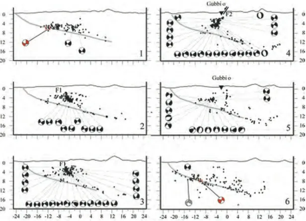
microseismicity defines a 500 to 1000 m thick fault zone that crosscuts the upper crust from 4 km down to 16 km depth. The fault coincides with the geometry and location of the ATF as derived from geological observations and interpretation of depth-converted seismic reflection profiles (Figure 2). In the ATF zone, Chiaraluce et al. (2007) also observe the presence of clusters of earthquakes occurring with relatively short time delays and rupturing the same fault patch. To explain movements on the ATF, oriented at high angles (∼75°) to the maximum vertical principal stress,
strengthening areas while microearthquakes occur in velocity weakening patches by fluid overpressures.
Fig. 2. Microseismicity location compared with the ATF plane for different cross-sections from NW to
SE (courtesy of Chiaraluce et al., 2007).
2.4. Long-term and short-term deformation
On the basis of the long‐term extensional values obtained through cross-‐section
balancing, Mirabella et al. (2011) inferred a 3 mm/yr long-‐term extension rate in the study area. Very similar values (2.7– 3.0 mm/yr) have been calculated through GPS measurements for the present-‐day extensional rate in northwestern Umbria (Figure 3;
ATF system and has been a nearly steady state process through time (Mirabella et al., 2001).
Fig. 3 Crustal deformation in Umbria-March region, Italy. We can observe a velocity gradient from
SW to NW with a maximum extension of 2.5-3 mm/yr in the central part of the study area. In magenta the ATF isobaths. Note that the extension is concentrated across a ∼30– 40 km wide zone (green dotted line; Serpelloni, p.c.).
The present-day extensional strain in the northern Apennines inferred from geodetic data is concentrated across a ∼30– 40 km wide zone (Figure 3) that coincides with the area struck by the strongest earthquakes (Figure 4). Hreinsdottir and Bennett (2009) obtained the same extensional rate remarking that the ATF in the Northern Apennines is actively slipping at a shallow depth within the brittle crust.
2.5. Geometries
The knowledge of the fault plane geometry is a priority for interseismic and rupture dynamic modeling studies. Moreover, a good crustal velocity model is necessary to understand where local stress accumulations occur. Miller et al. (2004) through geophysical data have identified the Triassic Evaporites as the source region of the major extensional earthquakes of the Northern Apennines (M ∼6). For this reason, in
this paragraph we analyse the structural setting where the ATF is located.
Figure 4a shows the geological map of the study area. We consider the S3 cross section (Figure 4b) for this structural analysis. From the surface to the depth four principal seismostratigraphic units are recognized (Mirabella et al., 2011): Turbidites (Vp= 4.00 Km/s); Carbonatic multilayer (Vp = 5.50 km/s); Evaporites (Vp= 6.10 km/s) and Phyllites (or Basament s.l.; Vp= 5.00 Km/s). These units have been dislocated by the activity of several synthetic and antithetic normal faults that intersect the ATF with depth. The most Eastern antithetic fault (Gubbio fault) is constituted by a typical geometry flat-ramp. This feature is associated at a pre-extensional stage of the Gubbio fault activity related to the evolution of the Miocene foredeep (Mirabella et al., 2004). Instead, the ATF is associated entirely at the last extensional phase (Mirabella et al., 2011). It is possible recognize, simply by the S3 cross-section, a staircase geometry for the ATF
a)
b)
Fig. 4. a) Geological map of the study area. b) Geological-structural cross-section cutting the inner
The three-dimensional ATF fault geometry is well known by the interpretation of seismic profiles (Figure 5; Mirabella et al., 2011). Figure 6 shows the reconstruction of the ATF fault plane starting from the isobaths of Mirabella et al. 2011. Along-dip and along-strike irregularities and strong variation of the immersion slope are evident. The fault dip ranges from minimum value near to a flat plane to maximum values of 37° (Figure 6). This feature is very important in terms of well-orientation plane
following the theory of reactivation, as discussed in the next paragraph.
Fig. 5. Isobath map of the ATF reflector. The thick lines are the depth contours drawn every kilo-
meter, the thin lines are the depth contours every 250 m, the dotted lines are the sampled seismic lines from which the contours have been drawn (Mirabella et al., 2011).
Fig. 6. ATF geometry obtained by the isobath map of Mirabella et al. (2011). We plot the dip
distribution of the fault plane.
2.6. Frictional reactivation theory for normal faults
Following the analysis of Sibson (1985) and Collettini (2011) the re-shear of existing cohesionless faults with coefficient of sliding friction, μ, can be defined by Amontons'
law:
τ = μ (σn – Pf) (1)
Then, for the two-dimensional case in which an existing fault containing the σ2 axis lies at a reactivation angle θr to σ1, Eq. (1) may be rewritten in terms of the effective
principal stresses (Sibson, 1985; Collettini, 2011) as:
which reduces to
R = (σ’1/σ’3) = (1 + μ cot θr)/ (1 - μ cot θr) (3)
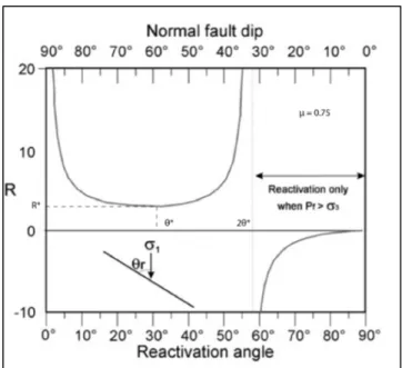
Eq. (3) defines how easy is to reactivate a fault as a function of θr (Sibson, 1985). The stress ratio for reactivation R is plotted against θr for the particular case of μ = 0.75 in
Figure. 7. R has a minimum positive value R* = ( 1 + 𝜇2 + µ)2 at the optimum angle for frictional reactivation given by θ* = ½ tan-1 (1/μ), but increases to infinity for θ
r = 0 and θr = 2θ*. For μ = 0.75, θ* = 26.5° with R* = 4. For θr> 2θ*, R< 0 which requires σ’3< 0, therefore the effective least principal stress must be tensile (Sibson, 1985).
Fig. 7. Stress ratio, R, for frictional reactivation of a cohesionless fault plotted against the reactivation
In this way, the re-shear is only possible for overpressure conditions where Pf > σ3. However, the tensile overpressure condition is difficult to be maintained because hydrofractures formed when Pf = σ3 + T (where T is the tensile rock strength) draining off the pressurises fluids (Collettini, 2011). For this reason particular friction condition are necessary to reactive a misoriented fault (e.g. μ< 0.6).
2.7. Open questions
The principal features of the ATF can be so summarized: 1) it is an active low angle normal fault dipping ∼20° in the brittle crust; 2) the fault is constituted by a finite plane larger than 2.7・103 Km2 suggesting that a maximum M ∼7 earthquake could
occur in case of rupture propagating along the entire fault-‐surface (Mirabella et al.,
2011); 3) the fault roughness is characterized by strong along-dip and along-strike irregularities. All these features are not yet sufficient to delineate a precise mechanical behavior for this fault and many questions have yet to find answers. Hence first question is: what is the effect of ATF system (ATF + other faults) on the interseismic deformation? And where the maximum interseismic stress build-up is expected? Another important aspect concerning the roughness associated at the ATF since the geometrical irregularity of the fault plane can generate a strong redistribution of the interseismic stress. Even the dynamic of the rupture can be influenced by that accentuated roughness.
3. Numerical method
3.1. Introduction
In this Chapter, two different numerical methods to resolve the partial derivate equations (PDE) are discussed: the finite element method (FEM) and the spectral element method (SEM). The FEM will be use to resolve quasi-static problem in order to simulate the interseismic phase in Chapter 4 and 5. The SEM will be adopted to simulate dynamic ruptures of the ATF in Chapter 6. We examine the principal features of these methods and a short description of the numerical codes adopted in this thesis.
3.2. Finite element method (FEM)
The FEM is a computational technique that describes the deformation state of a continuum system through the solution of PDEs at one or more variables, with a note analytic shape and defined in small regions of the continuum (Islail-Zadeh and Tackley, 2010). The method needs to discretize the system, that is to divide it in a equivalent system of a small structures (elementary components). In this way the solutions are formulated for every unit and combined to obtain the solution of the original structure. The smaller the elementary components are, the closer the system is to the continuum case, the greater the complexity of the solution becomes. Generally, it needs to research a good compromise between accuracy, numerical cost and complexity of the studied problem.
The system so defined has configured in the way that displacement and stress are continue from one element to the other, that internal stress is in equilibrium and that the boundary conditions are satisfied. In a FE analysis, we have to consider three types of fundamental relations: a) the geometrical relationship between strain and displacement, called equations of compatibility; b) the constitutive relation of the material; c) the equilibrium equation.
The approximation process requests to discretize the continuum system through different steps: the continuum media is divided in elements; the elements are connected through nodes located on the vertices (the displacements of the nodes define the incognita of the problem); we choose an interpolation criterion that defines the displacement in every point of the element as function of the displacement at the nodes; the strain is calculated from the displacement and from the strain, through the constitutive relations of the material, can be obtained the stress; the system of forces so constituted have equilibrated the internal stress and the external load applied. Every approximation during the process introduces an arbitrary degree in the solution, for this the described step should be performed with maximum cure.
3.2.1. Comsol Multiphysics
Comsol Multiphysics is the software that we adopted for 2D quasi-static models of ATF. It is a commercial FEM software that consents to resolve many scientific problems with a multiphysics approach, through the coupling of different physics described by a system of PDEs. The code provides the possibility to define geometries, physics parameters, material properties, loads and boundary conditions.
In Comsol, it is also possible to define equations ad hoc used by the code in combination of the PDEs to resolve specific problems. The package can be used by a graphic interface that permits to operate in all modelling phases in simple way, starting to build the geometry directly in the code o importing it from other CAD software. The geometry is discretized by triangular or quadrilateral elements.
3.2.2. PyLith
PyLith (Aagaard et al., 2013) is the numerical code adopted for 3D quasi-static simulation of ATF interseismic phase. PyLith is open source, ad-hoc designed for 3-D dynamic and quasistatic simulations of crustal deformation, primarily earthquake and volcanoes. PyLith is one component in the process of investigating tectonic problems (Figure 8). Given a geological problem of interest, it need first provide a geometrical representation of the desired structure. Once the structure has been defined, a computational mesh must be created. PyLith provides three mesh importing options: CUBIT Exodus format, LaGriT GMV and Pset files, and PyLith mesh ASCII format. Present output consists of VTK or HDF5/Xdmf files which can be used by a number of visualization codes (e.g., ParaView, Visit, MayaVi, and Matlab).
Fig. 8. Workflow involved in going from geologic structure to problem analysis (courtesy of Aagaard
et al., 2013).
3.3. Spectral element method (SEM)
Spectral element method (SEM) is a high-order accurate and flexible method originally introduced in computational fluid dynamics (Patera, 1984) and after has been successfully applied in seismic wave propagation (Komatitsch et al, 2005; Chaljub et al, 2007). Recently this method is finding new perspectives in the earthquake dynamic too (Kaneko et al., 2008; Ampuero, 2009; Galvez et al., 2013). The main features of this method can be so summarized: 1) In contrast to many numerical methods, such as finite-difference and pseudospectral methods that are based upon a strong formulation of the problem (they work directly with the equation of motion) SEM (like FEM) is based upon the weak formulation of wave or integral
equation. 2) Simulation volumes are discretized using a grid (mesh) of hexahedral elements. This mesh can honour any discontinuity in the model and can be fully unstructured (i.e., the number of elements that share a given point can vary and take any value), thus very complex geometries and any arbitrary shaped domain can be accommodated. Using hexahedral elements leads to several benefits, such as optimized tensor products, a diagonal mass matrix and a smaller number of elements compared to tetrahedral meshing (Peter et al., 2011). Mechanical properties can vary inside each element, allowing fully heterogeneous media to be implemented. 3) SEM uses high-degree (between 4 and 10) Lagrange polynomials as basis functions. This ensures a very high spatial accuracy and an exponential decreasing of errors typical of spectral and pseudo-spectral methods. 4) Very efficient implementation on parallel computers with distributed memory. This tremendously reduces the computational costs, making SEM suitable to be used for large, high-resolution simulations on very powerful machines.
3.3.1. SPECFEM3D
In this work, to resolve the problem of the ATF dynamic rupture, we use SPECFEM3D, an open source code that uses the spectral element method and built ad hoc to resolve wave propagations and earthquake dynamic problems. The code finds application in highly complex 3D heterogeneous media. The workflow consists in different step-by-step operations as shown in figure 9. Starting from a detail geological and tomographic model the first crucial step is the meshing. The mesh in SPECFEM3D can be built in three different ways. The first option is using meshfem3D, a tool included in the code. It allows to design relatively simple mesh for
layercake models, using an analytical linear interpolation from the top to the bottom of the mesh (Peter et al., 2011).
Fig. 9. Workflow for running spectral-element simulations with SPECFEM3D. The gray box on top
contains the input elements for the code (courtesy of Magnoni, 2012).
For complex geometries, in particular in presence of strong discontinuity like faults, is possible to use CUBIT (Blacker et al., 1994) an external 3D unstructured mesh generator. The third possibility is using GEOCUBIT, a Python script collection based upon CUBIT (Casarotti et al., 2008). After that the mesh is built, it came partitioned in different slices through a software packages SCOTCH (Pellegrini and Roman, 1996). Every slice will be distributed for every core on the cluster (Fig. 10). After meshing and partitioning is possible to generate a database to assign the material and fault property. The last input to run the simulations are the definition of the location of receivers. At the end, the spectral-element solver performs a numerical integration of the wave equation, simulating the synthetic waveforms for each of the considered stations.
Fig. 10. Mesh partitioned using SCOTCH to run in parallel on four cores. The four partitions are
indicated by different colors (courtesy of Peter et al., 2011).
3.4. Fault implementation
In order two create relative motion across the fault surface in the finite-element mesh, two different methods are used in Comsol and PyLith codes (Fig.11a-b). In Comsol the fault is defined as a contact pairs. These pairs define boundaries where the parts may come into contact but cannot penetrate each other under deformation. The frictional constitute law is defined along this contact surface.
The boundaries where the fault is defined are splitted apriori before that the mesh is built. In this way the contact is constituted by different nodes with different index and are bound together by the cohesion forces (Fig. 11a). The boundaries of the contact pairs are called master and slave. For definition the slave cannot penetrate in the master boundary. In this way in order to facilitate the convergence is preferably that the slave identifies the hangingwall and the master boundary the footwall of the fault. This is because when, in the interseismic model, a gravity load is applied the slave is
the boundary from which the pressure comes and the master is the boundary that undergoes the pressure.
Differently, in PyLith additional degrees of freedom are added along with adjustment of the topology of the mesh. These additional degrees of freedom are associated with cohesive cells. These zero-volume cells allow control of the relative motion between vertices on the two sides of the fault. PyLith automatically adds cohesive cells for each fault surface. Figure 11b illustrates the results of inserting a cohesive cell in a mesh consisting of two quadrilateral cells. The great advantage of PyLith respect to Comsol is that different friction constitutive law are already implemented in the code. In SPECFEM3D, as in Comsol, the fault is implemented splitting the surface, directly in the mesher (Day et al., 2005, Galvez et al., 2013)
Fig. 11. Example of fault implementation for quadrilater cells. a) In Comsol the nodes are splitted
apriori; (b) in PyLith a cohesive cell is inserted into a mesh. The zero thickness cohesive cell (shown with dashed lines) controls slip on the fault via the relative motion between vertices 3 and 7 and 2 and 6 (like in the Comsol code, after Aagaard et al., 2013).
4. Modelling the interseismic deformation of the Alto Tiberina fault system by 2D numerical simulations: locking depth, fault activity and effects of lithology
4.1. Introduction
A critical issue of active low-angle normal faults (LANFs) is the identification of their mechanical behaviour. In fact, being misoriented faults with principal stress axis σ1, the large displacement and the lack of large earthquakes associated at these structures could be explained with a stable sliding behavior (Collettini, 2011).We take this issues considering the study case of the Alto Tiberina fault a very low-angle normal fault dipping ≈17° in the Northern Apennines (Figure 1). There are different ways to understand the mechanics behaviour of an active fault. These can be divided in inverse and direct methods. For example, geodetic inversions (e.g. Tong et al., 2013; Rolandone et al., 2008) and repeating earthquake localization (e.g. Turner et al., 2013) have been successfully used to define the creeping portion of the San Andreas Fault (another well known misoriented fault but in strike-slip regime). Friction laboratory experiments (direct methods) on rock samples of San Andreas Fault zone have confirmed those hypotheses (e.g. Carpenter et al., 2011).
Concerning the Alto Tiberina fault, Chiaraluce et al., (2007), during a temporary seismic experiment, have observed the presence of clusters of earthquakes occurring with relatively short time delays and rupturing the same Alto Tiberina Fault patches. They hypothesized a velocity strengthening rheology for the ATF zone with same fault patches with velocity weakening behaviour; moreover friction laboratory experiments on fault zone rocks of the Zuccale low angle normal fault, the natural
analogue of the ATF, showed a prevalent velocity strengthening rheology of the fault (Smith and Faulkner, 2010; Collettini et al; 2009).
In this Chapter, we show the results of 2D numerical mechanical models of the interseismic phase of the ATF system, constrained by geological, seismological and geodetic information. In particular we are going to analyse the following aspects: a) the ATF locking depth, b) the influence of the synthetic and antithetic faults activity and c) the influence of the lithology on the stress distribution and on the interseismic deformation rates.
4.2. Modelling description
We performed 2D finite element mechanical simulations with plain strain approximation by means of the commercial software COMSOL Multiphysics (http://
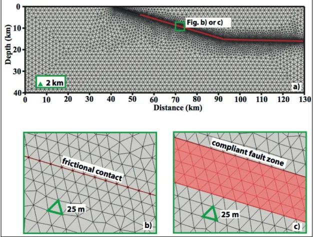
www.comsol.com/). We used a NE-SW regional cross-section cutting the central part of the ATF as base of the models (Figure 12 and 4) and considered only the faults associated at the ATF system defined by Mirabella et al. (2011). The mesh consists of approximately 270.000 triangular elements with a finest resolution of 25 m near the faults and decreases to 2000 m along the boundaries (Figure 19).
Fig. 12. Velocity map of the study area. The blue line represent the cross-section used for the 2D
models. In order to compare the velocity field obtained from the models with the data, we consider only the GPS stations whose distance from the cross-section is less then 10 km (the limit is represented by the dotted line); in particular the GPS stations considered are from SW to NE: SIO1, REPI, CSSB, VALC, UMBE, ATLO, MVAL, PIET, ATFO, ATBU, FOSS (thanks to Serpelloni for velocity vectors).
The crust is characterised entirely by an elastic rheology and we don’t consider differentiation between upper crust and lower crust rheology. This choice is justified since in this part of the Northern Apennines the brittle-ductile transition zone is very deep (25-30 km; Figure 1 and Pauselli and Federico, 2002). However, we extended the models until 40 km in order to avoid boundary effects.
In order to facilitate the convergence of the solution, the simulations were performed in two subsequent stages (Figure 13). In the initial stage, the model was subject only
In this way, the model compacts under the weight of the rocks and is brought in a stable equilibrium with gravity. In this first step, the boundary conditions, applied to all models, are the following: (a) the upper part of the models is free to move in all directions, (b) the SW and NE lateral boundaries of the crust and the bottom of the model are kept fixed in the direction perpendicular to these boundaries (slip parallel to these boundaries is allowed, Figure 13a). In the second stage (interseismic phase) we stretched the crust for 1000 years, applying a constant horizontal velocity of 0.5 mm/yr and 3.5 mm/yr on the SW and NE lateral boundaries respectively (Figure 13b) in according to the present-day plate kinematics of the Northern Apennines region (Hreinsdottir and Bennett, 2009; Serpelloni, p.c.). All the remaining boundary conditions are maintained.
The stress field resulting from the first stage is defined as uniaxial strain reference frame (Engelder, 1993). This state of stress is characterized by vertical stress Sv = ρgy (where ρ is the density, g is the gravity acceleration and y is the depth) and horizontal stress Sh = SH = (ν/(1 – ν)) * Sv, where ν is the Poisson’s ratio. In this way for ν = 0.25, the vertical stress is three times larger then the horizontal stress. If the obtained orientations of the stress axis are compatibles with those of the study area (Chiaraluce et al., 2007; Montone et al., 2004), the magnitude can be certainly away from reality. Because no constrain by stress measurements (e.g. leak off tests; Engelder, 1993) is available, a stress reference state is necessary. For this reason, the stress obtained during the second stage (extension phase) is not significative in absolute terms. Consequently, during the discussions of the results, we will consider only the tectonic stress, equal to the difference between the stress at end of the simulation and the stress obtained after the application of gravity.
Fig. 13. Boundary conditions for a generic model. a) During the stage1 a gravity load is applied. b)
During the stage 2, the crust is stretched applying a constant horizontal velocity of 0.5 mm/yr and 3.5 mm/yr on the SW and NE lateral boundaries. Note that these boundary conditions are the same for all models considered in this work.
In all models the faults are defined as 100 m thick shear zone. The weakness of the synthetic and antithetic shear zones is defined considering a Young modulus value of 100 MPa (two order of magnitude lower then the intact rocks; Tab. 2; Pasuselli and Federico, 2003), consistently with the typical Young’s moduli of unconsolidated rocks, as well as in situ measurements from various fault cores worldwide (Hoek, 2000; Schon, 2004; Gudmundsson, 2011). In this way when we will consider that these faults are active, it will means that they will have a Young modulus of 100 MPa (Tab. 2). Otherwise when inactive, the faults will have a Young modulus equal to that
evidences. In fact during the evolution of an active seismogenic fault, the Young modulus in the damage zone decreases due to the formation of new fractures. The same effect is obtained by the formation of gouge during earthquake rupture (e.g. Reches and Dewers, 2005). These factors reduce the effective Young modulus of the fault zone. By contrast, for an inactive fault, the effective Young modulus of the core and damage zone may increase because of healing and sealing of the associated fault rocks and fractures (e.g. Gudmundsson, 2004).
Otherwise, in order to simulate a free-slip motion along the ATF we consider a very compliant ATF zone with Young modulus value of 10 MPa. We have probed that a so -defined compliant fault zone has the same effects on the deformation rates respect to free-slip motion simulated along a contact with friction near to zero (Figure 14 and 15). The boundary conditions for this test are the same of figure 13 and the mechanical properties are listed in Table 1. Moreover we have assumed that the compliant fault zone and the free-slip contact are active below 5 km of depth (Figure 14). This method to simulate the ATF free-slip motion has the great advantage to reduce the computational costs and convergence problems respect to fault frictional contacts method. For this reason in all models we approximate the free-slip behaviour of the ATF as a compliant fault zone. We remark that in the following models the ATF is always active as a free-slip fault below the prescribed locking depth; above that the ATF is inactive (i.e. the Young modulus of the fault zone is equal to that of the intact rock, Tab. 2).
Fig. 14. a) Mesh used to test the frictional contact model (FC) b) and compliant fault zone model
(CFZ) c). The results are shown in figure 15. Note that the dimensions of the triangular mesh are maintained the same for both the models.
Intact rock ATF fault zone ATF fault
Young modulus (Pa) Poisson’s ratio Density (Kg/m3) Young modulus (Pa) Poisson’s ratio Density (Kg/m3) Friction coefficient Cohesion (Pa) FC model 5.33e10 0.25 2570 - - - ≈ 0 0 CFZ model 5.33e10 0.25 2570 1e7 0.35 2500 - -
Tab. 1. Mechanical properties used for FC and CFZ models (Figure 14-15) to test the effects of the
free-slip behaviour simulated via a fault frictional contact and a compliant fault zone. A Coulomb failure criterion is used for FC model.
Fig. 15. a) Horizontal velocity for the CFZ and FC models characterized by a different approximation
of the free-slip behaviour. The boundary conditions are the same of figure 13. Note that the horizontal component of the velocity is very similar for both the models.
Three different model settings are considered. First, we focus on the ATF locking depth and we consider four characteristic depths whence the ATF was in free-slip (2 km, 5 km, 8 km, 11 km; ATF models; Figure 16). The effects of the other faults are neglected. Moreover, to understand the only effects of the ATF locking depth, uniform elastic parameters for the crust are adopted (Table 2).
In the second set of models, we consider the influence of the activity of synthetic and antithetic faults on the interseismic deformation. We assume different configurations for every ATF locking depth previously considered: ATF2, ATF5, ATF8 and ATF11 models (Figure 17). Initially we consider that all the synthetic and antithetic faults are active (e.g. ATF2-a; Figure 17). Successively we consider inactive these faults (one-by-one from west to east,.e.g. ATF2-b-d; Figure 17). In the last model, only the antithetic Gubbio fault is active (e.g. ATF2-e; Figure 17). This set-up allows us to understand what faults is mainly accommodated the deformation. In these models, uniform elastic parameters for the crust are adopted (Table 3).
Finally, we consider the effects of the lithology on the interseismic stress build-up and deformation rates (ATF5-e-litho model, Figure 18). We consider only the principal
layers, representing lithological units characterized by similar competence (Pauselli and Federico, 2003; Mirabella et al., 2011; Table 4). In this model we assume that the Gubbio fault is active together with the ATF (that is instead free-slip).
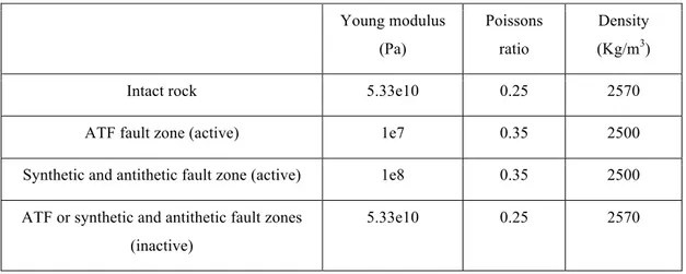
We maintain the same boundary conditions for the three different model settings as shown in figure 13. Young modulus (Pa) Poissons ratio Density (Kg/m3)
Intact rock 5.33e10 0.25 2570
ATF fault zone (active) 1e7 0.35 2500
ATF or synthetic and antithetic fault zones (inactive)
5.33e10 0.25 2570
Tab. 2. Mechanical properties used for ATF models (Figure 16) to test the effects of the ATF locking
depth.
Figure 16. ATF model set-up. In this configuration setting we explore the effects of the ATF locking
depth. We build four models for different ATF locking depth: ATFa (2km), ATFb (5 km), ATFc (8 km) and ATFd (11 km). Above the locking depth the ATF is inactive (see text). No effects of other faults are considered in these models. The crust is homogeneous (Tab. 2).
Young modulus (Pa) Poissons ratio Density (Kg/m3)
Intact rock 5.33e10 0.25 2570
ATF fault zone (active) 1e7 0.35 2500
Synthetic and antithetic fault zone (active) 1e8 0.35 2500
ATF or synthetic and antithetic fault zones (inactive)
5.33e10 0.25 2570
Tab. 3. Mechanical properties used for ATF2, ATF5, ATF8 and ATF11 models (Figure 17) to test the
effects of synthetic and antithetic fault activity for different ATF locking depth.
Figure 17. ATF2, ATF5, ATF8 and ATF11 model set-up. In this configuration setting we explore the
effects of the synthetic and antithetic fault activity for different ATF locking depth (2 km, 5 km, 8 km and 11 km). In this way for every ATF locking depth we build five different configurations depending on the synthetic and antithetic fault that are active. In ATF_a model all the faults are active. In ATF_b model configuration the faults 2, 3, 4 and 5 are active. In the ATF_c model the fauls 3,4 and 5 are active. Then in the ATF_d model only the antithetic faults 4 and 5 are active. Finally in ATF_e model only the Gubbio fault (5 or GF) is active. The symbol _ corresponds to 2, 5, 8 and 11 depending on the ATF locking depth considered. Above the locking depth the ATF is inactive. The crust is homogeneous (Tab. 3).
Young modulus (Pa) Poissons ratio Density (Kg/m3) Turbidites 3.17e10 0.25 2390 Carbonates 6.68e10 0.25 2660 Evaporites 8.65e10 0.25 2800 Pyllites 5.33e10 0.25 2570 Basament 9.21e10 0.25 2840
ATF fault zone (active) 1e7 0.35 2500
GF fault zone (active) 1e8 0.35 2500
ATF or synthetic and antithetic fault zones (inactive)
* * *
Tab. 4. Mechanical properties used for ATF5-e-litho model (Figure 18) to test the effects of the
lithology considering only the antithetic Gubbio fault active and for ATF locking depth of 5 km. (*) Note that in this model the inactive fault zones are defined with different elastic parameter values depending of the lithology that the fault intersects (e.g. if one inactive fault zone intersect the Turbidites, then it will have the same elastic parameters of the Turbidites; and so on).
Fig. 18. ATF-e-litho model set-up. In this model we explore the effects of the lithology. We consider
five main layers: Turbidites, Carbonates, Evaporites, Pyllites and Basament. The mechanical properties for every layers are shown in table 4. In this model we consider one ATF locking depth of 5 km and that only the Gubbio fault is active.
4.3. Model results
For each set of models we compare the horizontal velocity obtained by the different configurations with the GPS velocity measured during 10 years (Figure 12). We use 11 GPS stations whose distance from the cross-section is less then 10 km (from SW to Ne they are: SIO1, REPI, CSSB, VALC, UMBE, ATLO, MVAL, PIET, ATFO, ATBU, FOSS; Figure 12). Then, we evaluate the Von Mises stress, in order to quantify the interseismic stress build-up and have indication of shear stress.
4.3.1. ATF locking depth effects
Figure 19 shows the horizontal velocity field inferred from GPS data and numerical simulations for different ATF locking depth. The GPS data show an increase of the horizontal velocity from the High Tiber basin to the Gubbio basin (Figure 19). In this way the strain is localized in a 20 km wide area between two crustal blocks with rigid behavior (to SW and to NE, Figure 19). By comparing the results for the different locking depth we note that the best fitting was obtained for a 5 Km locking depth (see Table 5). Indeed, for a locking depth of 8 and 11 km, we observe that the horizontal velocities are underestimated respect to the GPS data. Nevertheless, for shallow locking depth (2 km), the horizontal velocities are overestimated.
Fig. 19. a) Horizzontal velocity for ATF model considering different ATF locking depth (2km, 5km, 8
km, 11 km). The mechanical property values for these models are shown in Table 2.The effects of other faults are neglected and an homogeneous crust is considered. Note the strain is mainly located in a 20 km wide area from the Tiber basin to the Gubbio basin (shown in b). The best fit is obtained for ATFb model (see Table 5).
Figure 20 shows the interseismic stress build-up after 1000 years and for different ATF locking depth. We can observe that high values of stress are localized near the tip point of the ATF generated by the free-slip along the fault. Moreover, for all different locking depth, we can recognize two prevalent areas at different stress magnitude: one localized in hanging-wall of the ATF with high values of stress, and another one situated in the footwall with lower values of stress.
Fig. 20. Interseismic stress build-up for ATF models considering different ATF locking depth (2 km, 5
km, 8 km and 11 km). The effects of other faults are neglected and an homogeneous crust is considered. Note that the only effect of the ATF locking depth generates a bipartition of stress concentration between hanging wall and footwall.
These models emphasize the main role of the ATF to accommodate the extension in this region. Nevertheless, the free-slip motion of this structure is not sufficient to explain the GPS data and the contribute of other faults could be so relevant.
4.3.2. Synthetic and antithetic fault activity effects
The effects of the synthetic and antithetic fault activity for different ATF locking depth on the horizontal velocity are here analyzed. In Figure 21, we show the results for a 2km ATF locking depth (ATF2 models). When all faults are considered active (ATF2a model), the velocity curve trend of the model is shifted towards higher values respect to the GPS data. The velocity trend of the models gradually improves when only the eastern faults are active (for example when only the antithetic faults are active; ATF2d-e models). The best fitting is reaching when only the Gubbio fault (GF) is maintained active.
The interseismic stress build-up for ATF2 model is shown in figure 22. We can observe that when all faults are considered active the stress accumulations in the ATF hanging-wall decrease (ATF2a model). In particular, more faults are active and more the stress build-up decreases. In fact when the Gubbio fault (GF, ATF2e model) is the only active structure the stress magnitude in the ATF hangingwall is reduced at values similar at the ATFe model (i.e when no synthetic and antithetic faults were active, Figure 20).
Fig. 21. Horizzontal velocity for ATF2 model. We explore different configurations of the synthetic and
antithetic fault activity (ATF2a, ATF2b, ATF2c, ATF2d and ATF2e models) for one ATF locking depth of 2km. The mechanical property values for these models are shown in Table 3. The best fitting is obtained for the ATF2e model (see Table 5).
Fig. 22. Interseismic stress build-up for ATF2 model. We explore different configurations of the
synthetic and antithetic fault activity (ATF2a, ATF2b, ATF2c, ATF2d and ATF2e models) for one ATF locking depth of 2km. The mechanical property values for these models are shown in Table 3.
In figure 23 are shown the effects of synthetic and antithetic fault activity considering a 5km ATF locking depth (ATF5 models). Contrary to the ATF2 model (Figure 21), the velocity trend is greatly improved also for the cases in which the western faults are active (ATF5a-c, Figure 23). This is due to very low values of horizontal velocity in correspondence to the synthetic faults. In fact, in the ATF5a model the horizontal velocity in correspondence to the synthetic fault 1 is near to 1 mm/yr (Figure 23). Conversely, for the same fault activity configuration but considering one ATF locking depth of 2 km (ATF2a model, Figure 21), the horizontal velocity reaches values near to 1.5 mm/yr in correspondence to the fault 1. In this way, in the ATF5 models the effects of the antithetic faults are more relevant then those of the ATF2 models by localizing the higher values of the horizontal velocity versus east (Figure 23). The best fitting, also in this case, is reaching when only the Gubbio fault (GF) is maintained active (ATF5e model, Figure 23).
Fig. 23. Horizontal velocity for ATF5 model. We explore different configurations of the synthetic and
antithetic fault activity (ATF5a, ATF5b, ATF5c, ATF5d and ATF5e models) for one ATF locking depth of 5km. The mechanical property values for these models are shown in Table 3. The best fitting is obtained for the ATF5e model (see Table 5).
Figure 24 shows the interseismic stress build-up for ATF5 model. The stress is located mainly in the Gubbio basin for all activity fault set-up. In this case the stress distribution is strongly controlled by the ATF locking depth.
Fig. 24. Interseismic stress build-up for ATF5 model. We explore different configurations of the
synthetic and antithetic fault activity (ATF5a, ATF5b, ATF5c, ATF5d and ATF5e models) for one ATF locking depth of 5km. The mechanical property values for these models are shown in Table 3.
The effects of the synthetic and antithetic faults for one ATF locking depth of 8 km are shown in figure 25 and 26 (ATF8 models). The horizontal velocity trend of the models shows no significant difference between the configurations examined (Figure 25). In fact, in this case, the deformation is located mainly in proximity of the Gubbio fault even more respect the ATF5 model where high values of velocity were also obtained in correspondence of the other antithetic fault (Figure 23). It is notable that the modelled velocity trend underestimates GPS data, as in the cases where the influence of the synthetic and antithetic fault activity is neglected (Figure 20). In this way the influence of deeper ATF locking depth on the other faults decreases. However the best velocity fit in this case is obtained by ATF8a model where all faults are active. This is reasonable because the contribute of the synthetic faults (though small in this case) tends to shift the horizontal velocity trend toward higher values. The interseismic stress build-up increases in depth near the ATF flat and in the eastern part of the model due at a deeper ATF locking depth (Figure 26).
The last case of these models considers one ATF locking depth of 11 km (ATF11 models, Figure 27-28). The effects are very similar at the model previously described
Fig. 25. Horizzontal velocity for ATF8 model. We explore different configurations of the synthetic and
antithetic fault activity (ATF8a, ATF8b, ATF8c, ATF8d and ATF8e models) for one ATF locking depth of 8km. The mechanical property values for these models are shown in Table 3. The best fitting is obtained for the ATF8a model (see Table 5).
Fig. 26. Interseismic stress build-up for ATF8 model. We explore different configurations of the
synthetic and antithetic fault activity (ATF8, ATF8b, ATF8c, ATF8d and ATF8e models) for one ATF locking depth of 8km. The mechanical property values for these models are shown in Table 3.
Fig. 27. Horizzontal velocity for ATF11 model. We explore different configurations of the synthetic
and antithetic fault activity (ATF11a, ATF11b, ATF11c, ATF11d and ATF11e models) for one ATF locking depth of 8km. The mechanical property values for these models are shown in Table 3. The best fitting is obtained for the ATF11a model (see Table 5).
Fig. 28. Interseismic stress build-up for ATF11 model. We explore different configurations of the
synthetic and antithetic fault activity (ATF11, ATF11b, ATF11c, ATF11d and ATF11e models) for one ATF locking depth of 11km.
Before to analyze the lithology effects, we compare the best solution obtained between the models previously considered. Figure 29 shows that the best fitting is obtained considering the ATF locking depth at 5 km and only the antithetic Gubbio fault is active (ATF5e model, Table 5). Therefore, in the next analyses we will consider this model as the base to study the effects of the lithology.
4.3.3. Lithology effects
Comparing the horizontal velocity obtained by ATF5e model (homogeneous crust) and ATF5e-litho model (heterogeneous crust, Table 5), we don’t observe remarkable differences (Figure 30). Conversely the stress build-up is strongly influenced by the lithology (Figure 31). In fact the mechanical contrast between different layers causes a redistribution of the stress. In particular we have higher values of stress (respect to the homogeneous case) between the evaporites and the surrounding rocks (phyllites and carbonates) where the mechanical contrast is strong. On the contrary, at shallower depth, the stress build–up decreases due at the presence of the turbidites (soft material).
Fig. 29. Horizontal velocity for ATF2e, ATF5e, ATF8a and ATF11a models. We compare the best
solution between ATF2, ATF5, ATF8 and ATF11 models. The best fitting is obtained by ATF5e model (see Table 5).
Fig. 30. Horizzontal velocity for ATF5e (homogeneous crust) and ATF5e-litho (heterogeneous crust,
Table 5) models. Note that no remarkable differences are found.
Fig. 31. Interseismic stress build-up for ATF5e and ATF5e-litho models. In these models only the ATF
fault (with locking depth of 5 km) and GF are active.
4.4. Discussion and concluding remarks
The results of the simulations suggest important considerations concerning the mechanical role of ATF fault zone to accommodate the extension in Northern Apennines. At first, the “ATF model” results (Figure 19) highlight that the GPS velocity data are better fitted considering one ATF locking depth of 5km (Table 5). In fact, for locking depth of 8 or 11 km, the horizontal velocity obtained is underrated. Otherwise, for shallower locking depth (2 km) we obtain overestimated deformation rates. However the only activity of the ATF is not sufficient to reflect the deformation
rates. In fact, the best fitting of the horizontal velocity is obtained by considering an active Gubbio fault zone (ATF5e model, Figure 29-30).
An important aspect shown in the synthetic and antithetic fault activity models is that the ATF locking depth influence the deformation rates in proximity of the other faults. This is evident comparing the horizontal velocity trend obtained for 2 km (Figure 21) and for 5 km ATF locking depth (Figure 23). In fact for shallower ATF locking depth (Figure 21) the contribute of synthetic faults is important and leads the horizontal velocity curve towards higher values. On the contrary, for deeper ATF locking depth the deformation is accommodate mainly by the antithetic faults (Figure 23).
The results shown in Figure 32 suggest two mainly mechanisms of build-up and repartition of the interseismic stress: 1) stress bipartition between hanging wall (high values) and footwall (low values) inferred by the activity of the ATF; 2) high stress build-up in the evaporites due to the mechanical contrast with the surrounding geological formations. The stress bipartition is consistent with the microseismicity of this area that is characterised by higher rate in the ATF hanging wall (Figure 32). In particular in figure 32 we compare the relocated seismic events with ML 3.2 (Chiaraluce et al., 2007) and a distance from the section less then 10 km with the Von Mises shear stress obtained by ATF5e-litho model. We can observe that the microseismicity delineates an angle of 17° of ATF fault zone but is located also near the Gubbio fault zone where there are high values of stress.
Fig. 32. Comparison between the microseismicty (by Chiaraluce et al., 2007) and the interseismic
stress build-up obtained by ATF5e-litho model.
In conclusion, we suggest that the presence of a very compliant Alto Tiberina fault zone (or a free-slip ATF plane) is a first order condition to redistribute the stress in this part of the Northern Apennines.
Models WRMS ATFa 0.62 ATFb 0.30 ATFc 0.31 ATFd 0.38 ATF2a 1 ATF2b 0.93 ATF2c 0.81 ATF2d 0.51 ATF2e 0.37 ATF5a 0.36 ATF5b 0.35 ATF5c 0.35 ATF5d 0.25 ATF5e 0.19 ATF8a 0.21 ATF8b 0.23 ATF8c 0.26 ATF8d 0.26 ATF8e 0.27 ATF11a 0.23 ATF11b 0.24 ATF11c 0.25 ATF11d 0.25 ATF11e 0.25 ATF5e-litho 0.23
Tab. 5. Weighted root mean squares (WRMS) for each model are calculated. ATF5e is the best model
5. Modelling the interseismic deformation of the Alto Tiberina fault system by 3D numerical simulations: fault roughness effects.
5.1. Introduction
In the chapter 4 we have modelled the interseismic deformation of the ATF system through 2D numerical simulations. The plain-strain approximation is adequate for geological structures with lateral continuity or for a specific sector of a structure. It is preliminary method to constrain models before 3D numerical simulations (which require higher computational costs) that we present in this chapter. In the next analysis, we examine the effects of the 3D geometries on the interseismic deformation along the Alto Tiberina Fault (ATF) and Gubbio Fault (GF). We adopt the same ATF5e model setting (the best model by 2D simulations); hence no lithology effect is considered. Moreover we examine two particular cases: the first considers a planar ATF zone whereas in the second case we investigate the effects of the ATF fault zone roughness as it has been defined by seismic profiles (Chapter 2).
5.2. Model description
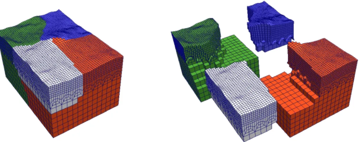
We have selected a study volume of 150x150x40 km3 where the Alto Tiberina and Gubbio fault zones are located (Figure 33). We have defined the geometry by means of Rhinoceros (http://www.rhino3d.com, a graphic vector code for tridimensional objects). The surface topography is resampled at 1 km from Shuttle Radar Topographic Mission (SRTM, http://www2.jpl.nasa.gov/srtm/; Figure 34). We have built fault blocks including the ATF and GF zones (Figure 34) with thickness of 800
m. The GF and ATF geometry follow the works of Mirabella et al (2004) and Mirabella et al (2011) respectively. These fault blocks have been imprinted in the crustal block through Boolean operators. Figure 34b show the obtained geometry (ATF_nonplanar model). Since we aim to explore the impact of the fault roughness, we have prepared a second crustal block where a planar ATF zone is considered (ATF_planar model; Figure 34a).
Fig. 34. Geometry for ATF_planar model a) and ATF_nonplanar model b). We build a crustal volume
We have imported the obtained geometries in Cubit (https://cubit.sandia.gov) to build the tetrahedral mesh (Figure 35). This element type increased the computational costs respect to hexahedra but is better suited to low angle geometries (as the ATF).
Rheology, material properties and boundary conditions are defined in PyLith (http://geodynamics.org/cig/software/pylith/; Chapter 3). The crust is characterised entirely by an elastic rheology defined in table 6. We consider an ATF locking depth of 5 km for both the models. As for the 2D models, in an initial stage the crust is subjected to gravity load and then stretched for 1000 years. According to the present-day plate kinematics of the Northern Apennines region, we apply a constant horizontal velocity of 0.5 mm/yr and 3.5 mm/yr on the SW and NE lateral boundaries respectively (Figure 35).
Fig. 35. Mesh and boundary conditions for ATF_planar and ATF_nonplanar models. Note that the
Young modulus (Pa) Poissons ratio Density (Kg/m3)
Intact rock 5.33e10 0.25 2570
ATF fault zone 1e7 0.35 2500
Gubbio fault zone 1e8 0.35 2500
Tab. 6. Elastic properties for ATF_planar and ATF_nonplanar models.
5.3. Model results
In Figure 36 we compare the velocity field obtained from the modelling with the observed GPS data. We can note that both the models (ATF_planar and ATF_nonplanar) agree with the general velocity field observed. The fitting is well constrained both for the velocity vector orientations that for the magnitude. The difference between ATF_planar and ATF_nonplanar models can be observed in Figure 37 where horizontal velocity profiles are plotted along the same cross section used for the 2D models. The models show approximately the same trend of the horizontal velocity. A very small decreasing of the ATF_nonplanar respect to ATF_planar model is observed.
Figure 38 shows the interseismic stress build-up for ATF_planar and ATF_nonplanar models. Here, larger differences between the models are found. Considering the ATF_planar case (Figure 38a) we observe that the stress build-up is mainly located above 5 km of depth and along the Gubbio fault. Below the ATF locking depth the stress build-up decreases and it is homogeneous for the entire fault. Only local stress anomalies (with relative higher stress values) are found near 12 km of depth where there is an abrupt change of dip between ATF-ramp and ATF-flat. Otherwise in the
ATF_nonplanar model (Figure 38b) the stress distribution is strongly affected by the ATF roughness both above that below the ATF locking depth. In particular we can observe that below 5 km of depth strong stress accumulations are located along the ATF ramp due to the roughness slopes.
Fig. 36. Comparison between the observed and modelled velocity field. Note that the differences
between ATF_planar (a) and ATF_nonplanar (b) models are minimal. The dotted lines indicate the range of GPS stations considered in figure 37.
Fig. 37. Horizzontal velocity obtained by ATF_planar and ATF nonplanar models. In order to compare
the velocity field obtained with the 2D models, we consider only the GPS stations whose distance from the cross-section is less then 10 km (the limit is represented by the dotted line in figure 36); in particular the GPS stations considered are from SW to NE: SIO1, REPI, CSSB, VALC, UMBE, ATLO, MVAL, PIET, ATFO, ATBU, FOSS.
5.4. Discussion and concluding remarks
The ATF_planar model results are in good agreement with the ATF_nonplanar case at least in some aspects. In fact, if the horizontal velocity profiles (Figure 37) show similar trends, the stress distribution is strongly affected by the ATF roughness in the ATF_nonplanar model (Figure 38). These models highlight that the stress build-up is mainly located in the first 5 km of depth along the Gubbio antithetic fault, that being well-oriented with σ1, could fail seismically. At same time, overstressed patches induced by the geometrical irregularity of the ATF zone, could also fail seismically, if
well oriented with σ1. In this case, the microseismicity situated below 5 km of depth could be justified (Chapter 2).
Fig. 38. Interseismic stress build-up for ATF_planar (a) and ATF_nonplanar (b) models. Note that, in
the both cases, the stress is mainly accumulated in the first 5 km of depth and along the Gubbio fault zone. In the ATF_nonplanar model the stress distribution is affected by the ATF roughness, in fact high values of stress below 5 km are found.
In this context the dip-angle variation of the fault plane assumes an important role respect to the frictional reactivation theory described in the chapter 2. In figure 39a we plot the ATF the dip-angle variation on the geometry by Mirabella et al., (2011). We can observe that the dip-angle distribution is strongly heterogeneous though the main dip is around 17°. In fact some very flat areas (1°) coexist with higher dip area (greater then 35°). Considering the analysis on the frictional reactivation of a normal fault done in the chapter 2, we calculate the distribution of the maximum frictional coefficient µ (Figure 39b) for which it is possible to obtain slip along the dip-angle distribution of figure 39a. In other words, initially, we calculate the reactivation angle 2θ* (90-dip) for frictional lock-up (R→∞) and after we calculate the correspondent frictional coefficient µ (values of 2θ* corresponding to different values of µ are plotted in Figure 40). Figure 39b shows that the frictional reactivation of the Alto Tiberina low angle normal fault is possible along some patches even considering typical Byrlee friction coefficient (in this case 0.6-0.75) and without to invoke necessarily fluid overpressure. Then, these patches are surrounding by a matrix defined by low values of friction (µ<0.4). Rocks with high values of friction (µ>0.6) found along exhumed low-angle normal faults highlight a prevalent velocity weakening behaviour while for low values of µ (<0.4) they point out a velocity strengthening behaviour (Collettini, 2011). This indicate that the microseismicty on the ATF plane could be induced on patches with high values of µ, overstressed by the stable slip promoted by velocity strengthening material.
Fig. 39. a) ATF dip-angle variation depending of the roughness in degree. b) Maximum friction