2020-04-18T10:36:28Z
Acceptance in OA@INAF
The ASKAP/EMU Source Finding Data Challenge
Title
Hopkins, A. M.; Whiting, M. T.; Seymour, N.; Chow, K. E.; Norris, R. P.; et al.
Authors
10.1017/pasa.2015.37
DOI
http://hdl.handle.net/20.500.12386/24102
Handle
PUBLICATIONS OF THE ASTRONOMICAL SOCIETY OF AUSTRALIA
Journal
32
Number
arXiv:1509.03931v1 [astro-ph.IM] 14 Sep 2015
doi: 10.1017/pas.2018.xxx.
The ASKAP/EMU Source Finding Data Challenge
A. M. Hopkins1,∗, M. T. Whiting2, N. Seymour3, K. E. Chow2, R. P. Norris2, L. Bonavera4, R. Breton5, D. Carbone6, C. Ferrari7, T. M. O. Franzen3, H. Garsden8, J. Gonz´alez-Nuevo9,4, C. A. Hales10,11, P. J.
Hancock3,12,13, G. Heald14,15, D. Herranz4, M. Huynh16, R. J. Jurek2, M. L´opez-Caniego17,4, M. Massardi18, N. Mohan19, S. Molinari20, E. Orr`u14, R. Paladino21,18, M. Pestalozzi20, R. Pizzo14, D. Rafferty22, H. J. A. R¨ottgering23, L. Rudnick24, E. Schisano20, A. Shulevski14,15, J. Swinbank25,6, R. Taylor26,27, A. J. van der Horst28,6
1 Australian Astronomical Observatory, PO Box 915, North Ryde, NSW, 1670, Australia 2 CSIRO Astronomy & Space Science, PO Box 76, Epping, NSW 1710, Australia
3 International Centre for Radio Astronomy Research, Curtin University, GPO Box U1987, Perth WA 6845, Australia 4 Instituto de F´ısica de Cantabria (CSIC-UC), Santander, 39005 Spain
5 Jodrell Bank Centre for Astrophysics, The University of Manchester, Manchester, M13 9PL, UK
6 Anton Pannekoek Institute for Astronomy, University of Amsterdam, Postbus 94249, 1090 GE Amsterdam, The Netherlands 7 Laboratoire Lagrange, Universit´e Cˆote d’Azur, Observatoire de la Cˆote d’Azur, CNRS, Blvd de l’Observatoire, CS 34229, 06304
Nice cedex 4, France
8 Laboratoire AIM (UMR 7158), CEA/DSM-CNRS-Universit´e Paris Diderot, IRFU, SEDI-SAP, Service dAstrophysique, Centre de
Saclay, F-91191 Gif-Sur-Yvette cedex, France
9 Departamento de F´ısica, Universidad de Oviedo, C. Calvo Sotelo s/n, 33007 Oviedo, Spain
10National Radio Astronomical Observatory, P.O. Box O, 1003 Lopezville Road, Socorro, NM 87801-0387, USA 11Jansky Fellow, National Radio Astronomical Observatory
12Sydney Institute for Astronomy, School of Physics A29, The University of Sydney, NSW 2006, Australia 13ARC Centre of Excellence for All-Sky Astrophysics (CAASTRO)
14ASTRON, the Netherlands Institute for Radio Astronomy, Postbus 2, 7990 AA, Dwingeloo, The Netherlands 15University of Groningen, Kapteyn Astronomical Institute, Landleven 12, 9747 AD Groningen, The Netherlands
16International Centre for Radio Astronomy Research, M468, University of Western Australia, Crawley, WA 6009, Australia 17European Space Agency, ESAC, Planck Science Office, Camino bajo del Castillo, s/n, Urbanizaci´on Villafranca del Castillo,
Villanueva de la Ca˜nada, Madrid, Spain
18INAF-Istituto di Radioastronomia, via Gobetti 101, 40129 Bologna, Italy
19National Centre for Radio Astrophysics, Tata Institute of Fundamental Research, Post Bag 3, Ganeshkhind, Pune 411 007, India 20IAPS - INAF, via del Fosso del Cavaliere 100, I - 00173 Roma, Italy
21Department of Physics and Astronomy, University of Bologna, V.le Berti Pichat 6/2, 40127 Bologna, Italy 22Hamburger Sternwarte, Universit¨at Hamburg, Gojenbergsweg 112, D-21029 Hamburg, Germany
23Leiden Observatory, Leiden University, P.O. Box 9513, 2300 RA, The Netherlands
24Minnesota Institute for Astrophysics, University of Minnesota, 116 Church St. SE, Minneapolis, MN 55455 25Department of Astrophysical Sciences, Princeton University, Princeton, NJ 08544, USA
26Department of Astronomy, University of Cape Town, Private Bag X3, Rondebosch, 7701, South Africa 27Department of Physics, University of the Western Cape, Robert Sobukwe Road, Bellville, 7535, South Africa 28Department of Physics, The George Washington University, 725 21st Street NW, Washington, DC 20052, USA
Abstract
The Evolutionary Map of the Universe (EMU) is a proposed radio continuum survey of the Southern
Hemisphere up to declination +30◦, with the Australian Square Kilometre Array Pathfinder (ASKAP). EMU
will use an automated source identification and measurement approach that is demonstrably optimal, to maximise the reliability, utility and robustness of the resulting radio source catalogues. As part of the process of achieving this aim, a “Data Challenge” has been conducted, providing international teams the opportunity to test a variety of source finders on a set of simulated images. The aim is to quantify the accuracy of existing automated source finding and measurement approaches, and to identify potential limitations. The Challenge attracted nine independent teams, who tested eleven different source finding tools. In addition, the Challenge initiators also tested the current ASKAPsoft source-finding tool to establish how it could benefit from incorporating successful features of the other tools. Here we present the results of the Data Challenge, identifying the successes and limitations for this broad variety of the current generation of radio source finding tools. As expected, most finders demonstrate completeness levels close to 100% at ≈ 10 σ dropping to levels around 10% by ≈ 5 σ. The reliability is typically close to 100% at ≈ 10 σ, with performance to lower sensitivities varying greatly between finders. All finders demonstrate the usual trade-off between completeness and reliability, whereby maintaining a high completeness at low signal-to-noise comes at the expense of reduced reliability, and vice-versa. We conclude with a series of recommendations for improving the performance of the ASKAPsoft source-finding tool.
1 INTRODUCTION
Measuring the properties of astronomical sources in im-ages produced by radio interferometers has been suc-cessfully achieved for many decades through a vari-ety of techniques. Probably the most common in re-cent years has been through identifying local peaks of emission above some threshold, and fitting two-dimen-sional Gaussians (e.g., Condon 1997). This approach is in principle substantially unchanged from the very ear-liest generation of automated source detection and mea-surement approaches in radio interferometric imaging. These also used a thresholding step followed by integra-tion of the flux density in peaks of emission above that threshold (e.g., Kenderdine et al. 1966). This in turn followed naturally from the earlier practice of defining a smooth curve through the minima of paper trace pro-files to represent the background level (e.g., Large et al. 1961).
A variety of automated tools for implementing this approach have been developed. In almost all cases the automatically determined source list requires some level of subsequent manual adjustment to eliminate spuri-ous detections or to include objects deemed to be real but that were overlooked by the automated finder. This manual adjustment step, again, has remained un-changed since the earliest days of radio source measure-ment (e.g., Hill & Mills 1962).
As radio surveys have become deeper and wider, and the numbers of sources in the automated cata-logues becomes large, such manual intervention is pro-gressively less feasible. The FIRST survey (White et al. 1997) contains about 900 000 sources, and the NVSS (Condon et al. 1998) about 1.8 million sources. In the case of future wide-area and deep surveys with new tele-scope facilities, such as the Australian Square Kilometre Array Pathfinder (ASKAP, Johnston et al. 2007), this number will be increased by substantially more than an order of magnitude. The Evolutionary Map of the Universe (EMU, Norris et al. 2011), for example, is ex-pected to yield about 70 million radio sources. The full Square Kilometre Array will produce orders of magni-tude more again (e.g., Hopkins et al. 2000).
There has been a strong movement in recent years to ensure that the automated source detection pipelines implemented for these next generation facilities pro-duce catalogues with a high degree of completeness and reliability, together with well-defined and char-acterised measurement accuracy. Several recent anal-yses explore the properties of various source-finders, and propose refinements or developments to such tools (e.g., Popping et al. 2012; Huynh et al. 2012; Hales et al. 2012; Hancock et al. 2012; Mooley et al. 2013; Peracaula et al. 2015). At the second annual SKA
∗Email: [email protected]
Pathfinder Radio Continuum Surveys (SPARCS) work-shop, held in Sydney over 2012 May 30 to 2012 June 1, many of these results were presented and discussed. A consensus was reached that a blind source finding challenge would be a valuable addition to our current approaches for understanding the strengths and limita-tions of the many source-finding tools and techniques presently available. The Data Challenge presented here was initiated as a result. The intended audience for this work includes not only the ASKAP team working on source finding solutions, but also the developers of as-tronomical source finding and related tools, and poten-tial coordinators of future Data Challenges. The out-comes of this work have applicability to all these areas. The goal of the Data Challenge is to assess the completeness, reliability, accuracy, and common failure modes, for a variety of source-finding tools. These statis-tics and outcomes are presented below for all the tools tested in the Challenge. The outcomes are being used to directly inform developments within the ASKAP source finding pipeline. The primary focus is on ensuring that the ASKAP source finder is as robust as possible for producing the EMU source catalogue, although these results are clearly of broad utility, in particular for many of the current SKA Pathfinders and surveys.
The scope of the current Challenge is limited inten-tionally to point-sources or point-like sources (sources only marginally extended), due to the inherent dif-ficulty faced by automated source finders in dealing with complex source structure. We do test the perfor-mance of such finders on somewhat extended sources in our analysis, although given this limitation we do not explore such performance in great detail. This is clearly an area that deserves more explicit attention, with a focus on how to develop automated source find-ers that accurately characterise extended source struc-ture (e.g., Hollitt & Johnston-Hollitt 2012; Frean et al., 2014). Even with this limitation, there is clearly still much that can be learned about the approach to au-tomating a highly complete and reliable point source detection tool. It is hoped that future Data Challenges will follow from this initial effort, exploring more com-plex source structures, as well as innovative approaches to the source detection and characterisation problem.
Below we describe the Data Challenge itself (§ 2) and the construction of the artificial images used (§ 3). This is followed by our analysis of the performance of the submitted finders (§ 4) and a discussion comparing these results (§ 5). We conclude in § 6 with a summary of the outcomes.
2 THE DATA CHALLENGE
The Data Challenge originators (Hopkins, Whiting and Seymour) had responsibility for preparing the artificial source lists and images for the Challenge, initiating and PASA (2018)
promoting it to potential participants and coordinat-ing the Challenge itself, as well as the primary analysis of the outcomes. The Data Challenge required teams to register their participation by 2012 November 30. Three artificial images were provided, along with a selection of ancillary data detailed below. The deadline for sub-mitting the three source lists for each registered source finder was 2013 January 15.
Participating teams were instructed to provide de-tails of the source finding tool being tested, including the name, version number if appropriate, instructions for obtaining the tool itself, and any other information to uniquely identify the tool and mode or parameters of operation as relevant. The teams were also required to identify any potential conflicts of interest that may have biased or influenced their analysis, or prevented the analysis from being truly blind. No such conflicts were identified by any participating teams.
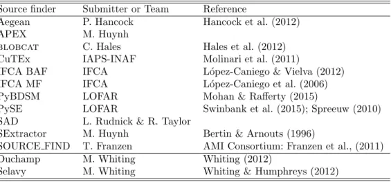
The source lists submitted by the teams were required to have file names allowing them to be uniquely as-sociated with the corresponding Challenge image. The format of each source list was required to be a sim-ple ascii text file containing one line per source, with a header line (or lines) marked by a hash (#) as the initial character, to uniquely define the columns of the ascii table. The columns were required to include RA and Dec, peak and integrated flux density, deconvolved semi-major axis, deconvolved semi-minor axis, and posi-tion angle. Errors on all of these quantities were also re-quested. Multiple submissions were acceptable if teams desired to have different operating modes or parameter sets for a given tool included in the analysis. Several of the submitted finders included multiple different modes or parameter settings, and these are referred to in the text and figures below by the name of the finder fol-lowed by the mode of use in brackets. Not all submis-sions included size and position angle measurements, as not all tools tested necessarily provide those measure-ments. The list of tools submitted, with published ref-erences to the tool where available, is given in Table 1. A brief description of each finder and how it was used in the Challenge is presented in Appendix A. We note that some finders may need considerable fine tuning of parameters and consequently the conclusions presented from this Challenge reflect the particular finder imple-mentation used for these tests.
In addition to the tools submitted by participants, two additional tools were tested by the Challenge origi-nators. These are Duchamp and Selavy, tools that were both authored by Whiting, and multiple modes for these finders were tested. While all care has been taken to treat these tools and their outputs objectively, we ac-knowledge the conflict of interest present, and these cannot be assessed in a truly “blind” fashion as with the other tools tested. Bearing this in mind, we felt that it would be valuable to identify the strengths and
weaknesses of these tools in the same way as the others that are being tested in a truly “blind” fashion. The in-tent is to identify elements of the best-performing tools that can subsequently be incorporated into the ASKAP source finder, or common failure modes that can be eliminated if present. Note that Selavy is the current prototype for the ASKAP pipeline-based source-finder.
3 ARTIFICIAL IMAGE CREATION 3.1 Artificial source catalogues
For the Data Challenge images we created three input catalogues:
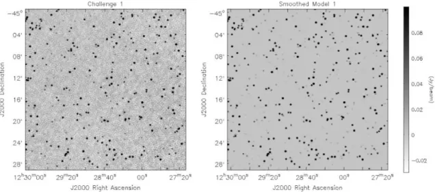
1. A bright source catalogue (Figure 1). The purpose of this test was to obtain an initial comparison of the different methods and to search for subtle systematic effects. We were interested in assess-ing the performance of source finders in a non-physical scenario to aid in determining whether there were any aspects of the real sky that in-fluenced the outcomes in subtle ways. We cre-ated a catalogue with a surface density of about 3800 sources per square degree (the image syn-thesised beam size is ≈ 11′′, details in § 3.2) with a uniform distribution in logarithmic flux den-sity spanning 0.2 < S1.4GHz(mJy)< 1000. The po-sitions were randomly assigned, with RA and Dec values for each source having a uniform chance of falling anywhere within the field.
2. A fainter catalogue with pseudo-realistic cluster-ing and source counts (Figure 2). Here we used a surface density of about 800 sources per square degree (the image synthesised beam size is ≈ 11′′, details in § 3.2) and had an increasing num-ber of faint sources as measured in bins of log-arithmic flux density, to mimic the real source counts (e.g., Hopkins et al. 2003; Norris et al. 2011). Sources were assigned flux densities in the range 0.04 < S1.4GHz(mJy)< 1000. The distribu-tion of source posidistribu-tions was designed to roughly correspond to the clustering distributions mea-sured by Blake & Wall (2002) for sources having S1.4GHz > 1 mJy, and to Oliver et al. (2004) for S1.4GHz < 1 mJy. In the latter case we assume that faint radio sources have similar clustering to faint IRAC sources, in the absence of explicit cluster-ing measurements for the faint population, and on the basis that both predominantly reflect a chang-ing proportion of low luminosity AGN and star forming galaxy populations. In each case we be-gan with an initial random list of source locations, then used an iterative process to test the cluster-ing signal in the vicinity of each source, relocatcluster-ing
Figure 1.A subsection of the first Data Challenge image (left), and the input source distribution to this image (right). This image includes sources distributed randomly with a flux density distribution that is uniform in the logarithm of flux density. This distribution gives rise to a much higher surface density of bright sources, and proportionally more bright sources compared to faint sources, than in the real sky.
Figure 2.A subsection of the second Data Challenge image (left), and the input source distribution to this image (right). This image includes sources distributed with intrinsic clustering, and with a flux density distribution drawn from the observed source counts (e.g., Hopkins et al. 2003), in an effort to mimic the characteristics of the real sky.
neighbour sources until the desired clustering was reproduced.
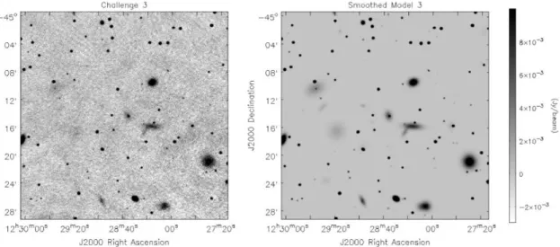
3. The same as (2), but with some sources extended (Figure 3). We randomly designated 20% of those sources to be elliptical Gaussians with the to-tal flux conserved (and therefore having a lower peak flux density). These elliptical Gaussians were assigned major axis lengths of 5′′ to 140′′, with brighter sources likely to be more extended than fainter ones. The minor axis length was then
ran-domly varied between 30% and 100% of the major axis length.
In Figures 1-3 we show subsections of the Challenge images used and the input source models, in order to illustrate cleanly the characteristics of the noise in the images. The input sources were assigned to have flat spectra (α = 0, where Sν∝ να) as investigations of spectral index effects are beyond the scope of these tests. For all three Challenges, the distribution of source flux densities end up spanning a broad range of signal-PASA (2018)
Figure 3.A subsection of the third Data Challenge image (left), and the input source distribution to this image (right). This image includes sources as for the second Data Challenge image, but with 20% of the sources now assigned a non-negligible physical extent. The extended sources are modelled as two-dimensional elliptical Gaussians.
10-3 10-2 10-1 100 101 102 103 104 S1.4 (mJy) 0 500 1000 1500 2000 2500 3000 3500 4000 N Challenge 1 Challenge 2 Challenge 3
Figure 4.The distribution of input source flux densities for the three Challenges.
to-noise (S/N), from S/N< 1 to S/N> 100 (Figure 4). Each catalogue covered a square region of 30 deg2 (to match the ASKAP field-of-view) and were centred ar-bitrarily at RA= 12h30m, Dec= −45◦.
3.2 Artificial image generation
The images were created with two arcsecond pixels. To simplify the computational elements of the imaging each source was shifted slightly to be at the centre of a pixel. If multiple sources were shifted to a common location they were simply combined into a single input source by summing their flux densities. This step had a negligi-ble effect on both the implied clustering of the sources and the input flux density distribution, but a
signifi-cant reduction in the computational requirements for producing the artificial images. The input source cata-logue used subsequently to assess the performance of the submitted finders was that produced after these loca-tion shifting and (if needed) flux combining steps. Sim-ulating a more realistic distribution of source positions should be explored in future work to assess the effect on finder performance for sources lying at pixel corners rather than pixel centres.
The image creation step involves mimicking the pro-cess of observation, populating the uv plane by sampling the artificial noise-free sky for a simulated 12 hour syn-thesis with the nominal 36 ASKAP antennas, adding realistic noise (assuming Tsys= 50K and aperture ef-ficiency η = 0.8) to the visibilities. Noise was added in the uv plane in the XX and YY polarisations with no cross-polarisation terms. This simulates the thermal noise in the visibilities in order to correctly mimic the behaviour of the real telescope. The image-plane noise consequently incorporates the expected correlation over the scale of the restoring beam. Because of a limitation in computing resources, a reduced image size compared to that produced by ASKAP was simulated giving a field of view of 15.8 deg2 (or 11.6 deg2 once cropped, described further below), as it was judged this was suf-ficient to provide a large number of sources yet still keep the images of a manageable size for processing purposes. The visibilities were then imaged via Fourier transfor-mation and deconvolution. The deconvolution step was run for a fixed number of iterations for each of the three Challenge images. As a consequence of this step, limited by available CPU time for this compute-intensive pro-cess, the image noise level in the simulations is signifi-cantly higher than the nominal theoretical noise. This is
exacerbated by the presence of many faint sources below the measured noise level in the simulated images. We emphasise that the processing of real ASKAP images will not be limited in this way. For Challenge 1 the noise level was higher, by almost a factor of 10, than in the im-ages for Challenges 2 and 3. We attribute this, and the subsequent low dynamic range in the flux-density distri-bution of sources able to be measured in Challenge 1, to the non-physical distribution of flux densities resulting from the high surface density of bright sources.
Due to the density of sources on the sky, especially for Challenge 1, and with clustering (random or not) many sources were close enough together that they were ei-ther assigned to the same pixel, or would fall within the final restored beam of the image (11.2′′× 10.7′′, PA= 3.1◦) of an adjacent source. While sources with their peaks lying within the same resolution element may be able to be distinguished, given sufficient S/N de-pending on the separation, the bulk of measured radio sources in large surveys are at low S/N. Even sources in this regime with their peaks separated by more than one resolution element but still close enough to overlap are clearly a challenge (Hancock et al. 2012), even without adding the extra complexity of sources lying within a common resolution element. To avoid making the Data Challenge too sophisticated initially and to focus on the most common issues, for Challenges 1 and 2 all sources from the preliminary input catalogue that lay within 11′′ of each other were replaced by a single source de-fined as the combination of the preliminary sources by adding their fluxes and using the flux weighted mean positions. While most of these matches were pairs we also accounted for the small number of multiple such matches.
For Challenge 3 with 20% of the sources potentially quite extended we had to employ a different method. For relatively compact sources, defined as those having a major axis < 16.8′′(1.5×FWHM), we combined them as before if they were isolated from extended sources. For the rest of the sources with larger extent we simply flagged them as either being isolated if no other sources overlapped the elliptical Gaussian, or as being blended. For comparison with the submitted catalogues, we restricted both the simulated and measured catalogues to areas that had good sensitivity, removing the edges of the image where the image noise increased. In practice, we applied a cutoff where the theoretical noise increased by a factor of 2.35 over the best (lowest) noise level in the field.
4 ANALYSIS
4.1 Completeness and reliability
Completeness and reliability are commonly used statis-tics for a measured set of sources to assess the
per-formance of the source finder. The completeness is the fraction of real (input) sources correctly identified by the measurements, and the reliability is the fraction of the measured sources that are real.
To compare the submitted results for each finder with the input source lists, we first perform a simple posi-tional cross-match. For Challenges 1 and 2 we define a measured source to be a match with an input source if it is the closest counterpart with a positional offset less than 5′′. This offset corresponds to 2.5 pixels or about 0.5×FWHM of the resolution element, so is a suitably small offset to minimise false associations. By construction there are no input sources within this po-sitional offset of each other, ensuring that any match with a measured source should be a correct association. For Challenge 3, given the presence of extended sources, we increased the offset limit to 30′′, roughly 3×FWHM of the resolution element, to account for greater posi-tional uncertainties in the detected sources by the differ-ent finders. This does lead to the possibility of spurious cross-matches between measured and input sources. We do not attempt to account for this effect in the current analysis, though, merely noting that this is a limita-tion on the accuracy of these metrics for Challenge 3, and that any systematics are likely to affect the differ-ent finders equally. We avoid using additional criteria such as flux density (e.g., Wang et al. 2014) to refine the cross-matching, as this has the potential to conflate our analyses of positional and flux density accuracy. Us-ing this definition, we calculate the completeness and reliability of the input catalogues for each of the three Challenges. These are shown in Figures 5, 6 and 7.
We show these measurements as a function of the in-put source flux density for the completeness measure and of the measured source flux density for the reliabil-ity. Ideally, the S/N rather than the flux density should be used here, but because of the way the artificial im-ages have been generated, following a simulated obser-vation and deconvolution process, the intrinsic S/N is not known a priori. We measure the root-mean-square (rms) noise level in the images directly, at several rep-resentative locations selected to avoid bright sources. We note that the unit of flux density in each pixel is mJy/beam, so that changing the pixel scale in the im-age changes only the number of pixels/beam, not the flux scaling. We measure σ ≈ 9 mJy for Challenge 1 and σ ≈ 1 mJy for each of Challenge 2 and 3, although the value fluctuates as a function of location in the image by up to ±2 mJy for Challenge 1 and ±0.5 mJy for Chal-lenges 2 and 3. Bearing these details in mind, much of the discussion below refers in general terms to S/N rather than to flux density, in order to facilitate com-parisons between the Challenges.
The completeness and reliability curves give insights into the performance of the various finders. In broad terms, most finders perform well at high S/N, with de-PASA (2018)
0.0 0.5 1.0 Aegean Apex Blobcat 0.0 0.5 1.0 CuTEx Duchamp (atrous) Duchamp (basic) 0.0 0.5 1.0 Duchamp (smooth) IFCA (BAF) IFCA (MF) 0.0 0.5 1.0
Co
mp
let
en
ess
PyBDSM (Gaussians)PyBDSM (sources)PySE (D5A3) 0.0 0.5 1.0 PySE (FDR) SAD Selavy (atrous) 0.0 0.5 1.0 Selavy (basic) Selavy (box) Selavy (smooth) 0.0 0.5 1.0 Selavy (weight) SExtractor (10 beam) SExtractor (30 beam) 102 103 S1.4 (mJy) 0.0 0.5 1.0 SOURCE_FIND 0.0 0.5 1.0 Aegean Apex Blobcat 0.0 0.5 1.0 CuTEx Duchamp (atrous) Duchamp (basic) 0.0 0.5 1.0 Duchamp (smooth) IFCA (BAF) IFCA (MF) 0.0 0.5 1.0
Re
lia
bil
ity
PyBDSM (Gaussians)PyBDSM (sources)PySE (D5A3)0.0 0.5 1.0 PySE (FDR) SAD Selavy (atrous) 0.0 0.5 1.0 Selavy (basic) Selavy (box) Selavy (smooth) 0.0 0.5 1.0 Selavy (weight) SExtractor (10 beam) SExtractor (30 beam) 102 103 S1.4 (mJy) 0.0 0.5 1.0 SOURCE_FIND
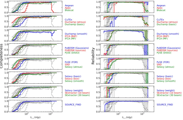
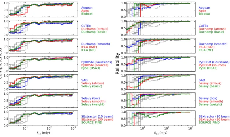
Figure 5.The completeness and reliability fractions (left and right respectively) as a function of input source flux density (completeness) or measured source flux density (reliability) for each of the tested source finders for Challenge 1. The grey lines show the distribution for all finders in each panel, to aid comparison for any given finder.
clining completeness and reliability below about 10 σ. In general we see the expected trade-off between complete-ness and reliability, with one being maintained at the expense of the other, but there are clearly variations of performance between finders and Challenges. It may be desirable in some circumstances to use certain metrics (such as the S/N at which completeness drops to 50%, or the integrated reliability above some threshold) to summarise the information contained in the complete-ness and reliability distributions. Due to the nature of the current investigation, though, and in order not to obscure any subtle effects, we have chosen to focus on the properties of the full distributions.
For all finders, the qualitative performance in Chlenge 1 is similar to the performance in ChalChlenge 2, al-though quantitatively the completeness and reliability are poorer in Challenge 1 than in Challenge 2. Find-ers that demonstrate a good performance at low S/N in terms of completeness while also maintaining high reliability include Aegean, blobcat, SExtractor and
SOURCE FIND. IFCA (in both modes) has a very high completeness, but at the expense of reliability. CuTEx shows the lowest completeness as well as reliability at faint levels.
Some finders (blobcat, Duchamp, and Selavy in smooth mode) at high S/N show dips or declining per-formance in either or both of completeness and relia-bility, where the results should be uniformly good. At very high S/N we expect 100% completeness and relia-bility from all finders. Some finders that perform well in terms of completeness still show poorer than expected levels of reliability. Selavy in most modes falls into this category, as does PyBDSM (Gaussians) for Challenge 2 (but not Challenge 1, surprisingly).
For those finders that otherwise perform well by these metrics, we can make a few more observations. First it is clear that the APEX finder used a higher threshold than most finders, approximately a 10 σ threshold com-pared to something closer to 5 σ for all others. Is it also apparent that SAD demonstrates a drop in reliability
0.0 0.5 1.0 Aegean Apex Blobcat 0.0 0.5 1.0 CuTEx Duchamp (atrous) Duchamp (basic) 0.0 0.5 1.0 Duchamp (smooth) IFCA (BAF) IFCA (MF) 0.0 0.5 1.0
Co
mp
let
en
ess
PyBDSM (Gaussians)PyBDSM (sources)PySE (D5A3) 0.0 0.5 1.0 PySE (FDR) SAD Selavy (atrous) 0.0 0.5 1.0 Selavy (basic) Selavy (box) Selavy (smooth) 0.0 0.5 1.0 Selavy (weight) SExtractor (10 beam) SExtractor (30 beam) 101 102 103 S1.4 (mJy) 0.0 0.5 1.0 SOURCE_FIND 0.0 0.5 1.0 Aegean Apex Blobcat 0.0 0.5 1.0 CuTEx Duchamp (atrous) Duchamp (basic) 0.0 0.5 1.0 Duchamp (smooth) IFCA (BAF) IFCA (MF) 0.0 0.5 1.0
Re
lia
bil
ity
PyBDSM (Gaussians)PyBDSM (sources)PySE (D5A3)0.0 0.5 1.0 PySE (FDR) SAD Selavy (atrous) 0.0 0.5 1.0 Selavy (basic) Selavy (box) Selavy (smooth) 0.0 0.5 1.0 Selavy (weight) SExtractor (10 beam) SExtractor (30 beam) 101 102 103 S1.4 (mJy) 0.0 0.5 1.0 SOURCE_FIND
Figure 6.The completeness and reliability fractions (left and right respectively) as a function of input source flux density (completeness) or measured source flux density (reliability) for each of the tested finders for Challenge 2. The grey lines show the distribution for all finders in each panel, to aid comparison for any given finder.
below about 10 σ that declines faster than most of the other similarly-performing finders, before recovering at the lowest S/N at the expense of completeness. This is emphasised more in Challenge 1 than in Challenge 2.
The performance of most finders in Challenge 3 is similar to that in other Challenges, except for a reduced completeness and reliability. This is not surprising as the 20% of sources that are extended will have a re-duced surface brightness and hence peak flux density compared to their total flux density, so many of the ex-tended sources are below the threshold for detection for all the finders tested. In addition, the reliability is likely to be reduced at low to modest S/N as a consequence of the extended emission from these sources pushing some noise peaks above the detection threshold. This may also arise from the number of artifacts related to the extended sources that are visible in Figure 3. Most finders still demonstrate a completeness for Challenge 3 of better than around 80% above reasonable flux den-sity (or S/N) thresholds (e.g., S/N≥ 8 − 10), which is
encouraging since this is the fraction of input sources in Challenge 3 that are point sources. Despite this, blob-cat, PyBDSM (sources), PySE (D5A3), SAD and SEx-tractor maintain very high reliability in their measured sources for Challenge 3. Other finders, though, includ-ing Aegean and SOURCE FIND, as well as Selavy, show very low reliability in this Challenge, even at very high S/N, suggesting that there may be additional issues con-tributing to detection of false sources in the presence of extended sources. We note that these finders are de-signed for the detection of point sources, but further investigation is needed to establish why the presence of extended emission affects their performance in this way. One possibility is that an extended source may be broken into a number of individual point-source com-ponents, due to noise fluctuations appearing as local maxima. These would then appear as false detections since they do not match up to an input source.
Since maximising both completeness and reliability is one clear goal of source finding, we illustrate in Fig-PASA (2018)
0.0 0.5 1.0 Aegean Apex Blobcat 0.0 0.5 1.0 CuTEx Duchamp (atrous) Duchamp (basic) 0.0 0.5 1.0 Duchamp (smooth) IFCA (BAF) IFCA (MF) 0.0 0.5 1.0
Co
mp
let
en
ess
PyBDSM (Gaussians) PyBDSM (sources) PySE (D5A3) 0.0 0.5 1.0 SAD Selavy (atrous) Selavy (basic) 0.0 0.5 1.0 Selavy (box) Selavy (smooth) Selavy (weight) 101 102 103 S1.4 (mJy) 0.0 0.5 1.0 SExtractor (10 beam) SExtractor (30 beam) SOURCE_FIND 0.0 0.5 1.0 Aegean Apex Blobcat 0.0 0.5 1.0 CuTEx Duchamp (atrous) Duchamp (basic) 0.0 0.5 1.0 Duchamp (smooth) IFCA (BAF) IFCA (MF) 0.0 0.5 1.0Re
lia
bil
ity
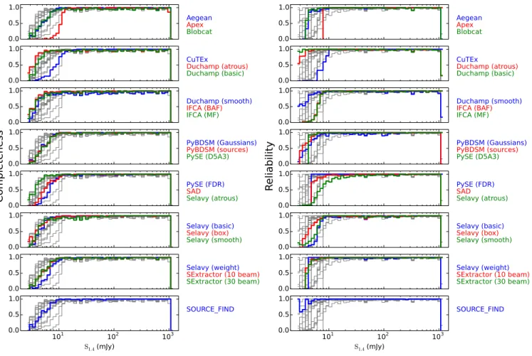
PyBDSM (Gaussians) PyBDSM (sources) PySE (D5A3) 0.0 0.5 1.0 SAD Selavy (atrous) Selavy (basic) 0.0 0.5 1.0 Selavy (box) Selavy (smooth) Selavy (weight) 101 102 103 S1.4 (mJy) 0.0 0.5 1.0 SExtractor (10 beam) SExtractor (30 beam) SOURCE_FINDFigure 7.The completeness and reliability fractions (left and right respectively) as a function of input source flux density (completeness) or measured source flux density (reliability) for each of the tested finders for Challenge 3. The grey lines show the distribution for all finders in each panel, to aid comparison for any given finder. Note that PySE (FDR) was only submitted for Challenges 1 and 2, and does not appear here.
ure 8 how the product of completeness and reliability for all finders varies as a function of the input source flux density for each of the three Challenges. The ad-vantage of this metric is that it retains the dependence on flux density (or S/N), so that the joint performance can be assessed as a function of source brightness. This may serve to provide a more direct or intuitive com-parison between finders at a glance than the separate relationships from Figures 5, 6 and 7. It readily high-lights finders than perform poorly at high S/N (e.g., blobcatand Duchamp in Challenge 1), and the range of performance at low S/N. It also highlights that most finders follow a quite tight locus in this product as the flux density drops from about 10 σ to 5 σ and below, and can be used to identify those that perform better or worse than this typical level. Clearly, though, the ori-gin of any shortfall in the product of the two statistics needs to be identified in the earlier Figures.
There is an issue related to source blending that af-fects the degree of completeness reported for some find-ers. This is evident in particular for significantly bright sources which all finders should detect, and is for the most part a limitation in the way the completeness
and reliability is estimated based on near-neighbour cross-matches. The practical assessment of complete-ness and reliability is problematic in particular for find-ers that use a flood-fill method and do not do further component fitting. Both blobcat and Duchamp merge sources if the threshold is sufficiently low, and then report the merged object. This is likely the origin of their apparently poor performance at high S/N in Chal-lenge 1, where many bright sources may be overlapping. If the centroid or flux-weighted position reported for the merged object lies further from either input source loca-tion than the matching radius used in assessing counter-parts between the input and submitted source lists, the detected blend will be excluded. Note that the higher spatial density of sources at bright flux density in Chal-lenge 1 makes this more apparent than in ChalChal-lenge 2 (compare Figures 5 and 6). While this seems to be the cause of most of the issues, there are clearly some cases where bright sources are genuinely missed by some find-ers. Figure 9 shows that Selavy (smooth) has a tendency not to find bright sources adjacent to brighter, detected sources. Selavy (`a trous), on the other hand, does detect
0.0 0.5 1.0 Aegean Apex Blobcat 0.0 0.5 1.0 CuTEx Duchamp (atrous) Duchamp (basic) 0.0 0.5 1.0 Duchamp (smooth) IFCA (BAF) IFCA (MF) 0.0 0.5 1.0 C ×
R PyBDSM (Gaussians)PyBDSM (sources)PySE (D5A3)
0.0 0.5 1.0 PySE (FDR) SAD Selavy (atrous) 0.0 0.5 1.0 Selavy (basic) Selavy (box) Selavy (smooth) 0.0 0.5 1.0 Selavy (weight) SExtractor (10 beam) SExtractor (30 beam) 102 103 S1.4 (mJy) 0.0 0.5 1.0 SOURCE_FIND 0.0 0.5 1.0 Aegean Apex Blobcat 0.0 0.5 1.0 CuTEx Duchamp (atrous) Duchamp (basic) 0.0 0.5 1.0 Duchamp (smooth) IFCA (BAF) IFCA (MF) 0.0 0.5 1.0 C ×
R PyBDSM (Gaussians)PyBDSM (sources)PySE (D5A3)
0.0 0.5 1.0 PySE (FDR) SAD Selavy (atrous) 0.0 0.5 1.0 Selavy (basic) Selavy (box) Selavy (smooth) 0.0 0.5 1.0 Selavy (weight) SExtractor (10 beam) SExtractor (30 beam) 101 102 103 S1.4 (mJy) 0.0 0.5 1.0 SOURCE_FIND 0.0 0.5 1.0 Aegean Apex Blobcat 0.0 0.5 1.0 CuTEx Duchamp (atrous) Duchamp (basic) 0.0 0.5 1.0 Duchamp (smooth) IFCA (BAF) IFCA (MF) 0.0 0.5 1.0 C ×
R PyBDSM (Gaussians)PyBDSM (sources)PySE (D5A3)
0.0 0.5 1.0 SAD Selavy (atrous) Selavy (basic) 0.0 0.5 1.0 Selavy (box) Selavy (smooth) Selavy (weight) 101 102 103 S1.4 (mJy) 0.0 0.5 1.0 SExtractor (10 beam) SExtractor (30 beam) SOURCE_FIND
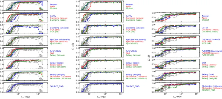
Figure 8.The product of the completeness and reliability as a function of input source flux density for each of the tested source finders for Challenges 1-3 (left to right). The grey lines show the distribution for all finders in each panel, to aid comparison for any given finder. Note that PySE (FDR) was only submitted for Challenges 1 and 2.
these but at the expense of finding many more spurious sources. This is discussed further below.
Figure 9 provides an illustration of some of the sources of incompleteness and reliability. The issue of blended sources being detected but reported as a single object by blobcat can be easily seen in this example. Here 5 adjacent pairs and 1 adjacent triplet are success-fully detected by blobcat but reported with positions, from the centroid of the flux distribution, sufficiently different from the input catalogue that they are not recognised as matches. This is likely to be the cause of the apparent reduction in completeness for blobcat at the higher flux density levels. We note that blobcat provides a flag to indicate when blobs are likely to con-sist of blended sources. These flags were not followed up for deblending in the submitted results due to the stated focus in this Challenge on point-like sources. It is clear, though, that even for point sources the blending issue needs careful attention. In a production setting, auto-mated follow-up of blended sources will be required to improve completeness. The effectively higher flux den-sity (or signal-to-noise) threshold of Apex is also visible in this Figure as the large number of sources not de-tected.
The two Selavy results shown in Figure 9 also provide insight into the possible failure modes of finders. The two algorithms shown are the “smooth” and “`a trous” methods. The smooth approach smooths the image with a spatial kernel before the source-detection process of building up the islands, which are then fitted with 2D
Gaussians. In some cases multiple components will have been blended into a single island, which is clearly only successfully fitted with one Gaussian. This leads to one form of incompleteness, probably explaining the lower overall completeness for this mode in Figure 5. The `a trous approach reconstructs the image with wavelets, rejecting random noise, and uses the reconstructed im-age to locate the islands that are subsequently fitted. This gives an island catalogue with nearby components kept distinct (which are each subsequently fit by a single Gaussian), but has the effect of identifying more spu-rious fainter islands (note the larger number of purple circles compared to the Selavy smooth case), leading to the poorer reliability seen in Figure 5. This analysis demonstrates the importance of both the detection and fitting steps for a successful finder.
4.2 Image-based accuracy measures
The method of calculating the completeness and re-liability based on source identifications depends criti-cally on the accuracy of the cross-matching. This can be problematic in the event of source confusion, where distinct sources lie close enough to appear as a single, complex blob in the image. As an alternative approach for evaluating the completeness we create images from the submitted catalogues, and compare on a pixel-by-pixel basis with the challenge images and original model images (smoothed with the same beam as the challenge images). This provides a way of assessing how well the PASA (2018)
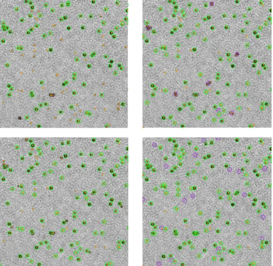
Figure 9.Examples illustrating potential sources of both incompleteness and poor reliability for four of the tested source finders for Challenge 1. Top left: Apex; Top right: blobcat; Bottom left: Selavy (smooth); Bottom right: Selavy (atrous). Orange crosses identify the location of input artificial sources. Circles are the sources identified by the various finders, with green indicating a match between a measured source and an input source, and purple indicating no match. Isolated orange crosses indicate incompleteness, and purple circles show poor reliability.
different finders replicate the distribution of sky bright-ness for the image being searched. This approach may favour over-fitting of sources, but still provides an im-portant complement to the analysis above.
The images are made using the same technique de-scribed in Section 3.2. Where available the measured size of the source components was used, but if only the deconvolved size was available the size was con-volved with the beam according to the relations in Wild (1970). This produced Gaussian blobs that were dis-tributed onto the same pixel grid as the input images to create the “implied image”. As before, the images are cropped to remove the regions where the image noise was high. We consider residual images made in two ways, by subtracting either the Challenge image or the original input model from this implied image. The following statistics were calculated from the residual:
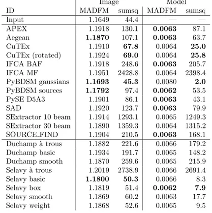
the rms; the median absolute deviation from the me-dian (MADFM, which we convert to an equivalent rms by dividing by 0.6744888; Whiting 2012); and the sum of the squares. The latter and the rms provide an in-dication of the accuracy including outliers (which will be from sources either missed or badly fit), while the MADFM gives an indication of where the bulk of the residuals lie. A finder that fits a lot of sources well, but still has a few poor fits, will tend to have a lower MADFM value but somewhat higher rms and sum of squares. The results are shown in Tables 2, 3 & 4 for Challenges 1, 2 and 3 respectively.
These statistics are related to the properties of the noise in both the Challenge and implied images. To address this in order to have some benchmark for the measured values, we perform the analysis on each of the Challenge images themselves by subtracting the
Chal-lenge image from the smoothed model. This gives the measurements that would correspond to optimal per-formance if a finder recovered the full input catalogue, given the (false) assumption that the noise is identical between the Challenge image and each implied image (i.e., some of the difference between finder metrics and the benchmark value will be attributable to noise). We note that this benchmark is only relevant for the met-rics calculated by subtracting the Challenge image from each implied image. Because the benchmark is limited by the absence of noise in the smoothed model, we treat this analysis as a relative comparison between finders rather than as an absolute metric.
blobcat does not provide shape information in the form of a major and minor axis with a position angle. Although the ratio between integrated to peak surface brightness can be used to estimate a characteristic an-gular size (geometric mean of major and minor axis), and these values were provided in the submission to the Data Challenge, they do not allow for unambiguous reconstruction of the flux density distribution and we have not included these in the present analysis so as to avoid potentially misleading results.
Different finders assume different conventions in the definition of position angle. We strongly recommend that all source finders adopt the IAU convention on position angle to avoid ambiguity. This states that po-sition angles are to be measured counter-clockwise on the sky, starting from North and increasing to the East (Trans. IAU 1974). We found that we needed to rotate Aegean’s position angles by 90◦ (an early error of con-vention in Aegean, corrected in more recent versions), and to reverse the sign of the IFCA position angles, to best match the input images. In the absence of these modifications cloverleaf patterns, with pairs of positive and negative residuals at ∼ 90◦from each other, appear at the location of each source in the residual images. CuTEx position angles were not rotated for this anal-ysis, although we found that similar cloverleaf patterns existed on significantly extended components, most no-table in Challenge 3. If we adjusted the position an-gle, though, cloverleaf residuals appeared on the more compact sources. The non-rotated catalogue performs better than the rotated version, although for complete-ness we report both versions in Tables 2, 3 and 4. The CuTEx flux densities as submitted were systematically high by a factor of two, and subsequently corrected af-ter identifying a trivial post-processing numerical error (see §4.3.2 below). The analysis here has accounted for this systematic by dividing the reported CuTEx flux densities by two.
The finders that generally appear to perform the best in this analysis are Aegean, CuTEx and PyBDSM. For PyBDSM the Gaussians mode seems to perform better than the Sources mode, across the three Challenges, al-though the performance for both is similar apart from
Challenge 3 where the Gaussians mode is more appro-priate for estimating the properties of the extended sources. The finders that seem to most poorly repro-duce the flux distribution are SExtractor and IFCA. We discuss this further below in §4.3.2.
Selavy performs reasonably well in these tests, with results generally comparable to the better performing finders. It is worth noting, though, that the different Selavy modes perform differently in each Challenge. For Challenge 1, Selavy (`a trous) performs best; for Challenge 2 it is Selavy (smooth); and for Challenge 3, Selavy (basic) and Selavy (box) both perform well. This can be understood in terms of the different source distri-butions and properties in each of the three Challenges. The high density of bright sources in Challenge 1 seems to be best addressed with the `a trous mode, the Smooth mode for the more realistic source distribution of Chal-lenge 2, and the extended sources of ChalChal-lenge 3 better characterised by the Basic and Box approaches. This leaves an open question over which mode is better suited to the properties of sources in the real sky, and this will be explored as one of the outcomes from the current analysis.
4.3 Positional and flux density accuracy
In addition to the detection properties, we also want to assess the characterisation accuracy of the different finders. This section explores their performance in terms of the measured positions and flux densities. Because not all finders report size information, we chose not to include measured sizes in the current analysis. Because the restoring beam in the Challenge images was close to circular, we also chose not to investigate position angle estimates.
4.3.1 Positions
In order to assess positional accuracy we use the re-lationships defined by Condon (1997) that establish the expected uncertainties from Gaussian fits (see also Hopkins et al. 2003). These relations give expected po-sitional errors with variance of
µ2(x0) ≈ (2σx)/(πσy) × (h2σ2/A2), (1) µ2(y0) ≈ (2σy)/(πσx) × (h2σ2/A2), (2) where σ is the image rms noise at the location of the source, h is the pixel scale and A is the amplitude of the source. The parameters σxand σy are the Gaussian σ values of the source in the x and y directions. Here, θM and θm, the full width at half maximum along the major and minor axes, can be interchanged for σxand σy, as the √8 ln 2 factor cancels. If the source size is n times larger in one dimension than the other, the posi-tional error in that dimension will be n times larger as well. In our simulations, the point sources in the PASA (2018)
images arise from a point spread function that is ap-proximately circular, and θM ≈ θm. Correspondingly, the positional rms errors in both dimensions should be µ ≈p2/π(hσ/A). For our simulated images h = 2′′, and accordingly we would expect the positional errors from a point source finder due to Gaussian noise alone to be µ ≈ 0.3′′ for S/N=5, µ ≈ 0.15′′for S/N=10, and µ ≈ 0.05′′for S/N=30.
The positional accuracies of the finders are presented in Table 5. We only show the results for Challenges 1 and 2, since the inclusion of extended sources used in Challenge 3 may result in some fraction of the mea-sured positional offsets arising from real source struc-ture rather than the intrinsic finder accuracy, making these simple statistics harder to interpret. Table 5 gives the mean and the rms in the RA and Dec offsets be-tween the input and measured source positions for each finder. All measured sources that are in common with input sources are used in calculating these statistics, for each finder. This means that finders with a higher ef-fective S/N threshold (APEX) should expect to show better rms offsets than the others, since most sources will have flux densities close to the threshold, and this is indeed the case. For most finders, with a threshold around S/N≈ 5, the best rms positional accuracy ex-pected would be around 0.3′′. For APEX, with a thresh-old around S/N≈ 10, the best rms expected should be around 0.15′′. The rms positional accuracies range from a factor of 1.3 − 2 larger than expected from Gaussian noise alone, with CuTEx, PySE and PyBDSM perform-ing the best. SAD performs as well as these finders in Challenge 2, but not quite as well in Challenge 1.
Almost all of the finders perform well in terms of absolute positional accuracy, even with the high source density of Challenge 1, with mean positional offsets typ-ically better than 10 milliarcseconds, or 0.5% of a pixel. A notable exception is SExtractor (10 beam) in Chal-lenge 1, which has a measurable systematic error in the source positions, and a significantly elevated rms in the positional accuracy. This is not present for SExtractor (30 beam) or for SExtractor in either mode for Chal-lenge 2, suggesting that it is a consequence of the high source density present in Challenge 1 and insufficient background smoothing performed in the 10 beam mode. For the two finders that we cannot assess blindly, Duchamp shows a systematic positional offset in Dec, and typically has poorer rms positional errors than most other finders. Selavy generally performs well, and over-all has good mean positions, but has poorer positional accuracy than the best of the tested finders. The Selavy mode that performs best in terms of rms positional er-ror is Selavy (weight), which is the mode that performs worst in terms of completeness. This suggests that it may be a lack of low S/N sources that is causing the es-timate of the positional error to appear better. A clear outcome of this test is that Selavy can be improved by
looking at the approach taken by CuTEx, PySE and PyBDSM in estimating source positions.
4.3.2 Flux densities
The flux density of each component was compared with the input flux density, and Figure 10 shows the ratio of measured to input flux density as a function of input flux density, for Challenge 2. Since the sources are point sources, the integrated flux density should be identical to the peak flux density, but for clarity we use reported peak flux densities from the submissions. We focus on Challenge 2 as it includes a distribution of input source flux densities most similar to the real sky. The results from Challenge 1 are similar. We do not consider Chal-lenge 3 here, again because of the bias introduced by the inclusion of extended sources with low peak flux densities and high integrated flux densities. Figure 10 indicates with solid and dashed lines the expected 1 σ and 3 σ flux density errors respectively, where σ here corresponds to the rms noise level. The dot-dashed line in each panel shows the flux ratio value corresponding to a 5 σ detection threshold. In other words, given the input flux density on the abscissa, the dot-dashed line shows the ratio that would be obtained if the measured flux density were to correspond to 5 σ. Values below (to the left) of this line are only possible if the finder re-ports measured flux densities for any source below 5 σ. This aids in comparison between the depths probed by the different finders.
The need for accurate source fitting is highlighted by the Duchamp results. Duchamp only reports the flux density contained in pixels above the detection thresh-old, and so misses a progressively larger fraction of the flux density as the sources get fainter. For this reason we do not consider Duchamp further in this discus-sion of flux density estimation. With the exception of Duchamp, all the finders implement some form of fitting to account for the total flux density of sources. They generally show similar behaviours, with reported flux densities largely consistent within the expected range of uncertainty. The CuTEx flux densities submitted were a factor of two too high, arising from a trivial numer-ical error in converting between units of Jy/beam and Jy in the post-processing of the CuTEx output. This has been subsequently corrected, and for the remainder of this analysis we consider the CuTEx flux densities after taking this correction into account.
APEX, blobcat, IFCA, PySE, and SAD all show flux density errors constrained to within 1σ for most of the range of fluxes, and IFCA in particular probes be-low the nominal 5 σ threshold while maintaining an ac-curate flux density estimate. Selavy (smooth) performs similarly well. All finders show some fraction of outliers even at high S/N (S/N> 10) with flux densities differ-ing as much as 20 − 50% from the input value. The frac-tion of measurements that lie outside the ±3 σ range is
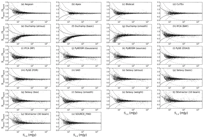
Figure 10.The ratio of the measured to the input flux density, as a function of the input flux density, for Challenge 2. The solid and dashed lines are the expected 1σ and 3σ errors from the rms noise in the image. The dot-dashed line indicates the expected flux ratio from a nominal 5 σ threshold, obtained by setting Smeas= 5 σ for all values of Sinput.
typically a few percent, ranging from 1.8% for
blob-catand SOURCE FIND, to 4.9% for PyBDSM
(Gaus-sians), and 6.5% for CuTEx after accounting for the factor of two systematic. SExtractor is notably worse, though, with more than 10% outliers in both modes. This is likely to result from assumptions about source fitting in optical images, for which SExtractor was de-signed, that are less appropriate for radio images. Selavy spans the range of the better performing finders, with 2.1% outliers for Selavy (smooth) to 4.4% for Selavy (`a trous).
Catastrophic outliers, with flux densities wrong by 20% or more at high S/N, are more of a concern, es-pecially when anticipating surveys of many millions of sources. It is possible that some (or even most) of these are related to overlapping or blended sources, where the reported flux densities are either combined from overlapping sources, or erroneously assigning flux to the wrong component. Whatever the origin, for most finders the fraction of sources brighter than 30 mJy (input flux density) with measured flux densities dis-crepant by 20% or more is 0.2 − 1%. SExtractor is
again a poor performer here, with more than 2% such catastrophic outliers. IFCA (1.1% in both modes) and PyBDSM (Gaussians) (1.9%) are notable for also hav-ing a larger fraction of such outliers. Aegean, APEX, PyBDSM (sources), PySE, and SOURCE FIND per-form the best here, all with around 0.2%. Selavy falls in the middle range on this criterion, with just below 1% catastrophic outliers in all modes.
Aegean, SExtractor, PyBDSM, and to a lesser degree PySE, show a slight tendency to more systematically over-estimate rather than under-estimate the flux den-sity as the sources became fainter. This is visible in Fig-ure 10 as a prevalence of Smeas/Sinputvalues in the +1 σ to +3 σ range and a lack between −1 σ to −3 σ. An-other way of saying it is that these finders are, on aver-age, overestimating the flux densities for these sources, compared to others that do not show this effect. Com-paring Aegean and blobcat, for example, both have almost identical completeness at these flux densities, implying that the same sources (largely) are being mea-sured, but while blobcat measures flux densities with the expected symmetrical distribution of Smeas/Sinput, PASA (2018)
Aegean shows an excess to higher ratios and a deficit at lower. This behaviour is also present for Selavy in all modes, with the possible exception of Selavy (smooth). This systematic effect is unlikely to be related to noise bias, where positive noise fluctuations allow a faint source to be more easily detected, while negative noise fluctuations can lead to sources falling below the de-tection threshold. That effect would manifest as a sys-tematic shift above (or below) the dot-dashed threshold locus, not as a deficit of sources in the −1 σ to −3 σ regime. It is also not related to any imaging biases, such as clean bias (which typically reduces measured flux densities in any case), because it is not seen in all finders. It is most likely a consequence of the approach used to perform the Gaussian fitting. At low S/N for point sources there can be more fit parameters than the data can constrain. The result is that a degeneracy between fit parameters arises, and it becomes system-atically more likely that a nearby noise peak will be mistaken for part of the same source. So the fit axes are larger and, as a result, the integrated surface brightness also goes up (see Fig. 6 of Hales et al. 2012).
Flux density estimation appears to be more complex, even for simple point sources, than might naively be expected. While the problem may be mitigated by only fitting point source parameters if the sources are known to be point-like, in practice this is rarely, if ever, known in advance. Selavy does not perform especially poorly compared to the other finders tested here, but its per-formance in all of the aspects explored above can be im-proved. None of the tested finders does well in all areas, so specific elements from different finders will need to be explored in order to identify how best to implement im-provements to Selavy and the ASKAPsoft source finder.
5 DISCUSSION
5.1 Review and comparison of finders
The purpose of this section is not to identify the “best” finder in some absolute sense, but rather to summarise the key outcomes from the above analyses, contrast-ing the performance of different finders where appropri-ate, and highlighting the areas of strength. Each of the tested finders have strengths and limitations, but none obviously perform best in all of the elements explored above. Many perform well, while still having individ-ual drawbacks or limitations. Overall, strong perform-ers include Aegean, APEX, blobcat, IFCA, PyBDSM (sources), PySE, and SOURCE FIND. A general char-acteristic in the completeness and reliability statistics seems to be that finders can maintain high reliability to low S/N only at the expense of completeness. The most accurate finders follow a similar locus in completeness and reliability below around 10 σ as illustrated in Fig-ure 8.
Aegean, blobcat, IFCA, PyBDSM (sources) and SOURCE FIND all perform similarly well in terms of completeness, reliability, positional accuracy and flux density estimation. SAD performs well with complete-ness, positional accuracy and flux density estimation, but begins to drop away in reliability below about 10 σ faster than most other finders. Aegean has a marginally higher fraction of flux density outliers than the others, and suffers from the subtle systematic at low S/N to overestimate flux densities. Aegean and SOURCE FIND perform slightly better in terms of re-liability at low S/N, but PyBDSM (sources) performs marginally better in terms of positional accuracy. IFCA in both modes performs similarly in all the elements explored. It shows the highest levels of completeness among the tested finders at low S/N but this comes at the expense of reduced reliability at these flux densi-ties. It is also accurate in its position and flux density estimation.
APEX as presented here uses a higher threshold (≈ 10 σ) for detection than the other finders. Because of this, its positional accuracy (Table 5) is about a factor of two better than nominally expected, similar in formance to Aegean and SOURCE FIND. It also per-forms similarly well in terms of flux density estimation, completeness and reliability, to the limits it probes.
PyBDSM performs very differently between the two tested modes. PyBDSM (sources) performs best over-all, with good completeness, reliability, position and flux density estimation. PyBDSM (Gaussians) is poor in terms of reliability for both Challenges 2 and 3, al-though it performed well in Challenge 1. Both modes give good positional accuracy, but PyBDSM (Gaus-sians) has a relatively large fraction of outliers and catastrophic outliers, in the flux density estimation. This is likely to be an artifact of our positional cross-matching approach selecting only the nearest submit-ted source. PyBDSM may fit a single source by many Gaussians, so if only the closest one is identified as the counterpart to the input source a lot of the flux den-sity may be artificially missed. The values shown in Tables 2 and 3 from the image-based analysis support this conclusion, especially for Challenge 3, suggesting that PyBDSM is one of the better performers in terms of reproducing the flux distribution in the image. The MADFM and sum of squares statistics, which are sen-sitive to outliers, indicate a good performance here.
PySE (D5A3) and PySE (FDR) both provide good positional and flux density estimation, but PySE (FDR) gives marginally better positions, and is more accu-rate in flux density estimation with fewer outliers and catastrophic outliers, although PySE (D5A3) probes to slightly fainter flux densities. PySE (D5A3) performs somewhat better than PySE (FDR) in terms of com-pleteness, but both are similar in terms of reliability.
CuTEx performs well in terms of positional accuracy and flux density estimation but less well in complete-ness and reliability at the low S/N end compared to most of the other finders. We note that CuTEx was not originally designed to work on radio images but on far-infrared and sub-millimetre images from space-based fa-cilities, where there is little if any filtering for large scale emission.
Those that perform particularly poorly are SExtrac-tor and Duchamp. SExtracSExtrac-tor gives a completeness and reliability that compare well to most other finders at low S/N, but with flux density estimation that is poorly suited to the characteristics of radio images. SExtractor was not designed with radio images in mind, and indeed is optimised well for the Poisson noise characteristics of optical images. It is designed to measure aperture and isophotal magnitudes in a range of ways that are ap-propriate for images at optical wavelengths, but under-standably these approaches perform more poorly in the case of radio images when compared to other tools that are designed specifically for that case. Duchamp was designed for identifying, but not fitting, sources in neu-tral hydrogen data cubes rather than continuum images, and was not expected to perform well in these tests. As expected, it performs poorly in completeness and relia-bility, as well as positional and flux density estimation, for well-understood reasons. It has been included in the current analysis for completeness.
Regarding the performance of Selavy, in the numer-ous modes tested, we have identified a number of ar-eas for improvement. Selavy (smooth) performs best in terms of flux density estimation, but is very poor in terms of completeness and reliability. Selavy (`a trous) performs better in terms of completeness, but at the expense of very poor reliability and poorer flux density estimation. The other modes of Selavy are intermediate between these extremes.
5.2 Common limitations
Inevitably, all source finders decline in completeness and reliability toward low S/N. It is therefore crucial to quantify the performance of the finder used for large surveys, in order to associate a well-defined probability of false-detection with any detected source, and to es-tablish the fraction of sources overlooked at any given S/N level. Future tests like these will ensure that the ASKAPsoft pipeline is well-calibrated in its behaviour in order to accurately quantify completeness and relia-bility.
Positional accuracy of most finders is precise and con-sistent with the expected uncertainties from Gaussian fits. However, no finders tested in this Data Challenge perform well in flux density estimation. As many as 1% of sources at high S/N may have catastrophically poor flux density estimates. These may in part be
associ-ated with blended sources since finders such as Aegean, that do well at deblending, and blobcat, that merge blended sources, show better performance here. Even Aegean and blobcat still have 0.2% and 0.4% catas-trophic outliers at high S/N, respectively (although note that blobcat flags potentially blended sources, see § 4.1). For the anticipated catalogues of tens of mil-lions of sources, this will still be a substantial number of sources. Exploring the origins of and rectifying these catastrophic errors will be an important area of refine-ment necessary for the ASKAPsoft source finder, to en-sure the high fidelity of the ASKAPsoft pipeline. 5.3 Updates since the Challenge
The Data Challenge was completed by the participating teams in early 2013. Since that time many of the source finders tested in this analysis have had continued devel-opment and improved performance. In order to retain the integrity of the Challenge and to ensure the analysis did not become open-ended, we have chosen to present the results as they are from the source finders as orig-inally submitted. In order not to provide a misleading representation of the current state of finders that have improved since that time, we give a brief summary here of some of those developments, and how they may ad-dress any of the limitations identified above.
Since the Data Challenge Aegean has continued de-velopment and the latest version can be found on GitHub1. The following enhancements and improve-ments have been made which would improve the per-formance of Aegean in this data challenge, were it to be run again:
• The Background And Noise Estimation tool (BANE, also available on GitHub) can provide more accurate background and noise images than those created by Aegean. The use of these images has been shown to increase the reliability and flux accuracy of Aegean on other real world data sets. • Aegean now produces more accurate source shape and position angle measurements for all WCS pro-jections
• A bug that cased a small systematic offset in RA/DEC has been fixed. The offset was of the order of one pixel.
• In the Data Challenge Aegean was instructed not to fit islands with more than 5 components. Islands with more than 5 components were reported with their initial parameters instead of their fit param-eters. The current version of Aegean is now able to fit the brightest 5 components and estimate the remainder. This may improve the accuracy of the
1https://github.com/PaulHancock/Aegean