VI – SIMULATION RESULTS

VI – SIMULATION RESULTS

VI.1 – Model outcomes; VI.2 – Validation; VI.3 – Description of base-case; VI.4 – Sensitivity analysis; VI.5 – Design analysis; VI.6 – Dynamic results; VI.7 – References.

VI.1 – Model outcomes

This paragraph has the task to show the performances of the model described in chap. V and its ability concerning the characterization of the system. We present here some pictures reporting interesting quantities and performance indexes.

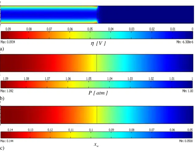
For the base-case in steady-state condition, fig. VI.1 shows the fields of a) overpotential

η

, b) pressure P, c) molar fraction of water xw, d) concentration of protonic defects cOH, e) difference of potential at local equilibrium ∆Veq (calculated as (eq. V.2.13)) and f) ratio between the module of diffusive and total flux of water in gas phase |Jw,g|/|Nw,g|.

fig. VI.1 – Pictures reporting a) overpotential; b) pressure; c) molar fraction of water; d) concentration of protonic defects; e) difference of potential at local equilibrium; f)

ratio between diffusive and total flux of water in gas phase for base-case (continue). a) ] V [ η b) ] atm [ P c) xw

fig. VI.1 – Pictures reporting a) overpotential; b) pressure; c) molar fraction of water; d) concentration of protonic defects; e) difference of potential at local equilibrium; f)

ratio between diffusive and total flux of water in gas phase for base-case (end).

It is also possible to perform boundary and domain integrations as explained in par. V.6. Fig. VI.1 demonstrates that the model of the CM is powerful and able to show several features of the system. In this way, the characterization of single phenomena and their role in the global performances of the central membrane becomes easier to understand. Thus, the model is a powerful interpretative tool that allows the analysis of the system in several ways and points of view.

VI.2 – Validation

The model is validated by using polarization curves made on 2 different samples of IDEAL-Cell. The aim of validation is to check if the model is able to reproduce the experimental behaviour of the samples.

d) OH c e) V [V] eq

∆

f)

We set the same conditions (i.e. geometry, composition of powders, porosity, working conditions, etc.) used in experiments and simulate the polarization curve by imposing several overpotential

η

CM and calculating the density of current i. In simulations we do not know 2 parameters, i.e. the exchange current i0 and the kinetic constant of water adsorption kd1. Concerning kd we set a guess value of 5·10-13mol/(m2·Pa·s); then, in sec. VI.4.2, we will perform a sensitivity analysis on it showing that it is not a key parameter that affects significantly the results. The kinetic parameter i0 is chosen by best fitting, i.e. we vary i0 in simulations in order to reproduce the experimental polarization curve.

The first sample is the same reported by Ou et al. (2009); geometry, morphology and working conditions of this sample are reported in tab. VI.1. Simulations use the same parameters2.

Class Variable Value

PCP BCY15

ACP YDC15

Materials

Gas phase water and nitrogen

T 873K Pex 1.013·105Pa xwex 5.406·10-4 Working conditions pwan 3039Pa tCM 500µm tPCE 500µm tACE 500µm rE 2mm Geometric rCM 5mm gr. dist. PCP (sys. V.4.1)

gr. dist. ACP (sys. V.4.2)

gr. dist. pore formers (sys. V.4.3)

φgfin 0.5

Morphological

ψ

PCPas 0.5

tab. VI.1 – Conditions and parameters concerning sample 1.

1 _{Note that the parameter c}

dl has not a role in polarization curves, it affects the results only in dynamic conditions.

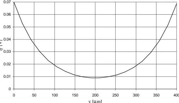
0 5 10 15 20 25 0 0.1 0.2 0.3 0.4 0.5 0.6 0.7 ηcell [V] i [A /m 2 ]

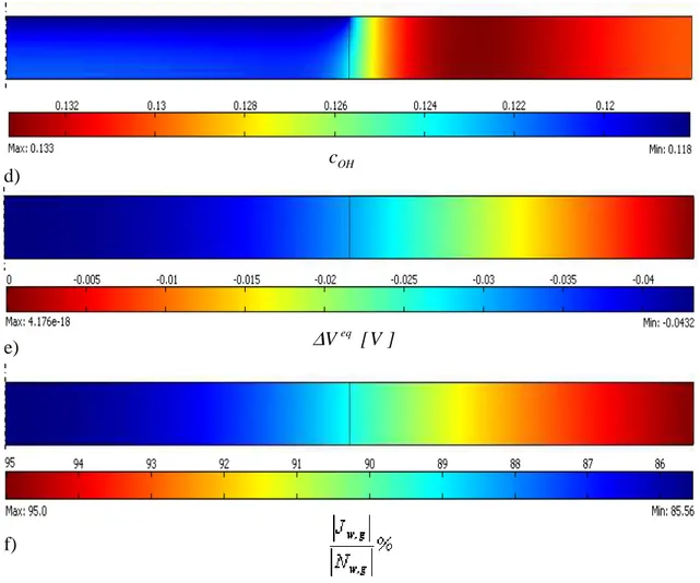
The comparison between experimental (dots) and simulated results (solid) is reported in fig. VI.2 as density of current i vs overpotential applied to the cell

η

cell calculated as:

cat ACE CM PCE an cell

η

η

η

η

η

η

= + + + + (eq. VI.2.1)

in which overpotential of anode (

η

an), cathode (

η

cat), protonic (

η

PCE) and anionic (

η

ACE) electrolyte are calculated as:

i Rp,an an = η (eq. VI.2.2) i Rp,cat cat = η (eq. VI.2.3) i t PCE PCE PCE

σ

η

= (eq. VI.2.4) i t ACE ACE ACE

σ

η

= (eq. VI.2.5)

fig. VI.2 – Comparison between experimental (dots) and simulated polarization curve for sample 1.

The conductivity of anionic electrolyte is taken equal to σACP = 1.5488S/m (tab. V.3), the conductivity of protonic electrolyte3 as σPCE = 1.562S/m. Polarization resistances of

3 _{This value is equal to the conductivity of PCP at the anodic side assuming a concentration of protonic} defects in equilibrium with partial pressure of water pwan, i.e. by using (eq. IV.3.15). Then, conductivity is calculated by using (eq. IV.4.4) with σPCPsat _{from tab. V.3.}

electrodes, made in platinum (Thorel et al., 2009), are respectively Rp,an = 3·10-4Ωm2 and Rp,cat = 4.2·10-4Ωm2 (Vladikova, 2010).

In simulations we use as parameter for water recombination reaction i0 = 8·10-9A/m, with this choice the agreement is good; in other words, i0 comes from the best fitting of the experimental polarization curve in fig. VI.2. It is important to note that the main resistances are due to the CM, ηCM/ηcell is in the order of 96% or more: this means that in sample 1 the resistances (i.e. overpotentials) due to electrodes and electrolytes are negligible if compared to the resistance of the CM, so the experimental polarization curve can be read as related to the behaviour of the central membrane alone.

The linear dependence in fig. VI.2 hints that the CM is in ohmic regime, i.e. losses of electric potential are mainly due to ohmic resistances rather than to resistances related to electrochemical reaction or gas transport (see par. V.5). It means that in this situation the key parameters are the apparent conductivities of ACP and PCP; kinetic parameters, such as kd and i0, have only a marginal role. This hints that if the description of the morphology and in particular the estimation of the correction factor σapp/σ had not been good, we would not have had the agreement shown in fig. VI.2 whatever i0 we had used. Let us make an example to explain this concept.

Imagine that the correction factor σapp/σ was smaller than the one used due to a bad estimation of it (for example, if we had used θ < 15°), in this case the simulated polarization curve would have a smaller slope, i.e. at the same overpotential ηcell the density of current i would be lesser than the value reported in fig. VI.2. Thus, to match simulated results with experimental results we would have increased the kinetic parameter i0 in order to increase the slope of the simulated polarization curve4. The asymptotic limit is related to i0 → +∞: in this situation the losses in CM are due only to ohmic resistances because the electrochemical kinetics occurs easily, so the slope of the polarization curve is only due to the apparent conductivities of ACP and PCP. If this limit slope is lesser than the slope of the experimental polarization curve there is not anything that we could do in simulations in order to obtain a good agreement with experimental results.

A second validation is made by comparing experimental polarization curve made on a different sample (Presto, 2010), called sample 2, with simulated results. The procedure that we follow is the same as described before for sample 1. Tab. VI.2 shows conditions

4

It is straightforward to understand that, fixed other parameters and conditions, the density of current i increases as the kinetic parameter i0 increases because water recombination reaction becomes easier.

and parameters concerning sample 2 and used also in simulations. We set the same kinetic parameters used for the previous validation, i.e. kd = 5·10-13mol/(m2·Pa·s) and i0 equal to 8·10-9A/m. Fig. VI.3 shows the comparison between experimental results (dots) and simulated results (solid) for sample 2: the agreement is quite good.

Class Variable Value

PCP BCY15

ACP YDC15

Materials

Gas phase water and nitrogen

T 873K Pex 1.013·105Pa xwex 2·10-4 Working conditions pwan 3039Pa tCM 700µm tPCE 577µm tACE 683µm rE 2.5mm Geometric rCM 5mm gr. dist. PCP (sys. V.4.1)

gr. dist. ACP (sys. V.4.2)

gr. dist. pore formers (sys. V.4.3)

φgfin 0.45

Morphological

ψPCPas 0.5

tab. VI.2 – Conditions and parameters concerning sample 2.

Note that also sample 2 is in ohmic regime as shown by the linear behaviour of the polarization curve in fig. VI.3. It is important to emphasize that the kinetic parameters used, and in particular the exchange current i0, are the same in the two validations: it is a significant result that the agreement is good in different cases (i.e. different samples and working conditions) with the same kinetic parameters. This fact hints that the model represents with a good accuracy the real behaviour of the system.

0 5 10 15 20 25 30 35 40 45 0.000 0.100 0.200 0.300 0.400 0.500 0.600 0.700 0.800 0.900 1.000 ηcell [V] i [A /m 2 ]

fig. VI.3 - Comparison between experimental (dots) and simulated polarization curve for sample 2.

A stronger validation is needed because, as explained above, in ohmic regime key parameters are apparent conductivities of ACP and PCP, other phenomena (i.e. water recombination kinetics, transport in gas phase, etc.) become negligible. To have a stronger validation we must compare simulations with experiments performed on samples at different regimes, for example a regime where the reaction or the transport in gas phase are determining. In other words, we could say that we have indirectly validated the submodel concerning the charge transport and the model that describes the morphology (in particular the estimation of apparent conductivity as in par. III.4).

Thus, new samples and new measurements are needed; just with these first results and with the help of the model it is possible to design cells in which the main behaviour is the one that we want to check. In this way, a stronger validation of the model (and of submodels too) will be possible.

VI.3 – Description of base-case

Since there are several unknown or uncertain parameters, a sensitivity analysis in order to understand the role and the weight of each parameter on the global performance of the CM is needed. Before starting the sensitivity analysis, an accurate description of the base-case in steady-state conditions is necessary in order to understand the effects of

0 20 40 60 80 100 120 140 0 0.1 0.2 0.3 0.4 0.5 0.6 0.7 0.8 0.9 1 ηCM [V] i [A /m 2 ]

each phenomenon (i.e. gas transport, water transport in PCP, etc.) and the global behaviour of the CM.

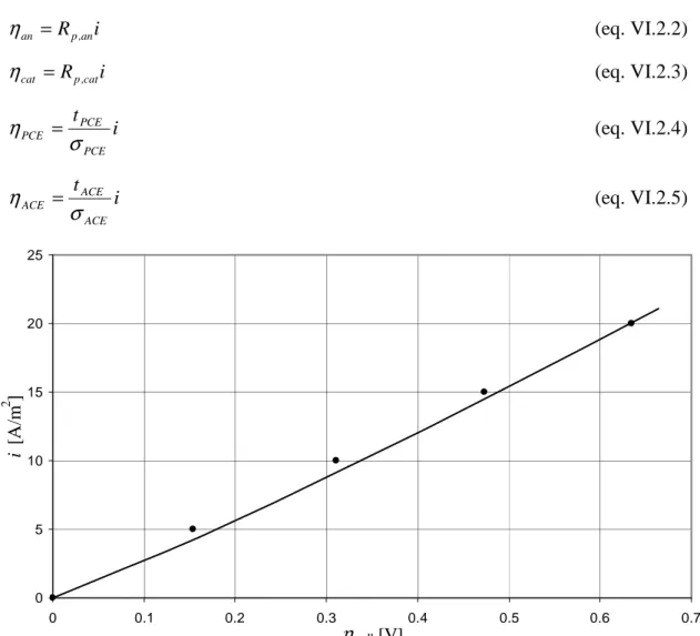
The base-case is representative of a central membrane close in its features to samples 1 and 2 used in par. VI.2 for the validation (compare tab. V.4 with tab. VI.1-2)5, i.e. base-case is representative of the actual state of the art. A confirmation to this assertion is reported in fig. VI.4 that shows the simulated polarization curve for base-case: note that the linear dependence of density of current i from overpotential ηCM hints that the CM is in ohmic regime such as samples 1 and 2.

It is interesting to note that water recombination reaction occurs close to the interfaces of CM with electrolytes: fig. IV.1a shows that the overpotential η, that is linked to the rate of water recombination is as in (eq. V.2.11), is positive only in the regions close to the electrolytes, in the remaining volume of the CM η approaches zero, i.e. reaction does not occur. This feature is evident also in fig. VI.5 that shows the overpotential η along the thickness of the CM on the axis of symmetry of the cell in the same condition (i.e. base-case in steady-state conditions for ηCM = 0.3V); note that y = 0µm means CM-anionic electrolyte interface and y = 400µm means CM-protonic electrolyte interface.

fig. VI.4 – Simulated polarization curve for base-case.

5

The major differences are represented by a smaller porosity (0.4 instead of 0.5 or 0.45) and by the radius of the cell that is 2 times bigger than in samples 1 and 2.

0 0.01 0.02 0.03 0.04 0.05 0.06 0.07 0 50 100 150 200 250 300 350 400 y [µm] η [ V ]

fig. VI.5 – Overpotential vs axial coordinate on the axis of symmetry in base-case.

It is straightforward to understand that the CM in base-case is not optimized because reaction occurs only in a small portion of the volume of the membrane, the remaining volume is useless. Remember also the considerations made in par. V.5: where η is close to zero the energy is spent in dissipations instead of in reaction. So it means that the central part of the membrane, about from y = 50µm to y = 350µm, is characterized by dissipation of energy due to ohmic resistances and it is useless. This behaviour is typical of ohmic regime: reaction occurs only in a small portion of the membrane, the remaining part contributes to increase the losses of potential for the transport of charges (i.e. it is an ohmic dissipation).

Results reported in fig. VI.1b-c concerning pressure and molar fraction of water are predictable: pressure is maximum in the center of the membrane and decreases along the radius, molar fraction of water behaves in the same way. Water produced in the reaction must be evacuated towards the outer atmosphere: the resistances to water transport produce an increase of driving forces, i.e. pressure and molar fraction of water. It is interesting to note that pressure does not increase much while molar fraction of water in the center of the CM is about 3 times bigger than in the outer atmosphere. This aspect hints that water evacuation is mainly due to separative flow (i.e. diffusion due to gradient of partial pressure of water) instead of non-separative flow (i.e. transport due to gradient of total pressure). Fig. VI.1f confirms this hypothesis: the ratio |Jw,g|/|Nw,g| is

bigger than 85%6, i.e. water is mainly evacuated by diffusion. Concerning the gas transport, Knudsen numbers are in the range Knw = 3.986-4.354 for water while for nitrogen KnB = 2.340-2.555: it means that gas transport is in transition region, so the submodel described in par. IV.2 and used in these simulations is right (as expected by the consideration made in par. IV.2 concerning the range of pressure 0.435-17.03atm in which gas transport is in transition region).

It is very important what fig. VI.1d shows because it is not expected: the concentration of protonic defects7 cOH is not uniform throughout the CM and, in particular, it is lower in the inner part of the membrane: it means that where reaction occurs (and where protons are carried) the conductivity of PCP is not the highest (remember the relationship between cOH and σPCP as in (eq. IV.4.4)). In particular, the minimum value of 0.118 represents the concentration of protonic defects in equilibrium with gaseous water at the anodic side. It is reasonable that due to the difference of concentration of protonic defects between CM and anode, they diffuse towards the anodic side: the decrease of cOH in the inner part of the CM, compared with the concentration of defects close to the outer atmosphere, is a direct consequence of this diffusive flow. Without this effect, we could expect that cOH is higher where partial pressure of water pw is higher. Note also that the maximum of cOH is reached at about x = 6.7mm: here there is the compromise between partial pressure of water and the diffusion towards the anode.

Finally, fig. VI.1e shows the difference of potential at the local equilibrium ∆Veq within the CM, in particular according to (eq. V.2.13) it follows the partial pressure of water pw. Note that in the inner part of the CM (where the reaction occurs) ∆Veq is not negligible if compared with overpotential η: it means that we should expect that when pw increases the effects of ∆Veq will become significant. In particular, when pw increases ∆Veq decreases, so η decreases at a fixed value of difference of potentials VACP – VPCP: it means that the effect of an increase of pw goes against the occurring of water recombination reaction8.

6 _{Note that |J}

w,g|/|Nw,g| is lower in the middle of the CM and higher at rCM. It is reasonable because the molar average velocity vm is higher at the axis of symmetry and decreases along the radial coordinate. Thus, the convective component of the flux of water is higher in the middle of the CM, so |Jw,g|/|Nw,g| is lower at the axis.

7

Remember that the concentration of protonic defects represents also the concentration of water adsorbed in PCP, see par. IV.3 and in particular (eq. IV.3.10).

8 _{This consideration is obvious because if the concentration of the product of the reaction (i.e. water in} gas phase) increases the rate of the reaction decreases. But the knowledge of ∆Veq

in each point of the CM is important to quantify this effect.

47.188 0 5 10 15 20 25 30 35 40 45 50

0.E+ 00 1.E-08 2.E-08 3.E-08 4.E-08 5.E-08 6.E-08 7.E-08 8.E-08 9.E-08 1.E-07

i0 [A/m]

i

[A

/m

2 ]

VI.4 – Sensitivity analysis

After the accurate description of the base-case made in the previous paragraph, it is possible to show the sensitivity analyses on unknown (i0, kd) or uncertain (σapp/σ, Dw,PCP) parameters. An analysis on the variation of external molar fraction of water xwex is performed too.

VI.4.1 – Sensitivity analysis on i0

The kinetic parameter of water recombination reaction is a key parameter: fixed other parameters and conditions, if it is high the CM is in ohmic regime (i.e. the ohmic losses are determining, ηCM is mainly spent in ohmic losses), if it is low the CM is in kinetic regime (i.e. water recombination reaction is determining, ηCM is mainly spent for the occurring of the reaction).

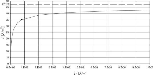
We have obtained a value of i0 = 8·10-9A/m in par. VI.2 but we have also said that it is uncertain because the estimation was made in ohmic regime where it is difficult to get accurate values concerning electrochemical reaction. In the base-case, fig. VI.6 shows the effects of a variation of i0 in a wide range on the density of current i in steady-state conditions; the estimated value of 8·10-9A/m is marked with a dot.

fig. VI.6 – Sensitivity on i0: effects on density of current in the base-case.

As expected, i decreases if i0 decreases and vice versa. But it is interesting that 2 regimes are highlighted: for small values of i0 (kinetic regime) there is a strong dependence of i on i0, at high values of i0 (ohmic regime) the dependence is mild and an asymptotic limit of i = 47.188A/m2 is reached.

The features of kinetic and ohmic regime are also shown in fig. VI.7 where overpotential η along axial coordinate y on the axis of symmetry is reported for several values of i0. At i0 = 8·10-8A/m the CM is in ohmic regime: note that the overpotential η is positive only close the CM-electrolytes interfaces, i.e. reaction occurs only in a small region, the internal part of the membrane is useless and contributes to increase losses due to ohmic resistances. At i0 = 8·10-11A/m the CM is close to kinetic regime: overpotential η is quite uniform along the thickness, so the whole membrane is used for the occurring of the reaction. Remember also that the difference ηCM – η represents all the dissipations of energy not related to electrochemical reaction (see par. V.5) and ηCM is equal to 0.3V: note that in kinetic regime these dissipations are low while in ohmic regime they are very high.

fig. VI.7 – Profiles of overpotential η along the axial coordinate at several kinetic parameters i0 for the base-case.

Fig. VI.6 demonstrates an important consideration that we have already expressed: in ohmic regime it is difficult to estimate i0 with accuracy. It is straightforward to understand that in ohmic regime small errors on i produce big errors in the estimation of

i0. For example: i = 42A/m2 corresponds to i0 = 6.9·10-8A/m while i = 42.42A/m2, i.e. an increase of 1%, to i0 = 8.3·10-8A/m, i.e. an increase of 20%. Thus, we may say that the value of i0 = 8·10-9A/m obtained in par. VI.2 in ohmic regime is only the minimum

0.00 0.05 0.10 0.15 0.20 0.25 0.30 0 50 100 150 200 250 300 350 400 y [µm] η [ V ] i0 = 8·10-11A/m i0 = 8·10-10A/m i0 = 8·10-9A/m i0 = 8·10-8A/m

34 35 36 37 38 39 40 41 42

1.E-16 1.E-15 1.E-14 1.E-13 1.E-12 1.E-11 1.E-10 1.E-09 1.E-08 1.E-07 1.E-06 1.E-05 1.E-04

kd [mol/(m2·Pa·s)]

i

[A

/m

2 ]

kinetic parameter, i0 could be much higher for the reasons explained above9. This consideration leads to think that a stronger validation of the model is needed and, in particular, the kinetic parameter i0 must be estimated in kinetic regime10.

VI.4.2 – Sensitivity analysis on kd

The assumed value of kd = 5·10-13mol/(m2·Pa·s) is a guess, specific measurements must be performed to estimate this kinetic parameter; moreover, it could be that also the kinetic law is not as in (eq. V.2.14). The sensitivity analysis, performed in the base-case at steady-state, wants to show how much a variation of kd affects the global performance of the CM, in particular the density of current i. Fig. VI.8 shows these results (the dot represents the value assumed of 5·10-13mol/(m2·Pa·s)).

fig. VI.8 – Sensitivity on kd: effects on density of current in the base-case.

Fig. VI.8. shows that if kd increases also i increases and vice versa: it is possible to explain this behaviour because if the rate of water adsorption in PCP increases also the conductivity of PCP increases, so it produces an increase of current.

There are 2 asymptotic limits and their genesis is not difficult to explain. For low values of kd the adsorption is negligible, so the concentration of protonic defects cOH is

9 _{Fig. VI.6. could be quite misleading because it seems that for i}

0 = 8·10-9A/m small errors in i do not produce big errors on i0. This is true because fig. VI.6 is related to base-case, remember that samples 1 and 2 are different and, in particular, they are closer to the asymptotic ohmic regime. For ηCM = 0.3V, in the base-case i = 35.08A/m2, i.e. the 74.5% of the limit current if i0 was infinity; at the same overpotential for sample 1 i = 9.21A/m2 while the limit current is 11.633A/m2, i.e. sample 1 is at the 79.2% of the limit. It means that sample 1 is closer to the asymptotic ohmic regime, so small errors on i produce big errors on

i0, bigger than we could expect by watching fig. VI.6 without this explanation. 10

We will see in the following that the kinetic regime is reached by decreasing the thickness tCM of the central membrane.

determined by the diffusion; in particular, there is a uniform distribution of protonic defects and cOH is equal to the concentration of protonic defects at the anode (i.e. 0.118). For high values of kd the water adsorption is very quick, so cOH follows the field of partial pressure of water pw and, in particular, cOH is equal to cOHeq in each point of the CM.

The effects of water adsorption affect also the total pressure and the molar fraction of water in gas phase. For example, for kd = 5·10-17mol/(m2·Pa·s), Pmax = 1.092atm and xw,max = 0.144; for kd = 5·10-4mol/(m2·Pa·s), Pmax = 1.006atm and xw,max = 0.0562: it is evident that if the kinetics of water adsorption is slow, water in gas phase is not adsorbed so pressure and molar fraction are higher; if the kinetics of adsorption is quick water is adsorbed in PCP from gas phase yielding a decrease on pressure and molar fraction in gas phase. These results are not obvious: if kd increases, also the density of current i increases (fig. VI.8) so in the CM more water is produced. This leads to think that the increase of water production could yield an increase of pressure and molar fraction in gas phase but it does not happen. We could say that there are two opposite effects: the increase of kd yields an increase of i that leads to an increase of P and xw, at the same time it yields an increase of adsorption of water in PCP that leads to a decrease of P and xw. The second effect wins on the first one.

Concluding, the variation of kd affects the behaviour of the CM but we may say that the effects on the global performances of the system are not so consistent: the density of current in base-case varies from i = 34.89A/m2 to i = 40.90A/m2. The kinetic constant of water adsorption is not a key parameter in ohmic regime but a specific estimation is needed in order to characterize better the behaviour of the central membrane. In particular, according with the effects of a variation of kd on gas phase as shown above, this kinetic parameter should be a key parameter in gas transport regime.

VI.4.3 – Sensitivity analysis on σapp/σ

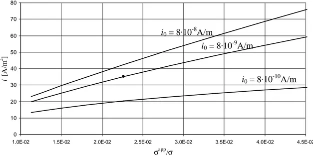
The estimation of apparent conductivities is made by using results obtained in sec. III.4.5, so the corrector factor σapp/σ is an uncertain parameter. Remember that it is used for the estimation of apparent conductivities (sec. V.4.4) and apparent diffusivity of water in PCP (sec. V.4.5). Fig. VI.9 shows the sensitivity analysis on σapp/σ in the base-case by reporting the density of current i at several exchange currents i0 (remember that also i0 is an unknown parameter). The situation representative of the base-case, i.e. with

i0 = 8·10-9A/m and σapp/σ = 2.265·10-2 as used in all other simulations, is reported with a dot.

fig. VI.9 – Sensitivity on σapp/σ: effects on density of current in the base-case.

Fixed i0 at 8·10-9A/m, fig. VI.9 shows that there is a strong dependence of the density of current i on the correction factor σapp/σ: it is a key parameter. This behaviour is predictable because the CM is in ohmic regime, so if the apparent conductivities of PCP and ACP increase also the density of current i increases quite linearly. It is interesting to note that the dependence is stronger (i.e. the slope of the curve is bigger) if i0 increases because in this case the membrane is going towards a stronger ohmic regime and vice versa (remember fig. VI.6-7).

Fig. VI.9 can also be read under the following point of view. In validation (par. VI.2) we have estimated i0 from polarization curves: if there were small errors in the estimation of σapp/σ, the errors in the estimation of i0 would be high. Note, as an example, that the same density of current i = 35.08A/m2 is obtained for i0 = 8·10-9A/m and σapp/σ = 2.265·10-2 but also for i0 = 8·10-8A/m and σapp/σ = 1.82·10-2. So, it means that in validation an error of about 20% on the estimation of the corrector factor σapp/σ could produce a different estimation of the kinetic parameter i0 of one order of magnitude.

Concluding, the correction factor σapp/σ is a key parameter and its estimation must be done with accuracy; in particular, its role is very important in ohmic regime.

0 10 20 30 40 50 60 70 80

1.0E-02 1.5E-02 2.0E-02 2.5E-02 3.0E-02 3.5E-02 4.0E-02 4.5E-02

σapp_/σ i [A /m 2 ] i0 = 8·10-9A/m i0 = 8·10-8A/m i0 = 8·10-10A/m

34.90 34.92 34.94 34.96 34.98 35.00 35.02 35.04 35.06 35.08 35.10 1 2 3 4 5 6 7 8 9 10 β i [A /m 2 ]

VI.4.4 – Sensitivity analysis on Dw,PCP

The diffusivity of water in PCP Dw,PCP is not an unknown parameter, its estimation is done as described in sec. V.4.5 according to Coors (2007). Suksamai and Metcalfe (2007) found values of Dw,PCP about 10 times higher than Coors (2007) as if self-diffusivities of protonic defects and oxygen vacancies DsOH and DsVO were 10 times higher.

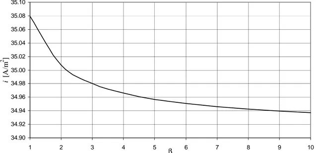
Thus, a sensitivity analysis is performed as follows: Dw,PCP is estimated according to Coors (2007) by using (eq. V.4.6-8), the result is multiplied by a factor β that varies from 1 to 10 (so, β = 1 means that we are using Coors estimation, β = 10 means that we are using Suksamai and Metcalfe estimation). Fig. VI.10 shows the results in terms of density of current i vs β for the base-case.

fig. VI.10 – Sensitivity on Dw,PCP: effects on density of current in the base-case.

Fig. VI.10 shows that the effect of the variation of Dw,PCP is negligible, the density of current i decreases only of 0.4% while Dw,PCP increases by 10 times. Note that if Dw,PCP increases the density of current i decreases: this happens because if the diffusivity of water in PCP is higher there is an higher flow of protonic defects from CM to anodic side through the protonic electrolyte. Thus the concentration of protonic defects cOH decreases (especially close to the CM-protonic electrolyte interface), so there is a reduction of conductivity of PCP that yields a lower density of current i.

The last conclusion is confirmed also by fig. VI.11 that shows the ratio Fw(PCE)/Fw(r) (i.e. the ratio between the flow of water that leaves the CM passing through the protonic electrolyte and goes towards the anode and the flow of water produced in water

0.0 0.1 0.2 0.3 0.4 0.5 0.6 0.7 0.8 0.9 1.0 1 2 3 4 5 6 7 8 9 10 β Fw (P C E ) /F w (r ) %

recombination reaction) as a function of β: if β increases (i.e. if Dw,PCP increases) the flow of water that leaves the CM by diffusion across the protonic electrolyte increases.

fig. VI.11 – Effect of an increase of diffusivity of water in PCP on the flow of water that leaves the CM in adsorbed form through the protonic electrolyte.

VI.4.5 – Sensitivity analysis on xwex

The external molar fraction of water xwex is not an uncertain parameter, it is a working condition that we have assumed in order to obtain stable and reproducible results in experiments, i.e. comparable with simulated results (see sec. V.4.7). It is interesting to investigate how performances of CM change for a variation of xwex.

Simulations are performed in base-case by varying the working condition xwex maintaining the same value of difference of potential at terminals E = 0.8163V11, i.e. the overpotential applied to the CM ηCM is not constant. This configuration is equal to work with a cell connected with an external electric device that works at a constant value of difference of potential equal to 0.8163V.

It is straightforward to understand that if xwex increases, OCV decreases, so also ηCM decreases yielding lower density of current i as reported in fig. VI.12 (the dot indicates the condition of xwex = 0.05 as in the base-case).

11

This value is equal to OCV – ηcell calculated at 600°C assuming wet hydrogen at the anode at 1atm (i.e. partial pressure of hydrogen equal to 0.97atm, the same value used in all other simulations as explained in sec. V.4.7), air at 1atm at the cathode (i.e. partial pressure of oxygen equal to 0.21atm) an wet nitrogen at 1atm in the third chamber with xwex = 0.05. In ηcell we neglect contributions of overpotentials of electrodes and electrolytes (i.e. ηcell = ηCM) with ηCM = 0.3V. Thus, E = 0.8163Vmeans ηCM = 0.3V for xwex = 0.05, i.e. the same working condition of the base-case.

0 5 10 15 20 25 30 35 40 0.001 0.01 0.1 1 xw ex i [ A /m 2 ]

fig. VI.12 – Effect of a variation of external molar fraction of water in base-case at fixed difference of potential at terminals of the cell.

It is interesting to note that the increase of density of current for small xwex is poor while the decrease of i for high values of xwex becomes significant. In particular, these effects are not only due to the variation of OCV, i.e. of ηCM, because in that case the dependence would be linear (with xwex in logarithmic scale) as demonstrated by fig. VI.13 in which overpotential applied ηCM (and used in simulations to obtain the previous figure) is reported as a function of xwex. Seeing that the dependence of density of current i from overpotential ηCM is linear as shown in fig. VI.4, by watching fig. VI.13 we could expect a linear dependence of i from the logarithm of xwex but it does not happen, it is evident in fig. VI.12.

The explanation of the behaviour in fig. VI.12 is related to the effect of the difference of potential at local equilibrium ∆Veq. If external partial pressure of water is low, a little increase of pw inside the central membrane is enough to create a significant decrease of

∆Veq according to (eq. V.2.13) that leads to a reduction of the rate of water production, so a decrease of density of current i. When pwex is high (e.g. pwex = 0.5atm) the same increase of pressure does not lead to big variation of local equilibrium condition, so the negative effects of ∆Veq on the global performance of the CM are negligible12.

12

In other words, when external partial pressure of water is low, the effects of a variation of pw from pw ex on local equilibrium are significant and vice versa.

0.00 0.05 0.10 0.15 0.20 0.25 0.30 0.35 0.40 0.45 0.50 0.001 0.01 0.1 1 xwex η C M [ V ]

fig. VI.13 – Overpotential ηCM as a function of external molar fraction of water in order to obtain a constant value of difference of potential at terminals.

Concluding, the global performance of the central membrane increases if the external molar fraction of water decreases but the increase of OCV is partly balanced by the negative effects of the local equilibrium (i.e. ∆Veq).

VI.5 – Design analysis

There are several design variables that can be modified in order to increase the performance of the CM. In particular, starting from the base-case, we will investigate the effects of a variation of morphological (i.e. final porosity, mean dimension of particles) and geometric (i.e. radius of CM, thickness of CM or protonic electrolyte) starting input parameters.

VI.5.1 – Variation of final porosity

The final porosity φgfin can be varied by changing the amount of pore formers in the mixture of particles before sintering fixed other conditions. Tab. V.1 shows the effects of a variation of porosity (i.e. a variation of volume fraction of pore formers before sintering ψf) on morphological parameters, in particular if φgfin increases the length of TPB per unit volume λvTPB decreases while the mean diameter of pores dp increases. Another important effect is on the apparent conductivities of ACP and PCP: fixed all

other conditions, if porosity increases the correction factors σapp/σ decreases as reported in sec. V.4.4

The effects of a change of porosity in the base-case are reported in fig. VI.14 as polarization curves.

fig. VI.14 – Effect of change of porosity on the performance of the CM in base-case.

The increase of porosity reduces the slope of polarization curve, i.e. at the same overpotential applied to the CM ηCM the density of current i is lower if the porosity is higher. This effect is mainly due to the decrease of apparent conductivities (σapp/σ becomes 3.093 times lower passing from porosity of 0.4 to 0.5): an increase of porosity produces a decrease of apparent conductivity of both ACP and PCP, so in ohmic regime it leads to a strong decrease of performance.

Also the length of TPB per unit volume λvTPB decreases when φgfin increases (λvTPB becomes 2.995 times lower passing from porosity of 0.4 to 0.5), the effects are the same of a decrease of the kinetic parameter i013. But in ohmic regime this effect is really negligible if compared with the effect due to the reduction of σapp/σ: comparing fig. VI.6 and fig. VI.9 it is straightforward to understand that a decrease of λvTPB (i.e. as there was a decrease of i0) by about 3 times has a lower effect than a decrease of σapp/σ of about the same magnitude.

However, an increase of porosity leads to lower performances. This happens because the evacuation of water through the gas phase is easy, if it was difficult an increase of

13 _{Note that in (eq. V.2.1-2) and (eq. V.2.4) there is always the product isλ}v

TPB, i.e. i0 is always coupled with λv

TPB and vice versa.

0 20 40 60 80 100 120 140 0 0.1 0.2 0.3 0.4 0.5 0.6 0.7 0.8 0.9 1 ηCM [V] i [A /m 2 ] φgfin = 0.4 φgfin = 0.45 φgfin = 0.5

φgfin would give higher values of density of current i at a fixed ηCM14. The demonstration that gas transport is easy and that it remains easy increasing porosity is shown in tab. VI.3, where several indexes are reported for φgfin = 0.4 and 0.5 when i = 35.08A/m2 (i.e. for ηCM = 0.3V at φgfin = 0.4 and ηCM = 0.82V at φgfin = 0.5). The reduction of Knudsen numbers, maximum pressure and flow of water evacuated by protonic electrolyte towards anode, coupled with the increase of diffusive component in water transport, show that gas transport is easy and it remains easy for φgfin = 0.4-0.5. Note that the improvements of gas transport are relatively low when porosity increases, this happens because transport in gas phase is already easy for porosity of 0.4.

porosity index 0.4 0.5 Knw 3.986-4.354 2.767-2.903 KnB 2.340-2.555 1.624-1.704 Fw(PCE)/Fw(r) 0.624% 0.298% |Jw,g|/|Nw,g| 85.56-95% 89.37-95% Pmax [atm] 1.092 1.049

tab. VI.3 – Several performance indexes concerning gas transport for porosity equal to 0.4 and 0.5.

The conclusions are that in ohmic regime porosity must be reduced in order to increase apparent conductivities of ACP and PCP. This is true until the CM does not enter in gas transport regime: if gas evacuation was the rate determining step of the process it should be reasonable to increase the porosity. At this state of the art this situation is really far.

VI.5.2 – Variation of mean dimension of particles

The mean dimension of particles is a morphological parameter that we may change. In sec. V.4.2 we showed that the actual granulometric distributions of powders are reproduced as in (sys. V.4.1-3). The simulation of the variation of dimension of particles is performed as follows: we multiply each radius rji (where j is the phase, i.e. PCP, ACP or pore formers) for the same factor γ (e.g. rPCP1 becomes equal to

14 _{We are talking about a hypothetic situation in which electrochemical kinetics and charge transport are} easy while gas transport meets high resistances. In this regime, that we have called gas transport regime in par. V.5, the performance of the CM is strictly dependent on gas transport: the rate of water production (so the density of current i) is determined by the rate of evacuation of the product of the reaction.

γ·0.054µm) with γ = 1, 1.5 or 2. So, it is equal to move towards right the granulometric distributions reported in fig. V.3. All other starting input parameters remain the same of base-case.

Polarization curves at several mean dimensions of particles are reported in fig. VI.15.

fig. VI.15 – Effect of variation of mean dimension of particles in base-case.

At the same overpotential ηCM the density of current i decreases if the mean dimension of particles (i.e. γ) increases; in other words, we may say that the slope of the polarization curve decreases as γ increases. This result is predictable because an increase of dimension of particles leads to a reduction of the length of TPB per unit volume λvTPB while apparent conductivities remain the same15. The reduction of λvTPB leads to an increase of the resistance related to the happening of the reaction, so it is clear that this leads to a reduction of performance.

Note that despite the mean dimension of particles increases by a factor 2 (and, in particular, λvTPB decreases by 3.9 times), the decrease of the density of current i is only of 15-19%. This is reasonable because the CM is in ohmic regime, so variations concerning parameters related to reaction do not change significantly the global performance of the system.

Concerning the gas phase, the increase of the mean dimension of particles leads to an increase of the mean diameter of pores, so gas transport becomes easier. Tab. VI.4 shows several indexes concerning gas transport obtained for the same density of current

15 _{As explained in sec. III.4.5, σ}app_{/σ does not depend on particle size.}

0 20 40 60 80 100 120 140 0 0.1 0.2 0.3 0.4 0.5 0.6 0.7 0.8 0.9 1 ηCM [V] i [A /m 2 ] γ = 1 γ = 1.5 γ = 2

i = 35.08A/m2 for γ = 1 (i.e. ηCM = 0.3V) or γ = 2 (i.e. ηCM = 0.367V): we could repeat the same considerations made in sec. VI.5.1 (with the analogy ↑φgfin = ↑γ).

γ index 1 2 Knw 3.986-4.354 2.112-2.209 KnB 2.340-2.555 1.239-1.296 Fw(PCE)/Fw(r) 0.624% 0.242% |Jw,g|/|Nw,g| 85.56-95% 89.35-95% Pmax [atm] 1.092 1.046

tab. VI.4 – Several performance indexes concerning gas transport for different mean dimensions of particles.

VI.5.3 – Variation of radius of the CM

At this state of the art, IDEAL-Cells have a radius of the CM rCM (and of electrolytes) that is bigger than the radius of electrodes rE (see as an example tab. VI.1-2 for existing samples of IDEAL-Cell). This feature is mainly due to technological reasons: if electrodes have a smaller radius compared with the radius of electrolytes and central membrane it is easier to separate the 3 atmospheres (i.e. anodic, cathodic and atmosphere outer of CM, see par. II.8) and to spread platinum electrodes on electrolytes (Thorel et al., 2009).

In the base-case we simulate a reduction of rCM from 10mm to 7.5mm maintaining other parameters constant, in particular the radius of electrodes, equal to 5mm, does not change. As expected, fig. VI.16 shows that maximum pressure in gas phase Pmax decreases as the radius rCM decreases: this behaviour is reasonable because gaseous water has to cover a shorter path to evacuate meeting smaller resistances.

The decrease of pressure could lead to a decrease of conductivity of PCP due to a decrease of concentration of protonic defects and it could lead to an increase of the difference of potential at local equilibrium ∆Veq. The first phenomenon leads to a decrease of density of current i, the second one produces opposite effects because if partial pressure of water (i.e. the product of the reaction) decreases the rate of water

1.070 1.075 1.080 1.085 1.090 1.095 7.5 8.0 8.5 9.0 9.5 10.0 rCM [mm] Pm a x [ at m ] 35.0 35.2 35.4 35.6 35.8 36.0 36.2 7.5 8.0 8.5 9.0 9.5 10.0 rCM [mm] i [A /m 2 ]

recombination reaction increases16. Fig. VI.17 shows that the second effect is stronger because i increases for a decrease of rCM (i.e. of pressure).

fig. VI.16 – Effect of variation of radius of CM on maximum pressure in base-case.

fig. VI.17 – Effect of variation of radius of CM on density of current in base-case.

Note that in both figures the effects are not high, in particular the increase of i due to a decrease of radius from 10mm to 7.5mm (i.e. a decrease of 25%) is equal to only 2.8%.

16

In other words, in (eq. V.2.13) if pw decreases ∆V eq

increases becoming closer to 0. So, in (eq. V.2.12), fixed the difference VACP – VPCP, an increase of ∆Veq leads to an increase of overpotential η, i.e. the rate of water production increases: this means that the density of current i increases if pw decreases. Note that

∆Veq

= -ηg,evac (see par. V.5), so all these considerations can be read as related to resistances to water evacuation.

This happens because the CM is in ohmic regime. For comparison, imagine the CM in kinetic regime (it happens for high apparent conductivities of ACP and PCP coupled with a lower value of i0) and impose the passage of a density of current i: in the whole volume η would approach ηCM so that the exchange of current is possible, i.e. water recombination reaction would occur in each point of the central membrane with the same rate. In this case, a decrease of radius rCM would lead to a decrease of reaction sites, i.e. to an increase of overpotential η to make possible the transfer of current: this means that ηCM would increase for the same density of current i, i.e. the performance of the CM, in terms of polarization resistance Rp, would decrease.

The conclusion is that in ohmic regime the radius of central membrane shall decrease to increase the performance of the system, in particular the optimal condition should correspond to rCM = rE (i.e. same radius for central membrane, electrolytes and electrodes) that leads also to saving of materials. Moreover, in order to decrease the negative effects of the increase of pressure (i.e. the decrease of ∆Veq as explained above) rCM should be reduced as much as possible. But it would mean to work with small nominal section, i.e. with small current (and small electric power) for each cell: thus, the radius of the cell is a geometric variable that must be assigned in order to reach the wished power supplied by the system.

VI.5.4 – Variation of thickness of the CM

The thickness of the CM tCM is one of the most important geometric variables. In the base-case we simulate a variation of thickness of the CM reporting polarization resistance Rp (as defined in (eq. V.6.7) with ηCM = 0.3V) as a function of the thickness. Results are shown in fig. VI.18.

Starting from base-case (i.e. tCM = 400µm), the reduction of thickness leads to a quite linear decrease of polarization resistance of the CM, i.e. it means that the performance of the system increases. For 100µm < tCM < 150µm Rp does not strongly depend on thickness and a minimum of polarization resistance is obtained for tCM = 130µm. Then, a decrease of the thickness of the membrane leads to an increase of polarization resistance that becomes very sharp for tCM < 70µm.

The explanation of the behaviour reported in fig. VI.18 is not difficult. Starting from base-case (i.e. tCM = 400µm), that is representative of a CM in ohmic regime, the decrease of thickness yields a quite linear decrease of polarization resistance because

0.000 0.005 0.010 0.015 0.020 0.025 0.030 0.035 0 100 200 300 400 500 600 tCM [µm] Rp [Ω m 2 ]

ohmic losses along the axial coordinate decrease. The reduction of thickness is as if we were removing layers from the internal region of the CM as schematized in fig. VI.19.

fig. VI.18 – Effect of variation of thickness of CM on polarization resistance in base-case.

fig. VI.19 – Schematic representation of the reduction of thickness in ohmic regime.

During the process of reduction of thickness the regime of the CM tends to become from ohmic to kinetic: reaction still occurs close to the CM-electrolytes interfaces but the reduction of thickness (in the way represented in fig. VI.19) has approached these interfaces together. It means that close to tCM = 130µm water recombination reaction occurs in the whole central volume of the CM. Fig. VI.20 agrees with this consideration: overpotential η is quite homogeneous in the central volume of the CM, compare for example fig. VI.20 (i.e. tCM = 130µm) with fig. VI.1a (i.e. tCM = 400µm).

If we reduce the thickness more, fig. VI.18 shows that polarization resistance increases. It happens because the reduction of tCM yields a reduction of the total length

of TPB used for the occurring of the reaction, so kinetic resistances increase due to the lack of reaction sites yielding an increase of Rp.

fig. VI.20 – Field of overpotential η in the base-case for tCM = 130µm.

It is important to note in fig. VI.20 that η is not equal to ηCM, so the regime is far to be completely kinetic: at tCM = 130µm the central membrane is in an optimum condition in which ohmic, kinetic and gas transport resistances are balanced together in order to yield the minimum of polarization resistance, there is not a dominant regime. To have an idea of gas transport resistances, fig. VI.21 shows the field of ηg,evac (that is equal to –∆Veq): in the central part of the CM (i.e. where η is quite homogeneous) the overpotential related to gas transport resistances ηg,evac is in the range 0.07-0.0874V, i.e. it represents the 23-29% of the overall overpotential ηCM = 0.3V applied to the membrane. Tab. VI.5 shows other performance indexes related to gas transport.

fig. VI.21 – Field of overpotential ηg,evac in the base-case for tCM = 130µm.

Knw 3.120-4.354

KnB 1.831-2.555

Fw(PCE)/Fw(r) 0.534% |Jw,g|/|Nw,g| 63.42-95%

Pmax [atm] 1.395

tab. VI.5 – Several indexes concerning gas transport in base-case for tCM = 130µm.

η [V]

Concluding, the reduction of the thickness of the CM leads to an improvement of performance until an optimum is reached at about tCM = 130µm. Note that in the neighbourhood of the optimal condition polarization resistance is quite independent on thickness: this is a good feature because little shifts of thickness near the optimal condition do not produce sharp decreases of performance.

It is also important to emphasize that a central membrane with these features (i.e. in base-case with tCM = 130µm) would be ideal to validate the model: as already explained in par. VI.2, validation should be done on a CM in which all phenomena are balanced and have the same importance.

VI.5.5 – Variation of thickness of the protonic electrolyte

The thickness of the protonic electrolyte tPCE is a geometric variable that affects the performance of the central membrane only because it is related to the transport of water in PCP through the protonic electrolyte17: fixed all other conditions, the flow of adsorbed water passing across the protonic electrolyte decreases as the thickness of this layer increases and vice versa.

In the base-case we have fixed tPCE = 50µm, fig. VI.22 shows the effects on density of current i of an increase of thickness up to 500µm18 in base-case. If the thickness of protonic electrolyte increases, the density of current i increases. This effect is due to the increase of concentration of protonic defects inside the CM: in base-case the flow of protonic defects (i.e. of adsorbed water) is from the CM towards the anode, if the thickness of the protonic electrolyte increases this flow is reduced, so the concentration of protonic defects inside the CM is higher. This consideration agrees with fig. VI.23 in which the ratio between flow of water that evacuates the CM passing through the protonic electrolyte and the flow of water produced in water recombination reaction Fw(PCE)/Fw(r) is reported as a function of tPCE for the base-case: Fw(PCE)/Fw(r) decreases when tPCE increases as expected.

It is important to emphasize that these effects do not affect significantly the performance of the central membrane, in particular the density of current i increases of 0.18% passing from tPCE = 50µm to 500µm.

17 _{In particular, t}

PCE enters in boundary conditions as reported in (sys. V.3.3). 18

We do not perform simulation with tPCE < 50µm because in this situation protonic electrolyte becomes too brittle for practical applications.

35.07 35.08 35.09 35.10 35.11 35.12 35.13 35.14 35.15 50 100 150 200 250 300 350 400 450 500 tPCE [µm] i [A /m 2 ] 0.600 0.605 0.610 0.615 0.620 0.625 50 100 150 200 250 300 350 400 450 500 tPCE [µm] F w (P C E ) /F w (r ) %

fig. VI.22 – Effect of variation thickness of protonic electrolyte on density of current in base-case.

fig. VI.23 – Effect of an increase of thickness of protonic electrolyte on the flow of water that leaves the CM in adsorbed form through the protonic electrolyte.

Concluding, an increase of the thickness of the protonic electrolyte does not affect significantly the performance of the central membrane. On the other hand, it is reasonable that the increase of the thickness of the protonic electrolyte leads to a linear increase of ohmic losses of the electrolyte (i.e. according to Ohm law) that will affect negatively the performance of the whole cell. At this state of the art, the losses related to electrolytes (and electrodes too) are only a small fraction of the global losses of the cell, i.e. ηcell ≈ ηCM as we showed in par. VI.2.

This aspect has a technological importance. The mechanical resistance of the cell is obviously proportional to its thickness; it means that at least a layer among electrolytes and central membrane must be thick enough in order to guarantee an adequate mechanical resistance. On the other hand, we have seen that to decrease losses of energy a reduction of thicknesses is needed. At this state of the art, it is reasonable to entrust the mechanical resistance to one of two electrolytes because their ohmic losses are small if compared with resistances of the CM. Thus, the electrolyte that combines the best compromise between ohmic resistance (related to the conductivity of the material) and mechanical resistance (related to the brittleness of the material) will be the thickest one19.

VI.6 – Dynamic results

All the results reported in previous paragraphs were obtained in steady-state conditions; in this paragraph, results concerning dynamic simulations of impedance, performed as explained in par. V.7, will be shown.

Fig. VI.24 shows the simulated impedance curve obtained in the base-case with external molar fraction of water xwex equal to 0.03 and an oscillating overpotential applied ηCM·sin(ωt) (with ηCM = 0.3V); impedance z is calculated as (eq. V.7.8) by using the 19th oscillation (that is stable for each frequency)20 to calculate integrals in (eq. V.7.2-3). We do not use xwex = 0.05 of the base-case because in such case there would be problems concerning initial conditions and equilibrium as explained in par. V.7. We mean that in this condition (i.e. with the same partial pressure of water at the anodic side and in the outer atmosphere surrounding the CM) a simulated and an experimental impedance curve will be definitely comparable. On the other hand, if pwex is not equal to pwan the system needs of a stabilization time to reach a stable initial condition: we can consider this time in simulations by starting the impedance test when the CM has reached the steady-state condition (i.e. by using steady-state condition as initial condition) but it is unknown in experiments, so simulated and experimental results could not be directly comparable due to different initial conditions considered.

19 _{It is straightforward to understand that it is impossible to entrust mechanical resistance to the CM} because its thickness must be small (in the order or 130µm as in sec. VI.5.4) and because it is intrinsically brittle due to the porosity.

20 _{In particular, impedance curve obtained by using density of current i(t) at the 19}th _{oscillation is the} same as we used i(t) at the 9th oscillation. It means that after (at least) 8 oscillations the response is stable for each frequency.

fig. VI.24 – Simulated impedance curve of the CM in base-case with xwex = 0.03.

The simulated impedance curve shows a first arc of impedance on the left that is related to capacitive effects in the central membrane. The maximum is reached at a frequency of 50Hz. This is a consequence of the assumed value cdl = 5·10-2C/(m2·V): if it was higher the maximum would be reached at a lower frequency and vice versa. This consideration comes from a simple analogy with a R1+(R2//C) circuit (reported for clarity in fig. VI.25a) that shows the same behaviour (fig. VI.25b, the same of fig. II.7f), at least for f > 5Hz: in this case, the pulsation of the maximum of the arc is equal to 1/(R2C) where C is the capacitance of the system. It is straightforward to understand that for the CM the overall capacitance C is proportional to the capacitance of the double layer cdl, so if cdl increases the pulsation at which the maximum is associated decreases and vice versa. At the moment, the value used for cdl is only a guess; in the future, after a stronger validation of the model, also this kinetic parameter will be estimated by comparison with experimental impedance curves.

fig. VI.25 – Analogy with an equivalent circuit: a) circuit R1+(R2//C); b) its impedance curve. 0.E+ 00 1.E-04 2.E-04 3.E-04 4.E-04 5.E-04 6.E-04 7.E-04 8.E-04 9.E-04

6.0E-03 6.5E-03 7.0E-03 7.5E-03 8.0E-03 8.5E-03

z' [Ωm2 ] -z '' [Ω m 2 ] 50Hz 5Hz R1 R2 C a) R1 R1+R2 Z’ -Z’’ R2/2 b) C R 1 2 max = ω

Note that for f → ∞ the impedance curve shows z’ ≈ 6.6·10-3Ωm2, it is representative of a big ohmic contribution (compare simulated results in fig. VI.24 with the equivalent circuit in fig. VI.25). This feature is reasonable because the CM is in ohmic regime (note that the case represented is very close to base-case). In other words, the value of z’ at f → ∞ is representative of ohmic losses in the CM and their contribution is very significant. For comparison, the difference between z’ at f = 5Hz and z’ at f → ∞ represents the contribution of resistance related to water recombination reaction, this difference is about 1.2·10-3Ωm2, so 5.5 times lower than the ohmic contribution.

For frequency lower than 5Hz a second arc of impedance is obtained (in fig. VI.24 only the first part is visible). This arc is due to resistances concerning transport in gas phase. When f is low, the reaction has got a long time to occur during an oscillation, so when the overpotential applied ηCM(t) is positive water is produced, when it is negative water is consumed. If the transport in the gas phase is not quick enough, when water is produced it accumulates in the gas phase surrounding the reaction site, so locally the partial pressure of water increases. It leads to a decrease of difference of potential at local equilibrium ∆Veq that increases the losses related to the electrochemical kinetics: the final result is an increase of resistance of the CM21, i.e. a second arc in the impedance curve is obtained.

This explanation concerning the genesis of the second arc is realistic if we consider that gas transport in CM is mainly due to diffusion since |Jw,g|/|Nw,g| approaches 1 (see for example fig. VI.1f and tab. VI.3-4), so it is reasonable that diffusive gas transport is slow if compared with rate of accumulation of water due to electrochemical reaction. Moreover, the considerations about accumulation of water into gas phase and effects of

∆Veq are supported by fig. VI.26 that shows the fields of partial pressure of water pw and difference of potential at local equilibrium ∆Veq for f = 1Hz when t = 19.5s (i.e. in the middle of the 19th oscillation when the production of water has just finished and water consumption is starting, i.e. ηCM(19.5s) = 0 and ηCM(19.5s+dt) < 0), i.e. when in each point pw and |∆Veq| are maximum in the time.

21 _{We could say that where the reaction occurs, the accumulation of water in gas phase reduces ∆V}eq , i.e. in that region the rate of water recombination reaction decreases (and it could become zero) due to a decrease of overpotential η. So, if in that region the reaction becomes difficult to occur, it means that reaction will occur in other points of the CM; but those points are not representative of optimal condition of reaction because, if they were optimal points, they would have been used before. Just make an example: fig. VI.1a shows that reaction occurs close to CM-electrolyte interfaces, this configuration is optimal, i.e. it is representative of the best that the CM can do in these conditions. If in dynamics water accumulates close to CM-electrolyte interfaces, reaction must occur in other regions, for example in more internal points. But this configuration (i.e. reaction occurring in the middle of the CM) is not optimal, i.e. it yields lower performance.

0.0E+ 00 2.0E-04 4.0E-04 6.0E-04 8.0E-04 1.0E-03 1.2E-03 1.4E-03 1.6E-03 0.006 0.008 0.01 0.012 0.014 0.016 0.018 0.02 0.022 0.024 z' [Ωm2 ] -z '' [Ω m 2 ]

fig. VI.26 – Fields of a) partial pressure of water b) difference of potential at local equilibrium for f = 1Hz at t = 19.5s in the same conditions of fig. VI.24.

An experimental impedance curve (Presto, 2010), made on sample 2 (i.e. tab. VI.2) with an oscillating input η(t) = 0.5V·sin(ωt), is reported in fig. VI.27; it is important to emphasize that fig. VI.27 is the impedance curve of the whole cell and not of the only central membrane.

fig. VI.27 – Experimental impedance curve of the whole cell for sample 2. pw [atm]

a)

∆Veq [V] b)

Despite working conditions, geometries and morphologies of sample 2 and base-case are different, simulated and experimental impedance curves show a similar shape, i.e. the presence of two arcs (in particular the second one has the highest maximum) with a big contribution due to ohmic losses. It is clear that a direct comparison between fig. VI.24 and fig. VI.27 is not possible because working conditions, geometries and morphologies are different; moreover, fig. VI.27 shows the experimental impedance curve of the whole cell (i.e. electrodes + electrolytes + CM) while fig. VI.24 shows the impedance curve of the CM alone.

Thus, we may say only that simulated impedance curve shows a similar behaviour compared with experimental impedance curve but we can not say more. In particular, we can not state that in the experimental curve the first arc is related to capacitive effects in CM and the second arc to gas transport effects in CM because in the impedance curve of the whole cell also contributions of electrodes and electrolytes are considered. It is not possible at the moment to interpret with certainty experimental impedance curves due to the overlapping of several effects. A direct comparison will become possible when the model of the whole cell will be considered and, in particular, it will be possible in simulations to distinguish each dynamic behaviour for each layer (i.e. anode, cathode, CM, protonic and anionic electrolyte). Actually, it is not possible to obtain the experimental impedance curve for each component, in particular it is not possible to perform a measurement of impedance on the CM alone.

Concluding, the model allows performing dynamic simulations and, in particular, to obtain simulated impedance curves for the central membrane. In a working condition close to base-case, the simulated impedance curve shows two arcs: the first arc is related to capacitive effects, the second one is due to resistances in gas phase. Also an experimental curve shows a similar shape but a direct comparison (or a sure interpretation) is not possible. Only with the model of the whole cell will be possible to compare experimental and simulated dynamic results, obviously if the same working procedure will be adopted (see par. V.7).

VI.7 – References

Coors W.G., “Protonic ceramic steam-permeable membranes”, Solid State Ionics, 178, pp. 481-485; 2007.

Ou T., Delloro F., Nicolella C., Bessler W.G., Thorel A.S., “Mathematical Modelling of

Mass and Charge Transport and Reaction in the Central Membrane of the IDEAL-Cell”, SOFC-XI ECS Transactions 25, pp. 1295-1304; 2009.

Suksamai W., Metcalfe I.S., “Measurement of proton and oxide ion fluxes in a working

Y-doped BaCeO3 SOFC”, Solid State Ionics, 178, pp. 627-634; 2007.

Thorel A.S., Chesnaud A., Viviani M., Barbucci A., Presto S., Piccardo P., Ilhan Z., Vladikova D., Stoynov Z., “IDEAL-Cell, a High Temperature Innovative Dual

mEmbrAne fueL-Cell”, SOFC-XI ECS Transactions, 25, pp. 753-762; 2009. Presto S., internal report, 2010.