Università degli Studi di Ferrara
DOTTORATO DI RICERCA IN
SCIENZE DELL’INGEGNERIA
CICLO XXVCOORDINATORE Prof. Stefano Trillo
Geostatistical modelling of PM
10
mass concentrations with satellite
imagery from MODIS sensor
Settore Scientifico Disciplinare ING-INF/03
Dottorando Tutore
Dott. Campalani Piero Prof. Mazzini Gianluca
_______________________________ _____________________________
(firma) (firma)
A first heartfelt thanks goes to all the people who helped me getting the research activity started, going through it and progressing until the final accomplishment. These are for sure my supervisors — Prof. Gianluca Mazz-ini, Dr. Simone Mantovani and Prof. Peter Baumann — who made it all possible; all my daily colleagues from MEEO Srl who made it all enjoyable and constructive; my research companion Thi Nhat Thanh Nguyen for the precious discussions and cooperations; Prof. Klaus Sch¨afer (IMK-IFU) and Dr. Angela Benedetti (ECMWF) for the review and assessment of this thesis; Prof. Edzer Pebesma (IFGI) and Prof. Roger Bivand (NHH) for their superb activity as community mentors inside and outside the R-Sig-Geo world; last and expected, my whole family and friends.
v · ∼
Technically speaking, my studies could not be possible without being fed with data. Further acknowledgements are due:
Pm Mapper aot products, for allowing high-resolution aerosols information inputs, which were possible thanks to the various modis software develop-ment and support teams for the production and distribution of the modis data.
Nasa software development and support teams for the production and dis-tribution of the modis data.
ii
TheAeronet teams for collecting, processing, and making available ground-based aerosol observations around the world.
The Umweltbundesamt and Arpa Emilia Romagna monitoring net-works for the provision of PM10 ground measurements.
The Ifs (Integrated Forecast System) of the Ecmwf (European Centre for Medium-Range Weather Forecasts) and Zamg (Zentralanstalt f¨ur Meteo-rologie und Geodynamik) for the meteorological maps over Austria.
1 Introduction 1
1.1 Remote sensing from satellites . . . 3
1.1.1 The physics of the problem . . . 7
1.2 Aerosols and aerosol optical thickness . . . 9
1.3 The relationship between PM and AOT. . . 13
1.4 Air quality guidelines . . . 16
2 Input Data Description 19 2.1 Aerosol optical thickness retrieval . . . 20
2.1.1 AERONET uplooking sunphotometers . . . 20
2.1.2 MODIS AOT algorithm . . . 21
2.1.3 PM MAPPER AOT . . . 25
2.2 Ground measurements of PM . . . 27
2.2.1 ARPA Emilia Romagna network. . . 28
2.2.2 Austrian network . . . 29
2.3 Auxiliary data . . . 30
2.3.1 Meteorological data . . . 31
2.3.2 Digital Elevation Model (DEM) . . . 32
2.3.3 Night lights . . . 33
3 Spatial Modelling and Online Analytics 35 3.1 Review of modelling techniques . . . 36
3.2 Kriging predictions . . . 41
3.2.1 Cokriging . . . 48 iii
iv CONTENTS
3.2.2 Kriging with regression . . . 50
3.2.3 Spatio-temporal kriging . . . 52
3.3 Web mapping and Web-based analysis of the results . . . 55
4 Models Performance and Overall Achievements 63 4.1 Validation of 1×1 km2 AOT products . . . 64
4.2 Study over Emilia Romagna . . . 73
4.3 Study over Austria . . . 80
4.3.1 Separate daily variograms . . . 82
4.3.2 Spatio-temporal interactions . . . 91
1.1 Example of MODIS granules of AOT. . . 2
1.2 Global orbit tracks of Terra satellite. . . 6
1.3 Components of solar radiation perceived by a satellite. . . 8
1.4 Hazy sky caused by tiny aerosols in the low troposphere . . . 10
1.5 Particle hazards for human health . . . 11
2.1 Linear regression between surface reflectances in the visible and SWIR channels. . . 24
2.2 The two-step cascade architecture of PM MAPPER.. . . 26
2.3 PM MAPPER AOT product samples.. . . 27
2.4 Layout of ARPA ER air quality ground stations (black points). 28 2.5 Mother domain of the WRF simulations for meteorological fields 31 2.6 Examples of original 3 arcsec DEM from SRTM: a cutout over the river Po in Emilia Romagna (Italy).. . . 32
2.7 Cutout of nighttime lights average over Emilia Romagna . . . 33
3.1 Photo of the planetary boundary layer over Berlin . . . 40
3.2 Kriging interpolation principles . . . 42
3.3 Variogram concepts . . . 46
3.4 1D example schema of kriging with regression . . . 51
3.5 Web-based analysis of geostatistical data . . . 57
4.1 Satellite-sunphotometer coupling . . . 65
4.2 ER-diagram of the validation database . . . 66
4.3 AOT Validation 3D surfaces templates . . . 67 v
vi LIST OF FIGURES
4.4 AOT Validation surfaces: number of matches. . . 68
4.5 AOT Validation surfaces: linear correlation . . . 68
4.6 AOT Validation surfaces: mean error . . . 69
4.7 AOT Validation surfaces: root mean square error . . . 70
4.8 Validation scatterplots and QQ-plots . . . 71
4.9 MEA-PM Web interface for air quality data visualization.. . . 74
4.10 General workflow of the air quality models on Emilia Romagna 75 4.11 Statistical models of cokriging . . . 76
4.12 Cokriging cross-validation outcomes over Emilia Romagna. . . 78
4.13 Variogram examples from the study on Emilia Romagna . . . 79
4.14 Orography and night lights over Austria . . . 81
4.15 General workflow of the study over Austria for pure spatial modelling . . . 84
4.16 Percentage of available AOT pixels over Austria (2009) . . . . 85
4.17 The role of AOT in the PM10 regression over Austria (2008) . 86 4.18 Example of a daily PM10 gap-filling over Austria for different interpolation methods. . . 90
4.19 AOT-METEO daily scatterplots . . . 93
4.20 Pooled PM10 variograms . . . 95
4.21 A PM10 3D experimental variogram . . . 96
4.22 X-validation RMSE for ST-KED model in 2010. . . 97
4.23 Pooled PM10 temporal variograms . . . 98
2.1 The seven MODIS channels that are used in the AOT inversion algorithms. . . 23
2.2 Exceedances rate of PM10 in Austria from 2006 to 2008. . . . 30 4.1 AOT 1×1 km2 validation scores . . . . 72 4.2 Percentage of AOT pixels over Austria (2008 to 2010). . . 85
4.3 Cross-validation statistics for the prediction of PM10over Aus-tria . . . 88
4.4 Cross-validation seasonality for the prediction of PM10 over Austria . . . 88
4.5 Cross-validation statistics for the spatio-temporal prediction of PM10 over Austria . . . 97 4.6 Examples of WCPS responses for model-based 3D series of
images. . . 100
Chapter 1
Introduction
The purpose of the research activity carried out in these last three years puts its roots when the Earth Observing Systems (EOS) Terra satellite (originally called EOS-AM-1 because of its morning crossing time through the equator,
Levy et al. 2009) was successfully launched in 19991 by NASA, and began
collecting data on February 24th, 2000. The scientific data retrieved by the instruments onboard this satellite is made available to the public via Web sites and FTP archives then used in several disciplines, including oceanogra-phy, biology, and atmospheric modelling.
Several remote sensors were put onboard the Terra satellite and among these, due to its wide spectral range and good spatial resolution, the Moderate-resolution Imaging Spectroradiometer (MODIS) got very popular for research applications in different fields. Amid the long list of MODIS products (see
http://modis.gsfc.nasa.gov/data/dataprod/index.php) a strong scien-tific interest originated from the MOD04 Aerosol Product (somehow surprisingly2), and a huge amount of linked publications were written more
1Its companion – EOS Aqua – will follow in 2002.
2“The use of the MODIS aerosol products has far exceeded nearly everyone’s
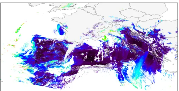
Fig. 1.1 – Example of composite of MODIS-derived AOT observations (granules) on
January 29th, 2008.
and more often, as demonstrated by Yoram Janusz Kaufman — Project Sci-entist for the Terra mission, outstanding sciSci-entist and Senior Fellow in the NASA Goddard Earth-Sun Exploration Division — in a search on the ISI citation Web site (climate.gsfc.nasa.gov).
Regarding the aerosol validated (Remer et al.,2005) products of the MODIS sensor (see Fig. 1.1 for an example), they opened a new horizon in the field of atmospheric modelling: the opportunity to deal with daily observations of the atmosphere in the form of bidimensional maps, together with the quick development of more and more powerful FOSS GIS systems and software packages for spatial data management and analysis (e.g. Baumann et al.
1998;Bock et al. 2008;Caldeweyher 2011;R Development Core Team 2011),
pushed an enthusiastic reaction of the scientific world, seeing in the remote monitoring a practical way to guard several aspects of our Earth, including climate change, radiative budget and, of course, air pollution.
This last task, which is the focus of this thesis, is however very challenging, up to the point that still after more than a decade of research publications, it is unclear when, where and whether the spaceborne aerosol maps are offering a
1.1 Remote sensing from satellites 3
strong and reliable advantage. This key point has been the drawing power of my studies, which aimed at putting more light on this unanswered question, by evaluating different geostatistical techniques on several datasets which were made available thanks to many private and public research centres (see p.i), with different combinations of sources and scales.
This introductory chapter will prepare a ground of knowledge for those who are still unfamiliar with the concepts of remote sensing, particulate matter and aerosol optical thickness. I will be explaining, in a general understand-able manner, the main problematics that arise when modelling Air Quality (AQ) concentrations at the ground level by means of spaceborne maps. A final section will describe the current guidelines with regards to the air qual-ity risk assessment and management, with a focus on the current status on the use of models for support to air quality policy in Europe.
1.1
Remote sensing from satellites
Monitoring the Earth with satellites gave rise to an increasing hope in un-derstanding what actually is behind harmful factors like climate warming, rising sea level, deforestation, desertification, ozone depletion, and so on. Satellites would help us assess current state, forecast the future impacts and take proper actions to preserve our planet.
This hope prompted the launch of a plenty of Earth-observing sensors in either the low (LEO), medium (MEO) and geosynchronous (GEO) orbits, totaling up to approximately 900 satellites orbiting above us, as currently tracked NASA (NASA, 2008). Dozens of them are currently in orbit for air quality purposes including the monitoring of sulfur dioxide (SO2), carbon
monoxide (CO), nitrogen dioxide (NO2) and ozone (O3).
temporal resolutions for aerosols detection, specifically. OMI from Aura Polar Sun-synchronous (PS) satellite (NASA) or SCIAMACHY from Envisat PS satellite (ESA), GOME-2 from METOP PS satellite and MISR from Terra itself are some examples. The unique combination of characteristics offered by MODIS determined its success in the scientific community:
Terra and Aqua platforms, both hosting a MODIS sensor, follow re-spectively a descending and ascending polar orbit from a vantage about 700 km above the surface. Although this implies a repeat cycle3 of 16
days, the MODIS sensor, with its wide view (±55◦) and consequent large swath4 (around 2330 km), is able to scan almost the whole planet
on a daily basis. To better appreciate this, Fig. 1.2 shows the orbit track of Terra. MISR sensor, onboard Terra itself, is also able to re-trieve aerosol information with comparable (if not better) quality (Liu et al., 2007b,a) but its temporal resolution up to 9 days inhibits its usage for comprehensive monitoring over an area, and it may rather be used in conjunction with MODIS, which offers more frequent over-passes.
The spatial resolution of MODIS observations is from 250 to 1000 m at nadir, depending on the spectral channel, allowing for final aerosol retrievals on 10×10 km2 boxes (the next chapter will clarify the
con-straints that cause this loss). Though not optimal for small scale anal-ysis, this resolution is still pretty high with respect to other available aerosol products: SCIAMACHY nadir-view products reach a 30×30 km2 horizontal resolution; GOME-2 80×40 km2 and OMI 13×25 km2, for instance (The World Data Center For Remote Sensing Of The Atmo-sphere,2002). Moreover, while e.g. OMI aerosol retrievals must assume aerosol layer height, MODIS is not sensitive to it and with its smaller pixel size is less affected by subpixel clouds (Satheesh et al.,2009).
3The time a satellite spends to cross the same spot on the Earth.
1.1 Remote sensing from satellites 5
The MODIS scanner has an excellent spectral width and resolution, with 36 channels covering from visible to infrared wavelengths. The aerosol retrieval algorithm makes use of 7 frequency channels and yields thorough estimates of the amounts of aerosols release into the atmo-sphere (the algorithm of the MOD04 aerosol product will be described in more detail later on).
As a final crucial factor, MODIS data are made available to the public for free download.
Although the combination of these features revealed to be highly fascinating for scientific studies, still MODIS data might not be enough for a comprehen-sible daily air monitoring: as for most spaceborne observations of aerosols, especially for passive sensors, the ability to see through clouds is prevented by the scanner wavelengths, while the horizontal resolution is still not optimal.
This last issue is what really concerns the use of the polar-orbiting MODIS retrievals for air monitoring: the regulations, as will be examined in Sec.1.4, call for specific temporal averages and frequency of occurrence of concen-tration levels for criteria pollutants. Exceedances estimations would re-quire hourly observations throughout the day, which cannot be derived from MODIS imagery. Geostationary satellites like GOES (Paciorek et al., 2008) or MeteoSat (Popp et al.,2007), provide aerosol products with high temporal resolution and this would allow both the visualization of aerosol fronts move-ment and the evaluation timing of exceedances. Their view is however fixed and still they don’t have the accuracy of aerosol estimation which MODIS has: by 2015, NOAA proposes to launch the GOES-R series of satellites, which will allow retrievals of precise aerosol products every 5—30 min (Hoff
and Christopher,2009) using MODIS-like channels. This might lead to new
1.1 Remote sensing from satellites 7
1.1.1
The physics of the problem
The AOT products which are available from sensors onboard satellites like MODIS and others are not a direct measurement, but they are obtained from a retrieval based on a physical model. Direct measurements are proportional to the reflected solar radiation that is perceived by the sensor for a certain spectral band; the contribution of aerosols to this incoming reflectance is only partial, as we will see in more detail in this section.
Earth observations are made at wavelengths from 260 nm in the ultraviolet (UV) through radar wavelengths (0.1—10 cm): the ability to see through clouds and probe down to surface exists only at radar wavelengths, thus clouds heavily condition satellite observations for air quality. The strong absorption of energy of the ozone layer (which is about 20—30 km above the surface) inhibits to see UV absorbing gases below it, in the lower troposphere. Bright surfaces like desert or snow can also mislead the sensor: the scattered radiance is too high on those areas and hence the satellite cannot discern the contribution of scattering along the atmosphere from the contribution of the surface.
To better figure out the different parts of electromagnetic radiation which contribute to the received satellite measurement, Fig. 1.3 will now be ex-plained. The incoming flux of solar radiation is scattered (and absorbed as well) by the gases and aerosol particles in the atmosphere; these rays can either be scattered somewhere on different directions, or either be directed (directly or by means of multi-scattering deviations) in the field of view of the satellite (cases 2 and 3 in the figure). The surface then reflects the in-coming radiation (components 1 and 3) back to the atmosphere which in turn will be filtered by other gases and suspended particles along the path before reaching the Top Of the Atmosphere (TOA). Other contributions of scattered light are received by the satellite sensor, i.e. the beams coming from neighbouring areas/pixels (component 4 in Fig. 1.3), and the upwelling
In-Solar
radiation
Atmosphere Target area Neighboring area Total radiance at the sensor Sensor aboard satelliteFig. 1.3 – Components of solar radiation perceived by a satellite.
fraRed (IR) radiance from the surface (not highlighted in the picture) which represents the largest source of background radiation for IR channels. These last wavelengths are however very important in cloud screening because the temperature of high, thin clouds (cirrus) are much colder than the underlying surface, clouds, and aerosols below.
In general, the radiation reflected from the surface (component 1 in the picture) is the main term of comparison with the radiation directly scattered by the particle and gases in the atmosphere, and that is indeed used by Earth-viewing satellites to extract aerosol features. The radiative transfer equation is generally written separately for the visible (dominated by the solar input and scattered light) and the IR atmosphere, where absorption and surface contribute the most. For further details refer to Thomas and Stamnes (2002).
The acquisition of aerosol features depends on physical models to account for the particle characteristics and the underlying surface reflectivity, as well.
1.2 Aerosols and aerosol optical thickness 9
Indeed, Husar (2011) points out the inherent limitations of deriving aerosol properties from the measured scattering of solar radiation, so that there is an intrinsic not negligible level of uncertainty in these data. Satellite observa-tions should not be used as unique drivers for deriving air quality information; they rather should be used in combination with models and vertical profiles coming from active profilers (lidars) to really obtain improved estimations of pollutant concentrations. The ultimate system for air quality modelling would be a collection of integrated measurement systems using geostationary passive imagers (for hourly resolution) combined with lidar rangers (vertical profiling) and integrated with ground based pollutant concentrations (Hidy et al.,2009). Sec1.3 will go through these issues in more detail.
1.2
Aerosols and aerosol optical thickness
In this section you will be introduced to the physics of the aerosol particles, their role in Earth balance and the different features that can be used to describe their nature and presence in the atmosphere. Being of absolute primary importance for both the studies carried out in this thesis and in the literature, a special remark will be given to the Aerosol Optical Thickness (AOT).
Technically, aerosols are tiny solid and liquid particles and are present through-out the atmosphere. The primary particles are introduced directly into the atmosphere, while the secondary particles are formed by chemical reactions, like gas-to-particle conversion for instance which can happen by either nu-cleation, condensation or reaction in liquid droplets (Breslow, 2002).
Key aerosol groups include sulfates, organic carbon, black carbon, nitrates, mineral dust, and sea salt (Tie et al.,2005). In practice, aerosols often bunch up together to form complex mixtures, and are mainly responsible for hazy skies (see Fig.1.4).
Fig. 1.4 – Hazy sky caused by tiny aerosols in the low troposphere (Greenland).
Aerosols can either occur naturally due to wildfires, volcanic eruptions, dust storms, suspended salts from sea spray, and plant respiration; or either they are produced by humans, from cars emissions, factories, biomass burning, and agricultural dust. Regulatory agencies use to call them Particulate Matter (PM), identifying the measured dry-mass aerosols concentrations at ground level, and usually adopted as a hint of soot, smoke and ash. Although about 90% of the aerosols in the atmosphere have natural origins, it is actually the remaining anthropogenic 10% that dominates the urban and industrial areas
(NASA Earth Observatory,2010).
Aerosols are so important because they represent an area of uncertainty within Earth’s climate system. They are like a ‘wild card’, Kaufman once explained. “They are hard to predict because they act like double agents in the system.” His point was that aerosols can cause warming — by absorbing more light than they reflect (e.g. black carbon) — or cooling — by scattering sunlight back to space (as sulfates or nitrates do) — of the Earth’s surface, depending upon their size, type, and location (http: //earthobservatory.nasa.gov/). Aerosols can enhance cloud formations or they can suppress them by interfering with the process of convection. They
1.2 Aerosols and aerosol optical thickness 11
Fig. 1.5 – Particle hazards for human health: below a diameter of 10µm of size they are
inhaled, while finer particles below 2.5µm can reach the alveoli.
can intensify precipitation, or they can suppress it. What makes it highly challenging to model is its high spatial and temporal variation, as well as its capacity to be transported for even thousand of kilometers, despite deposi-tion and cloud formadeposi-tion along the path (Slanina,1997).
Aerosols have caught large attention especially for their impact on human-health: when inhaled into the lungs, particles can be a health hazard to humans, and long exposures have been linked to asthma, poor lung devel-opment in children, cancer, and in general they cause an increase in cardiac and respiratory morbidity5 and mortality (Nel, 2005). Fig. 1.5 depicts the
different levels of inhalation of aerosol particles through the mouth based upon their size. Head and tracheobronchial deposition increase with increas-ing particle size, whereas alveolar depositions decrease for particles larger than 4 microns (Lippmann and Albert,1969).
A convenient way to estimate the presence of aerosols in the atmosphere
is the Aerosol Optical Thickness (AOT), sometimes called Aerosol Optical Depth (AOD), or simply τ . It is a unitless measure and it is defined as the integral of the atmospheric extinction coefficient from surface to space. In other words it is the degree to which aerosols prevent the transmission of light by absorption or scattering. According to the Beer–Lambert–Bouguer Law, being I0 the radiation emitted by the Sun, and I the radiation received
by the passive sensor, the total atmospheric optical thickness τ is defined as follows:
I/I0 = e−mτ (1.1)
where m is the relative airmass6. The atmospheric optical thickness can be
divided into several components: Rayleigh scattering, aerosols, and gaseous absorption. A more technical insight on the AOT inversion from measured reflectance will be treated in the next chapter, whereas for further details on atmospheric extinction and optical depths see Biggar et al. (1990).
AOT has proved to correlate with ground pollution concentrations, namely PM10and PM2.5: a consistent body of literature shows that air quality can be
assessed from this columnar satellite product (Wang and Christopher 2003;
Engel-Cox et al. 2004; Gupta et al. 2006 for example), however there are
several aspects that needs to be accounted to: AOT is indeed not equivalent to PM, and this will be better explained in the next section.
6In astronomy, air mass (or airmass) is the optical path length through Earth’s
atmo-sphere for light from a celestial source, i.e. the Sun in our case. It is usually intended as relative air mass, so that it is normalized to the air mass at the zenith (at sea level).
1.3 The relationship between PM and AOT 13
1.3
The relationship between PM and AOT
A monitoring of PM10 by remote-sensing observations would be perfectly
possible if we could build some unique relationship between AOT measure-ments and the particle mass concentrations, which however depends on many factors such as the size, chemical composition and shape of the particles. Nei-ther is this relationship clear and straightforward, nor it is fixed: it actually strongly relies on the geographical location under study, and on the meteo-rological conditions (Pelletier et al., 2007). As an example, previous studies showed promising correlations of 1-month time-series of AOT and PM2.5 for
many stations in the Eastern and Midwest USA, whereas other stations, particularly in the Western USA, did not show almost any correlation at all
(Koelemeijer et al., 2006). Again, a comparison of AOT and PM
measure-ments over the Fresno Supersite in California (Watson et al., 2012), showed clearly different empirical AOT-PM2.5 relationships by season: because AOT
was actually lowest in winter, this might have suggested that surface PM2.5
concentrations were also lowest in winter, which was however not the case!
In addition to these difficulties, both the observations have intrinsic measure-ment errors and, more important, the spatial and temporal samplings highly differ: on one side we have temporal averages of PM dry mass concentrations over a single location, on the other side we have semi-instantaneous colum-nar averages of aerosol particles over several square kilometers of area (Yahi
et al., 2011): although “human-breathing-zone” monitoring is what mostly
concerns us, most pollutants reside vertically above the surface stations.
To understand which factors can influence the relationship between AOT and surface PM, we can derive an analytical expression of it. Assuming a homogeneous atmospheric layer with spherical aerosols of density ρ, then the dry mass of sampled PM at the surface can be written as7:
PM = 4 3πρ
r3n(r) dr (1.2)
where n(r) represents the distribution of aerosol sizes in the column. Equa-tion 1.2 simply defines the sum of the weights of each single aerosol particle in the atmospheric volume (Koelemeijer et al., 2006).
It should be pointed out that aerosol particles are subject to hygroscopic growth due to humidity in the atmosphere, thus increasing the scattering power of the particles while keeping the PM dry weight fixed. The AOT at height H can then be expressed as (Hansen and Travis, 1974):
AOT = π H
0
∞
0
r2Qambext (r)namb(r) dr dz (1.3)
which, under dry conditions (so that we can include the PM definition), and solving the integral over the height, turns into:
AOT ≈ πH · f (RH) ∞ 0 r2Qdryext(r)n(r) dr (1.4) ≈ 3 · PM · H · f (RH) 4ρ · r3n(r) dr ∞ 0 r2Qdryext(r)n(r) dr · r 2n(r) dr r2n(r) dr (1.5) ≈ 3 4ρPM · H · f (RH) ⟨Qdryext⟩ reff (1.6)
where f (RH) is then the function that defines the ratio of the extinction efficiencies respectively under ambient relative humidity conditions Qamb
ext (r)
and under dry conditions Qdryext(r); ⟨Qdryext⟩ is the averaged size-distribution integrated extinction efficiency under dry conditions; and reff is the so-called
1.3 The relationship between PM and AOT 15
and defined as r3n(r) dr / r2n(r) dr.
Eq. 1.6 clearly shows how the AOT should better represent the surface dry particulate in case the scattering efficiencies changes due to humidity (f (RH)) and the height of the atmospheric layer (H), are taken into account. This can be understood by the dilution effects of the vertical mixing of the aerosols and the fact that satellites measure aerosols under humid conditions, which is not the case of the ground measuring stations of PM which derive dry-mass densities.
A further element that controls the concentration of particles in the air is temperature. On one side it can enhance the photochemical reactions in the atmosphere and hence the production of PM particles; on the other hand strong temperature inversions can keep the mixing layer at low elevations hence keeping the aerosols at surface level, inhibiting vertical mixing (Gupta and Christopher,2009b).
In conclusion, there are premises for “gap-filling” the surface-based networks, especially during well-mixed conditions with stable pressure systems where usually atmospheric aerosols correlate well with the surface. Nonetheless, the opportunity of using satellite observations to fill in surface measurements is still weakened with an understanding of the limitations of space-based measurements in adequately characterizing lower-troposphere conditions. In spite of this, it is still true that satellite observations, especially on long-term records (Van Donkelaar et al., 2009), clearly provide valuable knowl-edge of concentration distributions and can assist the air quality community (e.g. NASA-NOAA partnership).
1.4
Air quality guidelines
The World Health Organization (WHO, http://www.who.int/) is the ref-erence organization for several health-related guidelines which are offered principally to policy-makers of any developed/developing country through-out the world. Amongst these, air quality guidelines are provided: national standards can then vary, according to own local circumstances and local health risk management, linked mainly to technological, economical, politi-cal and social factors.
Guidelines for air quality are given separately for particulate matter, ozone, nitrogen dioxide and sulfur dioxide. There is still an acknowledged intrin-sic limitation in giving distinct guidelines for these pollutants, due to the complexity of air pollution mixture: nitrogen dioxide (NO2) for example is
known to be associated to UltraFine (UF) particles (i.e. PM0.1) and to be a
precursor of ozone and other toxic pollutants.
Based on the currently (Global Update 2005) available scientific evidence (Dockery et al.,1993;Pope III et al.,2002;Jerrett et al.,2005), the following guidelines for PM are suggested:
PM2.5: 10 µg/m3 annual mean
25 µg/m3 24-hour mean
PM10: 20 µg/m3 annual mean
50 µg/m3 24-hour mean
Although the majority of epidemiological studies refer to PM10, simply
be-cause PM10 routine monitoring stations are far more widespread, there are
some cases in which the distribution between the coarse (particle size be-tween 2.5 and 10 µm) and fine (particles smaller than 2.5 µm) is not equally distributed. Whereas the former are mainly produced by mechanical pro-cesses like construction activities or road dust, the latter mainly comes from
1.4 Air quality guidelines 17
combustion: hence, PM2.5 guidelines are also provided for areas where the
fine mode dominates, which are simply derived from typical fine/coarse ratios found in urban areas (0.5—0.8).
Though the annual average constraints tend to take the precedence for be-ing more restrictive, it is however over true that short-term peaks of PM concentrations can lead to equivalently dangerous effects on human health, as reported by several studies (Katsouyanni et al., 2001; Samet et al., 2000;
Ezzati et al., 2004). For this need, as well as for fining exceedances, 24-hour mean thresholds also suggested along with the annual ones.
In areas with high levels of pollution, other interim targets are proposed to encourage a gradual achievement of the final reported guidelines. Even though critical concentrations of pollutants in the air can clearly have seri-ous health consequences on the population, it should be stressed that still research has not identified thresholds below which some harmful effect does not occur, so that there is no full protection that can be ensured in any case. This is especially true for airborne particulate matter (World Health Organization, 2006).
In Europe, Air Quality Directives (AQD) are still unclear regarding the use of models for the support of AQ policies (European Commission, 2012): they simply state that “the results of modelling and/or indicative measurement shall be taken into account for the assessment of air quality with respect to the limit values”, but their role is not further explained.
The FAIRMODE group (European Environment Agency (EEA) and
Euro-pean Commission Joint Research Centre (JRC), 2008) — a forum of AQ
experts which is trying to harmonize the modelling techniques and to give inputs to the European legislation — has identified the major applications of models within the AQD, namely exceedances assessment, forecasting, source allocation and control measures assessment. This forum is trying to push changes in the current directives in order to clarify the roles of models in
the AQ policies and increase the importance of modelling estimates, up to their mandatory use. Models do not only serve as tool for assessing and han-dling the risk on certain areas, but as well can have impact on the number and optimal design of future monitoring stations, and should be used for regulatory purposes, once they have shown to fulfill some required quality objective. Still these recommendations are waiting for official responses from the European Parliament.
This section concludes the first introductory chapter. Next chapter will have a closer look at the datasets which were used in the models: feature descrip-tion, measurement instrumentation and algorithmics.
Chapter 2
Input Data Description
Different models for PM10spatial filling have been tested during this research
activity, over two areas of interest — Emilia Romagna and Austria — and with different input datasets. This section is going to describe the whole set of data sources which have been used for both modelling and validation analysis.
The chapter will start with the description of the different AOT observations that were available and used, with a focus on the MODIS inversion algorithm to let the reader understand which kind of uncertainties and approximations can arise on this product, and for different levels of spatial resolutions; sec-ondly the description will move to the ground measurements of particulate matter in Emilia Romagna and Austria, and finally to the auxiliary variables that were included in the models for further explanatory purposes.
2.1
Aerosol optical thickness retrieval
The widely used way of describing the columnar loading of aerosols in the atmosphere is by evaluating its optical thickness. Sec. 1.2 initialized the reader to the concept of AOT: in this section instead a description of two different ways of observing AOT will be proposed, namely uplooking from the ground (the ground truth) and downlooking from satellites, along with pros and cons of both measurements.
2.1.1
AERONET uplooking sunphotometers
Generally, instruments measuring the optical depth of a particular gas or substance from the ground are extremely useful mostly as they act as refer-ence for the remote-sensed observations: a means of validation of the satellite products.
The optical thickness of the aerosols is usually measured on the ground by photometers pointing to the Sun: the atmospheric effect (see component 3 in Fig. 1.3), hence the reduction of the solar flux by scattering and absorption in the atmosphere, can be removed with the so-called Langley extrapolation method: in absence of clouds and with a constant aerosols layer (at high alti-tudes) one can assume a linear relationship between the received direct-Sun radiance and the airmass, that can be inferred by repeated measurements. Extrapolating at a null airmass, the extraterrestrial Sun radiance can be measured. This can be easily observed by taking the logarithm of Eq.2.1:
ln I = ln I0− mτ (2.1)
2.1 Aerosol optical thickness retrieval 21
depth of the atmospheric can be determined.
Several networks of uplooking sunphotometry are available globally nowa-days, AErosol RObotic NETwork (AERONET) being the largest. This network, established by NASA and PHOTONS, was set up initially ∼20 years ago and now counts almost 600 sunphotometers equally spread over the Earth. Aerosol (not only optical) properties are acquired then freely distributed via either Web download tool or FTP transfer.
Measurements are taken at eight different wavelengths, namely from 340 to 1020 nm, on a preprogrammed temporal sequence starting at an air mass of 7 in the morning and ending at an air mass of 7 in the evening. Each observation is meant as a triplet of measurements over 30 seconds of time, in order to screen out clouds which usually show a much higher variance in time in their optical depth. Thanks to the wide spectrum of measurements, the contribute of the aerosols particles can be isolated by removing the attenua-tion of the smaller particles (Rayleigh scattering) and the absorpattenua-tion of ozone and other gaseous pollutants (NASA,1993). The zero air mass radiation for the calibration is inferred to an accuracy of approximately 0.2 to 0.5% thus resulting in an uncertainty of optical depths of 0.002 to 0.005. AOT products are then distributed at three quality levels: Level 1.0 (unscreened) and Level 1.5 (cloud-screened) data in near real-time; Level 2.0 quality-assured data after a longer delay for manual inspection and final calibration.
2.1.2
MODIS AOT algorithm
This section will describe the principles behind the AOT algorithms for the MODIS sensor. Specifically, Collection 005 is considered, being it the one including spectral inputs of the AOT information used in this study.
de-tails) provides a long series of products, from raw radiances to more sophis-ticated products related to atmosphere, land, ocean and crysosphere.
The aerosol products, called either MOD04 (Terra), MYD04 (Aqua) or M?D04 (both), rely on the calibrated georeferenced perceived reflectances, called Level 1B, L1B or M?D02 products. Possible errors can be associated to these raw measurements upon radiometric noise, digitization, and possible calibra-tion nonlinearities, as discussed in Ignatov et al. (2005). Further ‘Level 2’ datasets are then used in the algorithm, like the cloud mask (MYD35) and the atmospheric profile (MYD07), as will be described in the following para-graphs.
As a first distinction, due to the different radiative properties, two indepen-dent algorithms are applied over land pixels and over ocean pixels1. Both
of them are based on a ‘look-up table’ (LUT) approach, which stores pre-computed radiative transfer calculations for a finite set of aerosol and surface parameters: spectral reflectance from the LUT is compared with the mea-sured spectral reflectance to find the optimal (least-squares) fit. The models in the table take into account all the factors that influence the radiative transfer, including observation geometries, the surface type, the elevation of land and Sun. Although the input reflectances reach a resolution of 250 m, the final output maps of AOT are then distributed at an horizontal resolution of 10 km at Nadir, in order to reduce the noise in the inversion.
The first step in deriving the aerosol optical thickness is to collect spectral reflectances over different bands (for the complete set of bands used in the aerosol retrieval, see Tab. 2.1) so as to be able to screen out pixels over cloud and critical surfaces like ocean and heavy dust glints, snow and ice, which cause a high uncertainty in the AOT retrieval. These reflectances are corrected for water vapor, ozone, and carbon dioxide before the algorithm proceeds.
1The algorithm over land is selected when at least one pixel in a 10×10 box is not
2.1 Aerosol optical thickness retrieval 23
Table 2.1 – The seven MODIS channels that are used in the AOT inversion algorithms.
Band # Bandwidth (µm) Weighted Central Wavelength (µm) Resolution (m) 1 0.620—0.670 0.646 250 2 0.841—0.876 0.855 250 3 0.459—0.479 0.466 500 4 0.545—0.565 0.553 500 5 1.230—1.250 1.243 500 6 1.628—1.652 1.632 500 7 2.105—2.155 2.119 500
Only the dark pixels are considered good for the algorithm, and if there are enough pixels in the current box, then the algorithm continues with a further screening of the brightest and darkest pixels left: this is a sort of precautionary measure in order to remove remaining pixels which might have been possibly contaminated by cloud shadows, residual cloud contamination and odd surfaces at either the bright or dark end.
Once the uncertain pixels are filtered out, the retrieval estimates (over land) the contribute of the surface in the reflectance (Tanr´e et al., 1997): this is then used as in input in the LUT along with the total reflectance, to retrieve the AOT. A weighting parameter is also computed in order to balance the fine and coarse components of the aerosol model. As output of the LUT, the optical depth is finally retrieved at 0.55µm, which is often used as reference in global climate modelling.
Actually, the algorithm over land retrieves the AOT at two different chan-nels (#1 and #3) which have an established relationship with the surface reflectance (at 2.13 µm), and which is instead missing at the target wave-length of 0.55 µm and which partly define the models in the LUT. Fig. 2.1
shows the empirical linear relationships used in the MODIS algorithm (fur-ther variables of the regression are considered to refine the relationship,Levy et al. 2009).
Fig. 2.1 – Linear regression between surface reflectances in the visible (0.47 and 0.66µm
channels) and the 2.12µm SWIR channel. Image courtesy of L.A. Remer et al.
AOT is therefore interpolated by using the ˚Angstr¨om exponent α, which drives the relationship between spectral AOT and the wavelength:
α = − logτλ1
τλ2
log λ1λ2 (2.2)
These were the general principles behind the AOT inversion; for details on the algorithms over both land and ocean, refer toRemer et al. (2005).
The expected uncertainty for the optical thickness τ was found to be: ∆τ = ±0.03 ± 0.05τ over ocean
∆τ = ±0.05 ± 0.15τ over land
which generally holds independently of the output wavelength. There are only some particular conditions under which the expected accuracy of the retrieval might not be met, e.g. whit non-spherical dust over ocean or over coastal areas.
2.1 Aerosol optical thickness retrieval 25
During aerosol retrieval on a particular 10 km box, the algorithm may en-counter either non-fatal or fatal errors: quality flags are associated to each single AOT pixel, mainly to constrain out less confident data in the quality-assured Optical Depth Land And Ocean product (NASA, 1999). Inversion algorithms for MODIS are organized in Collections, the current be-ing collection 005. Collections are meant as products that are generated by similar, but not necessarily the same, versions of the algorithms. A history of changes that were applied from the initial pre-launch AOT algorithms can be found in Remer et al. (2006). The forthcoming collection 6 will include (though a first version was included already in C005) the Deep Blue algo-rithm (Hsu et al., 2004, 2006) which will increase the capabilities to extract data over bright surfaces (e.g. deserts), will improve the cloud screening, the aerosol physical models and the calibration.
2.1.3
PM MAPPER AOT
PM MAPPER is a software system for air quality monitoring applications from global- to local-scale. It consists of a two-steps cascade process, capable of handling the multispectral data input acquired by the MODIS sensors. The input and output details of the processing are shown in Fig. 2.2: the first part is a tuned version of MODIS data from IMAPP software (HUANG
et al., 2004), so as to achieve AOT products with higher spatial resolution
and higher availability (Nguyen et al.,2010a;Nguyen,2012); the second part aims at the deduction of air quality maps from the original aerosol data.
A first version of the inversion algorithm retrieved AOT data at 3×3 km2 of spatial resolution, to allow for local scale/urban areas monitoring. Validation of these product has been carried out with success byNguyen et al.(2010b), with overall good comparison with MODIS standard products and a higher capacity in retrieving AOT information over land areas, especially coastlines
Fig. 2.2 – The two-step cascade architecture of PM MAPPER.
where original MODIS products lack. Further proceedings in the algorithm could lead the retrieval up to a resolution of 1×1 km2, with increased
ca-pabilities of retrieval over bright and dark surfaces: this validated product
(Campalani et al., 2011a) was actually used in the PM10 models described
in the next chapters.
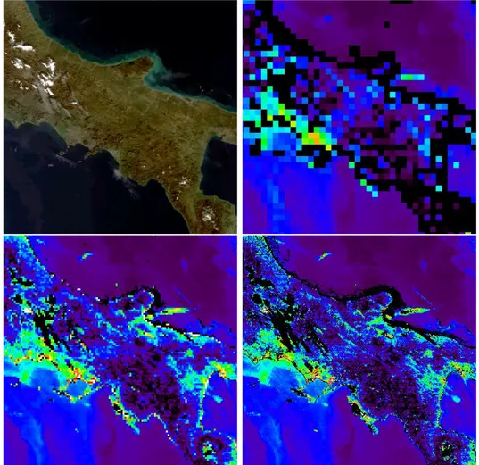
The algorithm flow is analogous to the one described in the previous sec-tion, hence essentially tries to isolate the radiative contribute of aerosols by means of several auxiliary information from surface, geometry and spectral reflectances, screening out clouds and overly bright (and overly dark) pixels. The details of the algorithm are described inMEEO Srl (2009). To perceive the kind of detail that can be expressed with a 1 × 1 km2 product, a sample
2.2 Ground measurements of PM 27
Fig. 2.3 – PM MAPPER AOT product samples at different resolution levels: 10 × 10 km2
(upper-right), 3 × 3 km2 (lower-left) and 1 × 1 km2 (lower-right) over Southern Italy.
2.2
Ground measurements of PM
Two networks of air quality ground stations were used: the first one is the net-work managed by ARPA (www.arpa.emr.it), the Regional Environmental Agency in Emilia Romagna (Italy); the second one is the Austrian Air Qual-ity network managed by the Umweltbundesamt (www.umweltbundesamt.at), the state environmental protection agency in Austria.
Fig. 2.4 – Layout of ARPA ER air quality ground stations (black points).
2.2.1
ARPA Emilia Romagna network
ARPA Emilia-Romagna (ARPA ER) is the regional agency for prevention and environment in Emilia Romagna (Italy). It is operative since 1996 and has institutional duties for:
- monitoring environmental components;
- controlling and overseeing the territory and the anthropic activities;
- supporting the evaluation of the environmental impact of plans and projects;
- realizing and managing the regional informative system of the environ-ment.
2.2 Ground measurements of PM 29
ARPA ER is delivering daily charts of PM10and PM2.5 over the whole region
by means of about 60 ground stations (May 2010). The charts contain the 24-hours mean of the measured particulate of one day, almost continuously during the period of activity of each station. Their location is visualized in Fig. 2.4: clearly there is a relatively high clustering in the pattern of the stations, inevitably because of the higher interest in measuring high polluted industrial/urban traffic areas. Exhaustive metadata on single stations can be found inCampalani and Pasetti (2010a).
For further details and technical reports, seeARPA Emilia Romagna(1995).
2.2.2
Austrian network
The measurements of PM10 for the models over Austria were taken from
the Austrian Air Quality, which currently comprises ∼160 . The data was kindly provided by the regional Austrian administrations and extracted from IDV (Immissions Daten Verbund) which is a database containing all mea-surements from the operational Austrian Air Quality network.
The Umweltbundesamt is the expert authority of the federal government for environmental protection and thus responsible for writing the State-of-the-Environment Reports, involving different areas of interest, like soil and water waste, biological diversity protection, forest use, industrial plants, etc. And of course, air. The last available report (01-2007 to 12-2009) states that the PM10emissions have increased from 2006 to 2008 by 0.5 percent from 35,400
tons to 35,600 tons; the PM2.5 emissions have instead decreased by 2 percent
from 21,500 tons to 21,100 tons. Prominent source sectors of PM10and PM2.5
emissions are industry (27% and 17%), lower consumption (29% and 44%), transportation (23% and 25%) and farmers transport community (15% and 6%).
Table 2.2 – Exceedances rate of PM10in Austria from 2006 to 2008.
Year # Exceedances rate Measuring Points
2006 64% 111
2007 20% 127
2008 12% 134
With regards to PM10 specifically, in 2006 the limit values (Sec. 1.4) were
passed to up to two thirds of all sites, with more stress over urban areas, inner-alpine valleys and basins. The decrease in exposure from 2006 to 2007 and 2008 (see Tab. 2.2) was primarily related to the less frequent occur-rence of meteorological conditions which were favorable for the air pollution: e.g. the mild winter months in 2007 and 2008 have shown less temperature inversions overall.
The Umweltbundesamt does not publish reports with technical descriptions of the monitoring methods used. For further details see Umweltbundesamt
(1999).
2.3
Auxiliary data
As underlined in Ch. 1, the aerosols atmospheric information observed by satellites is generally not enough for a direct translation to ground concen-trations. Recalling Eq. 1.6, it is clear how the relationship linking the AOT and the dry particulate is involving further meteorological and topographical information which should be embedded in the model of PM. The auxiliary variables that were included in our models are described in the next subsec-tions, namely the meteorological variables in Sec.2.3.1, the Digital Elevation Model (DEM) in Sec. 2.3.2 and the yearly averages of Night Lights (NL) in Sec. 2.3.3.
2.3 Auxiliary data 31
Fig. 2.5 – Mother domain of the WRF simulations for meteorological fields (Lambert-conformal grid, dx = dy = 27 km).
2.3.1
Meteorological data
Simulated meteorological fields of wind, temperature, pressure, relative hu-midity and planetary boundary layer height were provided on a 3-dimensional grid by ZAMG (Zentralanstalt f¨ur Meteorologie und Geodynamik), the na-tional agency of meteorological and geophysical services in Austria.
The model simulations are based on the world leading 16 km global forecasts provided by the IFS (Integrated Forecast System) of the ECMWF (European Centre for Medium-Range Weather Forecasts). This data is further processed by the Weather Research and Forecasting (WRF) Model, which uses thies fields as initial and boundary conditions, to provide forecasts of meteorology on an hourly basis. The temporal resolution of the ECMWF forecasts is 3 hours. The data is extracted on 16 pressure levels (between 10—1000 hPa) with a spatial resolution of 0.5◦ in each horizontal direction. These fields are used as initial and boundary conditions by WRF, which conducts forecasts of meteorology on an hourly basis and on 43 model levels. To obtain the
Fig. 2.6 – Examples of original 3 arcsec DEM from SRTM: a cutout over the river Po in Emilia Romagna (Italy).
data set the modelling system is setup to provide forecasts on a resolution of 27 km over the whole European domain (see Fig. 2.5).
For air quality mapping purposes, the surface-level forecasts (1000 hPa) were interpolated to at 1×1 km of spatial resolution with a cubic spline interpo-lator to meet the resolution of the PM MAPPER products. The 2D grids at surface were extracted to vertically co-locate the meteorological datasets with the PM measurements, so that they could be representative of the me-teorological conditions perceived by the ground monitoring stations.
2.3.2
Digital Elevation Model (DEM)
Elevation data was taken from the NASA Shuttle Radar Topographic Mission (SRTM) whose DEM covers over 80% of the globe. The data is distributed free of charge by U.S. Geological Survey (USGS) governmental company, available for download over a mosaiced 5 × 5 degree tiling scheme, in both ArcInfo ASCII and GeoTIFF formats (The CGAR Consortium for Spatial Information,1999).
2.3 Auxiliary data 33
Fig. 2.7 – Cutout of NOAA 30 arcsec nighttime lights average over Emilia Romagna
(9◦E − 43.5◦N to 13◦E − 45.5◦N).
The SRTM data is available as 3 arcsec (∼90 m resolution) DEMs, with a reported vertical error of less than 16 m, but it was aggregated to the resolution of 1 × 1 km2 as input for the models, being it the target resolution
of the predictions. Fig.2.6 shows a small styled cutout over Northern Italy.
2.3.3
Night lights
Yearly averages of remote-sensed night lights are available free of charge thanks to the Earth Observation Group (EOG) of NOAA Federal Agency of the U.S., by means of GeoTIFF archives.
The files are cloud-free composites made using the available archived “smooth” (quality assessed) resolution data of the Operational Linescan System (OLS) instruments onboard the several Defense Meteorological Satellite Program (DMSP) satellites which are orbiting continuously (often two satellites at the same time) from 1992. Each DMSP satellite has a 101 minute, sun-synchronous near-polar orbit at an altitude of 830 km above the surface of the Earth; the final products are 30 arcsec grids, spanning the whole globe within -65 and 75 degrees of latitude. A number of constraints are used to select the highest quality data for entry into the composites, for details refer
Chapter 3
Spatial Modelling and Online
Analytics
This chapter is dedicated to an analytical description of the geostatistical estimation and visualization tools that have been used for the assessment of PM10 concentrations over the two areas of interest we focused on: Emilia
Romagna and Austria.
Sec. 3.1 will offer an overview of the most widely used model techniques adopted in literature, explaining our decision to choose geostatistical interpo-lation and, in particular, kriging. Sec. 3.2 will describe the statistical model behind a kriging interpolation, from a simple univariate case up to more complex situations involving multiple variables as well as spatio-temporal in-teractions. Finally, Sec.3.3 will show the solutions and design choices which were made for the access of the final predictions in a Web-based scenario.
3.1
Review of modelling techniques
Before describing the mathematical and statistical basis of kriging, an overview on the different modelling solutions and research trends is proposed, along with an explanation on why kriging was chosen as estimator.
Kriging — or better said the kriging suite of geostatistical techniques — is a choice amongst the family of stochastic (least squares) interpolators; although, as we will see, it is an optimal estimator and is widely used in research for air quality assessment, it must be carefully considered before its adoption as it is not the best (nor unique) technique, in an absolute sense.
Zooming out, the geostatistical interpolation only represents a single cate-gory among the wider range of models that can be chosen for air pollution assessment. In Jerrett et al. (2004), different classes of exposure models are identified1, from simple mechanical interpolator and proximity models, to
land use regressions, to more advanced dispersion models, up to hybrid mod-els (e.g. personal monitoring + other modmod-els). Geostatistical interpolation is then an other solution, which offers advantages and disadvantages: context-specific decisions must be made to correctly optimize the available resources, research time, software, hardware and data.
The best way to measure individual exposure to air pollutants would be to use personal air monitors: the majority of the people passes around 90% of the time indoors, where usually are different concentration levels than in outdoors environments (e.g. Mukala et al. 2000; Liu et al. 1997). However, the use of this method can be prohibitive for large-scale analysis. Proximity models, i.e. risk assessment proportional to the proximity to pollution sources (e.g.Langholz et al. 2002;Maheswaran and Elliott 2003), are the most basic modelling solution but it can still be considered for a first sensitivity analysis, as a driver for further more sophisticated and costly solutions.
3.1 Review of modelling techniques 37
Land use regression models (e.g. Lebret et al. 2000; Brauer et al. 2003), which predict air pollution based on surrounding land use and traffic charac-teristics with least square regression, is able to produce statistically reliable results and also has a fair transferability2, but is mainly applied for
intrau-rban analysis and do not really account for distances of the locations and measurements.
Dispersion models (e.g. Walker et al. 1999; Potoglou and Kanaroglou 2005) can offer a more realistic fit of the theory structure by including topography, traffic observations, meteorology and pollution: the stationary and mobile emissions sources are then used as starting point to model the dispersion of pollutants. The most widely used is the Gaussian model, which assumes a (pretty unrealistic) Gaussian dispersion of the pollutants. These models require a strong cross-validation process with monitoring data, being prone to errors; they also require high-level GIS and programming expertise, and expensive hardware.
Even more complex models cascade a meteorological module to a chemi-cal one: at every time step the atmospheric conditions are modeled by the meteorological component and sent as input to the chemical dispersion mod-eler. These models are not widely used actually, having an extremely high implementation and data cost: computational requirements are huge, and high-level programming, meteorology and climatology expertise is preferred. Different types of these so-called Integrated Meteorological-Emission (IME) models exist: from the most accessible diagnostic models (e.g. ATMOS1 by
Davis et al. 1984); to the dynamical models (e.g. MM5 by Grell et al. 1994), which can simulate a much wider set of exposure scenarios; up to the most complex Four-Dimensional Data Assimilation (FDDA) models which reduce the propagation of errors (e.g. CALPUFF byScire et al. 2000).
Jerrett et al. in 2004 correctly pointed out the promising improvement in
air quality modelling upon integration of remote sensing satellite systems
data with ground monitoring network data. And actually there has been a clear trend in the last years of air quality research in the use of aerosol op-tical properties. With the increasing role of satellite observations — mainly from MODIS (Terra and Aqua) and MISR (Terra) sensors for these applica-tions — remote sensing data started to be included in the models to detect/ track particulate matter plumes from major events (e.g. dust storms, vol-canic emissions, and fires) and to fill the temporal and spatial gaps found with ground-level monitor data, the latter representing the specific context of this thesis.
After a first successful correlation study between PM10 and AOT over a
sin-gle station in Italy (r = 0.82) byChu et al. in2003, several studies aimed at developing linear regression models for estimating PM concentrations from AOT, either as a direct affine transformation or with multivariate (general-ized) linear models.
Wang and Christopher (2003) discovered very good correlations between
AOT and PM2.5 in Alabama using MODIS data (r of 0.7 with the 1-hour
averages, and even 0.98 for 24-hour averages); Kacenelenbogen et al. (2006) found good correlation too using near-polar orbiting ADEOS-2 AOT product with fine particles (PM2.5) in France.
Engel-Cox et al. in 2004 analysed the MODIS-AOT/PM ratio over the US,
finding variable correlations in the East/Mid-West areas and in the West side; the author hypothesizes this could be caused by wider variety of aerosol types (nitrate/sulfates ratios), increased presence of black carbon (soot), and higher surface reflectivities in the western US, making the AOT retrieval more difficult and more prone to uncertainty.
Gupta et al. — in 2006, 2007 and 2008 for example — developed linear
regression models over several different locations, generally finding a good association between PM ground observations and AOT, with a general weaker correlation in Winter and with a strong effect of meteorological conditions due
3.1 Review of modelling techniques 39
to relative humidity and mixing layer height3 in primis; in particular,
the author identifies ideal conditions for a stronger PM-AOT match with a 40—50% of relative humidity and a mixing layer of 100 to 200 m (in a study over global cities). Other studies confirmed the usefulness of humidity and planetary boundary layer height4, like Paciorek et al. (2008) with GOES-12
AOT products over the US or likeTsai et al. (2011) with MODIS data over Taiwan (the latter underlining how the haze layer height5 was actually better for the normalization of the AOT columnar loading, due to the abundance of aerosols aloft above boundary layer). Fig. 3.1 shows the visible difference in atmospheric conditions below and above the boundary layer.
Hutchison made several study on how to correlate MODIS AOT to the
ground-measured PM in Texas (2003, 2004, 2005 and 2008), on both the evaluation of air quality and the detection of aerosol transport; the author describes one of the first cases of joint use of AOT and aerosols vertical profiles from CALIPSO (Winker et al., 2006) lidar measurements to assess the air pollution: knowing the vertical structure of aerosol loadings actu-ally is a key information to infer the aerosol concentrations on the ground level. Van Donkelaar et al. has included (model-based) aerosol profiles along with aerosol size and relative humidity to proxy MODIS AOT for air quality assessment over Moscow (2011).
Liu et al. (2007b) built up regression models with MISR AOT data, but
us-ing separate AOT model components (fractional AOT) to predict the ground particulate (as well as sulfates and nitrates), and finding overall better re-gression fit than with total-column AOT.
3The mixing layer height determines the volume in which turbulence is active and into
which fine particles, which are emitted near the surface, are dispersed. The mixing layer shows (approximately) constant potential temperature (temperature failing at a rate of
approximately 10◦C/km).
4Layer that divides the lower turbulent atmosphere to the free nonturbulent
(geostrophic) atmosphere: it can be used as surrogate of the mixing layer.
5A layer of haze in the atmosphere, usually bounded at the top by a temperature
inversion and frequently extending downward to the ground: it is the sum of boundary and scale height, the latter being the height of a uniform extinction layer above the boundary layer, namely where the aerosol extinction coefficient decreases to 1/e.
Fig. 3.1 – The planetary boundary layer keeping the aerosol on the low (mixing) atmo-sphere over Berlin: above the layer the air is cleaner, thus the city lights are (almost) not scattered towards the viewer. Photo courtesy of Ralf Steikert.
Some studies went beyond linear regression models, by using more sophisti-cated methods like Bayesian hierarchical space-time models (Garcia et al.,
2006), recently-developed Partial-Least-Square (PLS) regression techniques (Porter et al., 2012), hierarchical dynamical coregionalisation models (Fass`o
et al., 2009), or neural networks (Gupta and Christopher, 2009a). A more
recent study in 2009 by Liu et al. applied geostationary GOES aerosol/ smoke AOD products in conjunction with land use and meteorological fields to feed a two-stage generalized additive model in Massachusetts, concluding how AOT was actually contributing actively to the prediction power of the model (even though the meteorological seemed to play a major role).
Geostationary products were used as well in recent studies by Emili et al.
(2010;2011) who investigated the predictive power of SEVIRI AOT for PM10
over the Alpine region, which showed higher correlations coefficients than MODIS for the year 2008 (0.7 against 0.6) and higher data availability (but with coarser spatial resolution); the planetary boundary layer height was also
3.2 Kriging predictions 41
found to be of key importance, whereas the role of relative humidity did not strongly influence the regression; the author finally points out the problem of accuracy in the satellite observations for complex terrains, up to the point that inverse distance interpolation could yield more accurate maps of PM10.
In conclusion, these last decade of research on air quality modelling, es-pecially by jointly exploiting the ground measurements with satellite data, produced a myriad of different results (refer to Jerrett et al. 2004 and Hoff
and Christopher 2009 for an exhaustive review), and still — as pointed out
inKumar (2010) — there are important spatio-temporal mismatches in the
datasets that are not addressed and compromise the modeled maps. Shared results can be extrapolated overall: spaceborne AOT can be potentially used to help assessing the air quality risk, though usually needs either explana-tory meteorological variables or vertical profiles to better translate the optical properties to ground-level PM concentrations.
Kriging techniques for PM assessment have also been explored recently (see
Denby et al. 2008; Kloog et al. 2011; de Kassteele and Velders 2006; Pearce et al. 2009, for instance), but the results are context-specific and the perfor-mances of kriging geostatistics still need to be further analysed, especially for daily mapping with high-resolution remote sensing, and over different topography profiles. They offer higher capabilities of prediction for spatial phenomena with respect to the simple regression models, and still do not re-quire such expensive hardware resources as more complex dispersion models would.
3.2
Kriging predictions
Kriging interpolation represents a good trade-off between the theory match with reality, data inputs, hardware resources and expert personnel required. It creates a statistical model on the available pollution and (possibly)
ex-planatory variables with knowledge of their geographic location and their (cross-)correlations, then predicts the filled map (see Fig.3.2), assigning sta-tistical uncertainty to each estimated location.
Fig. 3.2 – Kriging interpolates input measurements (black points) modeled as a stochastic variable Z ∼ N onto a regular grid (white points) which are then usually visualized as pixels of a map; the resolution of the pixels might be different from their support. Picture courtesy of Tomislav Hengl.
Giving the error structure of the estimates is actually a feature which dis-tinguishes kriging (and model-based geostatistics in general) from both em-pirical interpolators and more complex dispersion models; it can be useful to either compute confidence intervals for threshold exceedances, or to visually see which areas of the output prediction are less certain (intuitively areas far away from the available inputs).
With respect to simple mechanical interpolator — like inverse distance weight-ing, nearest neighbour, splines, Thiessen polygons — kriging estimates the value at the new unobserved location in an objective way, following prob-ability theory. Validation or cross-validation procedures can also be easily computed against the input concentrations measurements.
Kriging can be run in ordinary machines with relative low computational resources6 and with free software, as with R packages like geoR (Ribeiro Jr
and Diggle,2001) and gstat (Pebesma,2004).
6Few minutes of computation on Intel(R) Core(TM)2 Duo CPU [email protected] with
3.2 Kriging predictions 43
Kriging interpolation works well in case the statistical assumptions are met, and in case there is a sufficient number of unclustered target observations, so that the spatial pattern (covariances) can be described with statistical significance and with sufficient level of detail relatively to the spatial gradients of variation of the target variable, PM10 in our case. It should be noted that
a small sample size may result in poor variogram models which might even produces worse estimates than simpler methods; moreover, depending on the layout of the inputs and on the statistical assumptions, kriging improvement in accuracy over other weighting methods can also be insignificant (Mulugeta,
1996).
As many other interpolation techniques, kriging involves linear combinations of neighbouring measurements, sharing thus the inherent limitations of such methods, i.e. weaker performances at the edges of the area of interest, adverse affection of both clustered input data, whose statistics may not be representa-tive of the exhausrepresenta-tive dataset (population parameters), and outliers (Genton,
1998).
Following the universal model of spatial variation (Matheron,1969), the tar-get random stationary process Z can be modeled as the sum of a global trend µ (first-order effects), measuring broad trends in the data over the en-tire study, and a local stochastic variation (second-order effects) ϵ, possibly autocorrelated in space:
Z(s) = µ(s) + ϵ(s) (3.1)
being s the vector of spatial coordinates. Different assumptions on the global trend µ determine different type of kriging methods: simple kriging assumes µ = 0, ordinary kriging assumes unknown constant mean, universal kriging assumes a general polynomial trend. The single prediction ˆzs0 at location s0
estimate = ˆzs0 = N
i=1
wsi · zsi (3.2)
being zsithe N neighbouring observed values of the target variable (outcomes
of Z) at locations si, each having its associated weight wsi, which are usually
standardised so that they sum to 1.
What differentiates kriging from ordinary interpolators is the statistical the-ory behind the assignment of the weights wsi, which are computed in order
to minimize the estimated variance of the residuals σ2
r — or kriging error —
of the prediction (not to be confused with the variance of the predictions). The following equations show the value and first derivative equation of σ2 r
(minimization via Fermat’s theorem):
σr2 = Var (ˆzs0 − zs0) (3.3) = σ2+ N i=1 N j=1 wsiwsjC˜sij − 2 N i=1 wsiC˜si0 (3.4) ∂σ2 r ∂wsˇi = 2 N j=1 wsjC˜sˇij− 2wsˇiC˜sˇij = 0 (3.5)
where ˜Csij is the covariance between two samples (E[(zsi − µ)(zsj − µ)]).
Minimization of the variance of the errors, together with the unbiasedness constraint on the residuals (
iwsi = 0), is what makes kriging the Best
Linear Unbiased Estimator (BLUE). From Eq. 3.4 we can then derive the so-called kriging system: