School of Maths and Statistics, University of Glasgow, Glasgow, UK J. Campbell Gemmell
South Australia Environment Protection Authority, Adelaide, Australia
1.
INTRODUCTION
Increasingly, within the environmental regulatory and management framework, the statistician has a key role to play, in informing policy and management decisions, in tracking change and in evaluating risks. This role is important not solely within the scientific and political arenas, but also for the individual citizen, who increasingly is becoming involved in monitoring and reporting on their environment (“Citizen science”) and also for communities who have a role to play in environmental decision making. Environmental policy is often couched pseudo quantitatively, includes targets and aspirations, such as “achieve good quality by certain date”, but there is a growing political agenda to evidence the effect of policy, to introduce better, smarter regulation (Gemmell and Scott, 2013) and to engage citizens more fully. “Open data” remains an aspiration, but brings continuing discussion regarding data and statistical literacy, “the goal is for these data to become actionable intelligence: a launchpad for investigation, analysis, triangulation, and improved decision making at all levels” (Harvard Business Review blog, March 2013). Statistical interest in environmental policy and standards is perhaps best captured in the early work of Barnett and O’Hagan (Barnett and O’Hagan, 1997) on Environmental Standards and subsequently by Guttorp (2006), but in the past twenty years there has been an evolution in the sophistication with which environmental policy is couched, a good example being the Water Framework Directive (WFD, 2000). The evidence agenda in policy and regulation, and specifically environmental policy and regulation is an important one, and one where statistical models and resulting inferences are part of that evidence base.
High level questions are often simply phrased in terms of “what is changing, and why”? Answers to such questions need to be supported by high quality and relevant data sets, appropriate statistical modelling and visualisation of the answers and model outputs, including uncertainties. As statisticians, using data on natural resources, we want to explore changes over space and time, over space because of the inter-connectedness of the system and over time because of the occurrence of events of potentially short duration. We live with environmental change, and our choices determine the scale and magnitude of those changes and whether individually and as a society we can live sustainably. More
formally, we need the ability to draw inferences about environmental processes, to evaluate the effect of interventions (including policy and management decisions) and we need tools to communicate risk including visualisation of a dynamic system, and quantification of uncertainties.
Technological developments, such as new sensors that are robust in the field, and reliable, with low power consumption are changing the nature of the data that as statisticians we are modeling. No longer are we dealing with sparse data in time and space, rather we are dealing with ‘big data’ in time and space. “The data deluge is changing the operating environment of many sensing systems from data-poor to data-rich- so data-rich that we are in jeopardy of being overwhelmed. The potential pay-offs are huge enabling powerful new tools for scientific discovery” (Baraniuk, 2011).
This is an exciting time to be an environmental statistician, we are members of multi-disciplinary teams- including chemists, engineers, statisticians, and ecologists needed to work together to address the challenge of environmental change.
In this paper, we will address some of the challenges, including: • Sampling and design
• Data management challenges, including spatial and temporal linkage • Modelling- e.g. for change, for trends, for risk evaluation
• Communication;
through brief examination of some case studies.
2.
REGULATION AND POLICY FRAMEWORK
Like many countries, the UK carried out a climate change risk assessment (CCRA, 2012). This was a comprehensive assessment of potential risks and opportunities for the UK arising from climate change and a key part of the Government’s response to the Climate Change Act 2008, which requires a series of assessments of climate risks to the UK, both under current conditions and over the long term.
The potential risks identified for early action, included: “Flood and coastal erosion risk management.
Specific aspects of natural ecosystems (e.g. managing soils, water and biodiversity). Management of water resources, particularly in areas with increasing water scarcity. Risks to health (e.g. from heatwaves and flooding) and impacts on NHS, public health and social care services.”
All these areas have strong spatio-temporal aspects, rich data sources and interesting statistical challenges, some of which are also relevant in the current environmental regulatory framework, and a few of which we will explore further in the coming sections.
2.1 EC water framework directive (WFD, 2000, SCOTLAND 2003)
The delivery and implementation of the WFD has been a massive undertaking under a new framework that operates at river basin and water body level.
The objectives of the WFD include:
• To prevent deterioration in the status of surface water bodies • To protect, enhance, and restore all bodies of surface water
The WFD requires systems for managing water environments to be established and maintained, and emphasises the needs for “extensive environmental monitoring and scientific investigation”. Referring to some of the most important elements, the WFD describes spatial units- river basins, which are to be the basis of management, and sets targets (or aspirations)- “with the aim of achieving "good" ecological status for water bodies by 2015”. One important aspect is that status is now determined on the basis of ecology not just by the chemical composition and one challenge concerns the connections between ecological effects and chemical standards (Scott & Gemmell, 2013).
2.2 Floods directive (2007,2009)
The Directive requires Member States to undertake “ i) a preliminary flood risk assessment, ii) develop flood hazard and flood risk maps and iii) produce flood risk management plans for zones at risk of flooding”. One of the requirements is that flood hazards and risks will be mapped for the river basins and sub-basins with significant potential risk of flooding under three scenarios:
• Floods with a low probability or extreme event scenarios
• Floods with a medium probability (likely return period > 100 years) • Floods with high probability, where appropriate
Thus, we have legislation which is dealing with extremes, on a spatial and temporal framework, and therefore, statistical models for spatio-temporal extremes are needed.
Both pieces of legislation highlighted in the above section concern the aquatic environment. However underpinning all states of the aquatic environment and leading to major computational, quantitative and modelling challenge is climate change, “freshwater resources are vulnerable and have the potential to be strongly impacted by climate change- (IPCC, 2008)”.
Taking a holistic view of our environment, means that increasingly ecosystem services – which include water, soil, air, biodiversity are being assessed. In addition and as a way of assessing the importance of nature to the human community, ecosystem services valuation is being undertaken, by assessing value (predominantly economic but also societal). The ecosystem approach was adopted by the Convention on Biological Diversity (CBD) and defined as ‘a strategy for the integrated management of land, water and living resources that promotes conservation and sustainable use in an equitable way”. This led to the Millenium Ecosystem Assessment (MEA, 2005) which showed how human well being was critically dependent on the delivery of ecosystem goods and services and subsequently in the UK in the National Ecosystem Assessment (NEA, 2011). Quantifying value presents a major challenge, not least in terms of scale (spatial and temporal) at which the assessment is undertaken, but also in addressing the uncertainty and variation in the assessed values. Bayesian belief networks are being used (as only one example) of statistical models to navigate through these difficult issues and to combine data of very different characteristics (Smith et al., 2011).
changing, becoming more holistic, and smarter (proportionate to risk) and therefore modern environmental statistics needs to be fit for purpose.
3.
STATE OF THE ENVIRONMENT REPORTING
In the context of earth observation, identifying and quantifying the response of natural systems to a changing environment – whether naturally or anthropogenically driven- is an important scientific (and societal) challenge. What is the existing environmental evidence base, do we have sufficient (and high quality) observations of the multiple and interacting components of the system, do we understand the processes? Improvements in monitoring impact will significantly enhance our ability to detect and attribute change (in the presence of considerable natural variability).
The European Environment Agency- as a good example of the past, produced for 2010 a state of the environment report, covering 38 countries, on the current state of the environment, how we got to that state, what that state might be by 2020, what is being done and what could be done to improve that state. They identified four questions:
• Question 1: What is happening? • Question 2: Why is it happening? • Question 3: Are the changes significant? • Question 4: What is, or could be, the response?
Core to delivering answers to these challenges are monitoring programmes, designed over space and time, often constrained by resources and with all the challenges of changing measurement systems, laboratory inter-comparability, and diverse sources of uncertainty. Recent developments have seen new sensors being built, to be deployed in the environment, observing semi-continuously, but responsive operationally but also in investigative mode. Statistical design of networks of environmental sensors will continue to be a challenging area.
At the same time, there is growing realisation that the state of the environment is not static, so that real-time monitoring and reporting on the status is becoming the expectation rather than the exception, open data available to all and in a timely manner is expected, this then brings the interesting questions of how to present often complex data such that all in society can have access and also the level of ‘statistical literacy’that needs to be achieved.
Examples of the new developments of providing on-line, dynamic environmental data include the SEWeb (Scotland’ environment web site, http://www.environment. scotland.gov.uk/), the new Scottish river level web site (http://www.sepa. org.uk/water/river_levels/river_level_data.aspx?sd=t&lc=15017), at national (the Australian state of the environment (http://www.environment.gov.au/soe/) and state level (http://www.epa.sa.gov.au/ reports_water/lowerlakes-ecosystem-2011) and development globally on state of the environment reporting (e.g. European Environment Agency http://www.eea.europa.eu/ themes/regions/state-of-the-environment-reporting-information-system-seris).
So in the following sections, we will consider briefly some case studies, reflecting on these questions and the statistical tools needed to answer them. purpose.
4.
CASE STUDIES
“Our ability to monitor the environment at increasingly high resolution both spatially and temporally will produce a revolution in our understanding of the environment provided it is matched with a revolution in our ability to model and visualise such data”(NSF, 2004).
4.1 A functional data approach
When we consider the WFD, classically the environment agencies will have in place a monitoring network, at which a variety of determinands, e.g. nitrate and chlorophyll, will be measured, with a typical monitoring frequency that might be approximately monthly. In the interests of network design, one might ask whether the monitoring network is efficient. Indeed under the WFD, water quality classification for standing waters may be based on a representative site of a group of sampling sites. How should the sampling sites be grouped and how should the representative site be identified? One way of considering such data is in a functional data analysis approach considering each time series as an observation of a continuous function collected at a finite series of time points so that a curve becomes a data point. Such an approach can potentially be used to address the question of how to identify sampling locations from within an existing network by defining groups of monitoring locations which are similar in terms of chemical and ecological attributes and to subsequently sample from one representative site within each group. Functional clustering can be applied, where a functional data object (a curve) is first estimated for each individual monitoring site using a set of basis splines, and then individual sites are grouped by applying a clustering method to the basis coefficients that define these smooth functions. Regarding the data in this way makes it easier to see if there are common long-term patterns in the data across sites.
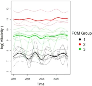
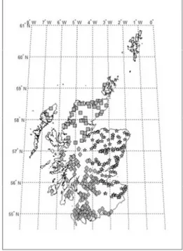
Using data provided by the Scottish Environment Protection Agency, Haggarty et al., (2012) studied a subset of monitoring data from of 24 lochs, comprising 7 pre identified groups covering the period 2003 – 2006, with three determinands, Alkalinity, Phosphorus, and Chlorophyll. Currently classification for the purposes of the WFD is based on a single representative loch, with groups based on typology (altitude, alkalinity, depth). The representative member is often determined by logistics. Figure 1 below shows the results from applying a functional clustering approach to these data. This resulted in the identification of 3 groups (as opposed to the 7 in use). The clusters differ in terms of the averages, seasonal patterns and also the intra-site variability.
Other examples in the literature where functional clustering has been applied to environmental data include (Henderson, 2006, Pastres et al., 2011, Ignaccolo et al., 2008). The power of this approach is in treating irregularly spaced time series as curves (and as a result we do not have to worry about matching dates). Computationally this can be very powerful and efficient, and recent work has extended this to include spatial correlations (Jiang and Serban, 2012). More recently, Haggarty (2012), has used this approach applied to a river network to identify clusters of locations incorporating an appropriate river network spatial correlation.
Figure 1 – Group curves and membership of 24 lochs based on alkalinity (Haggarty, 2012).
4.2 Flexible additive models for river networks
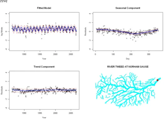
In the context of the WFD, one emphasis is on river networks, flexible additive models are another set of statistical tools that are gaining widespread use in the environmental setting, since they can be developed to examine the temporal and spatial trends and seasonality within e.g. a river catchment, to incorporate catchment covariates and to incorporate space/time interactions and an appropriate covariance structure for looking at water quality. The benefit of such an approach is the flexibility to model smooth trends in space and time along with flexible non-restricted seasonal patterns, improving knowledge of detailed changes across space and time. For a river catchment, we could anticipate that there would be several monitoring locations along the main channel and tributaries. This sounds like a very conventional spatial problem, but the natural structure of the river must be considered, points close in Euclidean space may be unconnected, so that interpolation over the entire network is possible, but needs a special spatial model. In particular, a river distance model (where river distance is defined as the shortest distance between two locations, and where connectedness of locations is considered along the river network) is useful. Work by Ver Hoef at al (2006) and Cressie et al. (2006) introduced river distance based models. Further work is ongoing developing such models. (O’Donnell, 2012, O’Donnell et al., 2014, Peterson et al., 2013).
Figure 2 shows the river Tweed network, again using monitoring data provided by SEPA. The data set included more than 80 monitoring stations on the river network, and a time series of approximately monthly frequency for more than 15 years. The circle represent one station on the network, and the individual panels show the overall fitted model, with the trend and seasonal components, fit using an additive model including a
rive
Figure 2 – Group Fitted additive model to the time series from a single site, but where the model has used a river distance covariance model (O’Donnell, 2012).
river distance correlation. Models such as these allow interpolation along the river network based on the relatively sparse sampling locations.
4.3 River flow and extremes
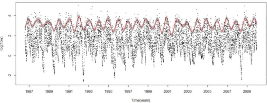
Floods and droughts are of major concern for those concerned with sustainable management of water which requires extreme value modelling. In the context of the Floods directive, European countries must prepare flood risk maps, so statistically, the most interesting question concerns the spatial pattern in extremes. This is also of considerable scientific interest in the wider context of climate change. Generalisation and extension from univariate extreme value theory is complex, with recent developments exploring max-stable stochastic processes and building spatial hierarchical statistical models (Fuentes et al., 2012) to answer questions about trends in extremes. Quantile regression approaches can also be used to explore the extremes or high quantiles in non-stationary time series. (Franco Villoria 2013) . In this work, non-parametric additive models, including seasonal and trend effects are fit to high quantiles, and then return levels and periods can be estimated. A 95th quantile regression model for the river Ness in Scotland can be seen in Figure 3. The data are accessed from the National River Flow Archive and are daily data for more than 30 years. This model (incorporating a trend+ seasonal component) allows for investigation of temporal changes in high quantiles of daily river
flow. The fitted model highlights the different seasonal patterns (troughs and peaks) over
Figure 3 – 95th quantile regression for daily river flows (Franco Villoria, 2013).
the observation period.
At the same time, a spatial quantile additive regression model can also be fit (Franco Villoria, 2013), and additional regional and global scale drivers such as NAO can be included as covariates.
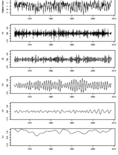
Additionally understanding the patterns of behaviour and variability is important. Wavelet analysis is a useful tool for analyzing non-stationarity or/and high frequency time series (Labat, 2005, 2010). The result is a time-scale decomposition of the original time series that allows cyclical components over different frequencies to be identified. Figure 4 below shows a wavelet decomposition of monthly maximum river flow for the river Tweed. This shows that the variability is not constant over time, and this can be linked to flood rich and flood poor periods in Scotland (Black &Burns, 2002). Each of the panels shows the variation at different temporal scales, and the final panel can be considered as the trend. Panel D3 relates to the seasonal pattern and shows how this varies over the observation period, with the total observation period broken into stretches of time when the amplitude of the signal is low, followed by periods with much greater oscillations.
4.4 Identification of common trends
In environmental and ecological sciences, the correlation or synchrony between major fluctuations in a set of time series is often described as temporal coherence (Livingstone, 2010, Finazzi et al., 2013). Statistical models are therefore needed which do not regard the individual time series separately but rather recognise that common drivers will impact at regional and sub-regional spatial scales. Classically the search for coherency has been done in a pairwise fashion, or using cross-wavelet coherency and phase, however modern approaches include the application of dynamic factor analysis, (Zuur et al., 2003,Finazzi et al., 2013) as an alternative, and recent developments have combined this with a clustering approach. Figure 5 shows preliminary results based on examining more than 300 time series of total organic carbon (TOC) values measured and reported approximately monthly in rivers in Scotland. Using the approach of Finazzi at al (2013), 3 clusters of
coherent time series were identified. The clusters were then mapped, and Figure 5 shows a
Figure 4 – Wavelet decomposition of river Tweed flow data (Franco Villoria, 2013).
clear spatial divide that can be linked to soil types and meteorology as drivers of regional patterns in TOC.
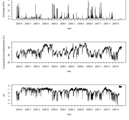
4.5 Events, events duration and their effects
In the final case study, the questions of scientific interest are a) identification of events (in this case extreme flows) in a river system, and b) how other determinands such as Dissolved Organic Carbon behave in response to such events. In this case, the data are collected automatically every 15 minutes, from a sensor system. This high temporal frequency of observation changes the nature of the statistical challenge, but more importantly changes the nature of ecological and biogeochemical questions that are asked (Kirchner et al., 2004). Relationships in terms of the mean response are no longer of primary interest but rather more transient relationships, driven by ‘events’ of short
duration are of interest, especially as they capture pulses of pollution. In this particular
Figure 5 – Clustering for Scottish rivers based on dynamic factor analysis (Finazzi et al., 2013).
case, we can combine a peak over threshold approach to flow to identify events discharge and thus identify the same periods in the pH and conductivity series to build models of the response of pH and conductivity to flow events (Hamzah, 2012). Figure 6 shows an example of the three determinands of flow, pH and conductivity over a 4 year period. This quite clearly shows the transient nature of events in flow, and the complex nature of the relationship with the response in pH, and conductivity. Statistical tools and models to link such time series together are needed to identify the nature of the relationships and the scales at which they operate (Kirchner, 2006, Neal et al. 2012).
5.
SENSORS AND SENSORS NETWORKS - THE FUTURE
Sensing and making sense of the environment (whether natural or urban) in the 21st century will be based round sensor networks “Sensor networks will produce a revolution in our understanding of the environment by providing observations at temporal and spatial scales that are not currently possible. Expanding observational scales will enable a deeper and broader understanding of environmental variability and change that will, in turn, improve public awareness, enabling better informed public policies and addressing the intrinsic interdependence of human society and the natural environment.” (NSF, 2004). The climate change research agenda is just one example (albeit a critical one) of the mathematical and statistical elements relevant to a more general “sensing of the natural environment” theme. National and international environmental policy setting and
Figure 6 – Coupled 15 minute environmental time series of river discharge, conductivity and pH (Hamzah, 2012).
evaluation requires a strong and robust evidence base. The key to the delivery of this deeper and broader understanding is the development of spatio-temporal modelling able to handle uncertainty, be computationally robust (and able to deal with “big data”), to accommodate time-varying (non stationary) spatial processes where the data come from multiple sources, to have an appropriate inferential framework and which can deliver visualisation tools.
In addition, such capability will ensure risk informed decision making, in application areas such as monitoring of impacts with regard to renewable energy developments, security (in an urban environment), water resources (floods, droughts, quality and quantity), and carbon budgets. Global environmental monitoring from satellites through to more local environmental monitoring such as probes in individual water courses measuring water quality, sediment transport and pollutant concentrations, will change the landscape of the environmental statistician and how we see our world. Environmental sensor networks will become the standard research tool for earth and environmental sciences (Rundel et al., 2009), and Statistics and statisticians are in a strong position to lead and contribute to this movement.
As our knowledge of environmental systems grows so will our understanding of their complexity, thus spawning a next generation of environmental research questions. These few, brief case studies, highlight the nature of the environmental questions and the statistical modelling approaches being used to examine the temporal and spatial trends and
seasonality, to incorporate important covariates and space/time interactions and appropriate covariance structure for the environmental context.
Appropriate and exciting statistical modelling helps explore and understand patterns in the data, integrate and synthesise observations from a variety of networks, investigate changes, estimate and predict statistics is a key tool to deliver the evidence base on impact and change and for data transformation.
ACKNOWLEDGEMENTS
NERC KE AWARD, “ENVIRONMENT, REGULATION AND STATISTICS”, NERC CONSORTIUM AWARD “GLOBOLAKES”, NERC VALUING NATURE NETWORK “INQUEST”.
Our colleagues, PhD and MSc students at Glasgow University: Adrian Bowman, Claire Miller, Ruth Haggarty (for Figure 1), David O’Donnell (for Figure 2), Maria Franco-Villoria (for Figures 3,4). Alastair Rushworth, Susan Waldron and Firdaus Hamzah (for Figure 6). Our colleagues at Scottish Environment Protection Agency : Mark Hallard, Fiona Wylie, Malcolm Smith. Our colleagues in Italy: Daniela Cocchi, Massimo Ventrucci, Francesco Finazzi (for Figure 5), Alessandro Fasso. This paper is based on an invited presentation given at METMA6 in Guimaeraes in September 2012.
REFERENCES
R. BARANIUK (2011). More Is Less: Signal Processing and the Data Deluge. Science, 331, no. 11, pp. 717-719, February.
V. BARNETT, A. O’HAGAN (1997). Setting environmental standards: The statistical approach to handling uncertainty and variation. London, Chapman & Hall.
A. BLACK, C. BURNS (2002). Re-assessing flood risk in Scotland. Science of the Total Envi-ronment, 294, pp. 169-184.
CCRA (2012). http://www.defra.gov.uk/publications/2012/01/26/pb13698 climate change-riskassessment/.
N. CRESSIE, J. FREY, B. HARCH, M. SMITH (2006). Spatial prediction on a river network. Journal of Agricultural, Biological and Environmental Statistics, 11, no. 2, pp. 127-150.
EC WATER FRAMEWORK DIRECTIVE (2000). "Directive 2000/60/EC of the European Parlia-ment and of the Council establishing a framework for the Community action in the field of wa-ter policy" downloaded April 2010 from EC/Environment web site.
EC FLOODS DIRECTIVE http://register.consilium.europa.eu/pdf/en/07/st03/ st03618.en07.pdf downloaded October 2011.
F. FINAZZI, M. SCOTT, C. MILLER, A. FASSO (2013). A model-based clustering approach for the study of the temporal coherence of multivariate time series. Submitted Annals of Ap-plied Statistics.
M. FUENTES, J. HENRY, B. REICH (2012). Nonparametric spatial models for extremes: appli-cation to extreme temperature data. Extremes, 127.
M. FRANCO VILLORIA (2013). Temporal and spatial modelling of extreme river flow values in Scotland. PhD thesis, University of Glasgow.
J. C GEMMELL, E. M. SCOTT (2013). Environmental regulation, sustainability and risk. Sus-tainability, Accounting, Management and Policy (in press).
P. GUTTORP (2006). Setting environmental standards: a statistician’s perspective. Environ-mental Geosciences, 13, no. 4 (December 2006), pp. 261–266.
R. HAGGARTY (2012). Evaluation of sampling and monitoring designs for water quality. PhD thesis, University of Glasgow
R. A. HAGGARTY, C. MILLER, E. M. SCOTT, F. WYLLIE, M. SMITH (2012). Functional clus-tering of water quality data in Scotland. Environmetrics, 23, no. 8, pp. 685-695.
F. M. HAMZAH (2012). Statistical Analysis of freshwater parameters monitored at different temporal resolutions. PhD thesis, University of Glasgow
R. IGNACCOLO, S. GHIGO, E. GIOVENALI (2008). Analysis of air quality monitoring net-works by functional clustering. Environmetrics, 19, no. 7, pp. 672–686.
IPCC (2008). Technical paper on climate change and water. http://www.ipcc.ch/pdf/tecni cal-papers/climate-change-water-en.pdf J. KIRCHNER, X. FENG, C. NEAL, A. ROBSON (2004). The fine structure of water-quality
dynamics: the (high-frequency) wave of the future. Hydrological Processes, 18, pp. 1353-1359.
J.W KIRCHNER (2006). Getting the right answers for the right reasons: linking measure-ments, analyses, and models to advance the science of hydrology. Water Resources Re-search, 42.
D. LABAT (2005). Recent advances in wavelet analyses: Part 1. A review of concepts. Journal of Hydrology 314, pp. 275-288.
D. LABAT (2010). Cross wavelet analyses of annual continental freshwater discharge and se-lected climate indices. Journal of Hydrology 385, pp. 269-278.
D. M. LIVINGSTONE, R. ADRIAN, L. ARVOLA, T. BLENCKNER, M. DOKULIL, R. HARI, G. GEORGE, T. JANKOWSKI, M. JARVINEN, E. JENNINGS, P. NOGES, T. NOGES, D. STRAILE, G WEYHENMEYER (2010).Regional and supra-regional Coherence in limnological
variables. In GLEN GEORGE (eds.), The impact of climate change on European lakes, Spring-er, pp. 311-337.
MEA (2005). http://www.unep.org/maweb/en/index.aspx NEA (2011). http://uknea.unep-wcmc.org/Resources/
C. NEAL, B. REYNOLDS, P. ROWLANDS, D. NORRIS, J. W. KIRCHNER, M. NEAL, D. SLEEP, A. LAWLOR, C. WOODS, C. THACKER, H. GUYATT, C. VINCENT, K. HOCKENHULL, H. WICKHAM, S. HARMAN, L. ARMSTRONG (2012). High frequency water quality time series in precipitation and stream flow: from fragmentary signals to environmental chal-lenge. Science of the Total Environment, 434, pp. 3-12.
D. O'DONNELL, A. RUSHWORTH, A. BOWMAN, M. SCOTT, M. HALLARD (2014). Flexible regression models over river networks. Journal of the Royal Statistical Society series A, 63(1), 1-17
D. O’DONNELL (2012). Spatial Prediction and Spatio-Temporal Modelling on River Net-works. PhD thesis, University of Glasgow
R. PASTRES, A. PASTORE, S. F. TONELLATO (2011).Looking for similar patterns among moni-toring Stations. Venice lagoon application. Environmetrics, 22, no. 6, pp. 712–724.
E. PETERSON, J. VER HOEF, D. ISAAK, J. FALKE, M. FORTIN, C. JORDAN, K. MCNYSET, P. MONESTIEZ, A. RUESCH, A. SENGUPTA, N. SOM, A. STEEL, D. THEOBALD, C. TORGERSEN, S. WENGER (2013).Modelling dendritic ecological networks in space: an inte-grated network perspective. Ecology Letters, doi: 10.1111/ele.12084
P. W. RUNDEL, E. A. GRAHAM, M. F. ALLEN, J. C. FISHER, T. C. HARMON (2009). Envi-ronmental sensor networks in ecological research. New Phytologist, 182, no. 3, pp. 589–607.
E. M. SCOTT, J. C. GEMMELL (2013). Water quality assessment and European Water Framework Directive. Encyclopaedia of Environmetric, 2nd edition, Wiley.
E. M.SCOTT, J. C. GEMMELL (2012). Spatial Statistics- a watery business. Spatial Statistics, 1. R.I. SMITH, J. MCP. DICK, E. M. SCOTT (2011). The role of statistics in the analysis of ecosystem
services. Environmetrics, 22, no. 5, pp. 608-617.
J. M. VER HOEF, E. PETERSON, D. THEOBALD (2006). Spatial statistical models that use flow and stream distance. Environmental and Ecological Statistics, 13, no. 4, pp. 449-464.
A.F.ZUUR,R.J.FRYER,I.T.JOLIFFE,R.DEKKER,J.J.BEUKEMA (2003).Estimating common trends in multivariate time series using dynamic factor analysis. Environmetrics, 14, pp. 665-685.
SUMMARY
Assessing, valuing and protecting our environment- is there a statistical challenge to be answered?
This short article describes some of the evolution in environmental regulation, management and monitoring and the information needs, closely aligned to the statistical challenges to deliver the evidence base for change and effect.