DECOMPOSITION OF VARIANCE IN TERMS OF CONDITIONAL MEANS
A. Figà Talamanca, A. Guerriero, A. Leone, G. P. Mignoli, E. Rogora
1. INTRODUCTION AND METHODOLOGY
Let X =( ,x1 …,xN) be a numerical variable defined on a population P of N individuals. We may think of X as an element of a real vector space L of dimen-sion N. We equip L with a real, normalized scalar product: for ,X Y ∈L , and
1 ( , , N) Y = y … y , we define: 1 1 , N i i. i X Y x y N = < >=
∑
The length or norm of a vector is defined in terms of the scalar product: 2
, .
X =<X X >
The mean value of a vector X is of course the scalar
1 1 . N i i X x N = =
∑
We may also think of the mean value as a vector E X of L having all its 0( ) components equal to the scalar X . In this context E may be thought of as a 0 linear operator defined on L and mapping L into the subspace of constant vec-tors. The variance of X can be written then as:
2
0 0 0
( ) ( ) ( ), ( ) .
V X = X E X− =<X E X X E X− − >
We now suppose that the indices i= …1, ,N, correspond to individuals of a population P, and that X is a numerical variable defined on the population P. We
1, ,2 , q
P P … P . Denote by P the number of elements of j P , so that j
1 q
N = P + + P . We can then define a vector E Xπ( ) with components: 1 ( ) ( ). k i j k j P k E X x i P P π ∈ =
∑
∈ (1)Observe that two components of this vector are identical if their indices be-long to the same class Pk of the partition π. The trivial identity:
0( ) ( ) 0( ) ( ), X E X− =E Xπ −E X +X E X− π implies 2 2 2 0 0 ( ) ( ) ( ) ( ) ( ) , V X = X E X− = E Xπ −E X + X E X− π
because, as it is easily seen, E Xπ( )−E X0( ) and X E X− π( ) are orthogonal
vectors.
Suppose now that π π1, 2,…,πn is a finite sequence of partitions of the popu-lation P, into respectively q q1, ,2 …,qn, classes. Suppose further that each parti-tion πj is a refinement of the partition πj−1. (This means that each class of the partition πj is contained in a class of the partition πj−1). Define for complete-ness the trivial partition π0 consisting of the full population P. Let j
k
P , for
1, , j
k= … q be the disjoint classes of the population P relative to the partition j
π . With reference to the partition πj define the operator
( ) j( ) .
j
E X =Eπ X
In this fashion (1) reads: 1 ( ) , ( ). j j k j i j h k h P k E X x i P P π ∈ =
∑
∈Observe that this definition makes sense also in the case j = 0. The trivial iden-tity 0 1 1 ( ) n [ j( ) j ( )] n( ) . j X E X E X E − X X E X = − =
∑
− + − (2)2 2 1 1 ( ) n j( ) j ( ) n( ) . j V X E X E − X X E X = =
∑
− + − (3)We are interested in the case in which the sequence of partitions πj is defined by a sequence of qualitative characters C C1, 2, ,…Cn of the population P. We can define the partition πj by considering the classes of the population formed by individuals with identical values of the first j characters.
In this case the first n summands on the right hand side of (3) represent the contributions to the variance of the n qualitative characters C1, ,…Cn within the population considered.
Observe however that, while the sum of the first n terms of the right hand side of (3) is independent of the order in which the characters C1, ,…Cn are consid-ered, the operators E , for 0< j < n are defined with respect to partitions which j
strongly depend on the order in which the characters are taken. As an obvious consequence, the value of each term E Xj( )−Ej−1( )X 2 also depends on the order of the characters. In a different order the characters would define a differ-ent set of partitions; only π0 and πn, and consequently E and 0 E are inde-n pendent of the chosen order.
We are led therefore to look for a natural order of the qualitative characters considered. We propose an ordering based on systematic, step by step, compari-sons of the conditional means with respect to the variables considered. This or-dering, which we call Stepwise Optimal Ordering (SOO) is defined as follows:
We choose the character C and the corresponding partition 1 π1 which maxi-mizes E X1( )−E X0( )2. If C1, ,… Ck are chosen, the character Ck+1 is chosen so that it refines the partition πk into the partition πk+1 in such a way that the value Ek+1( )X −E Xk( )2 is largest.
The order C1, ,… Cn determined in this fashion may be considered as a rank-ing of the variables. One should be aware, however, that this rankrank-ing cannot be interpreted in terms of relative importance in determining the phenomenon measured by the variable X. As will be seen in the applications below, the qualita-tive characters considered may be far from independent. This may imply that a character which is recognized as a primary cause of the intensity of the phe-nomenon measured by X, may be mediated by other characters to whom it is as-sociated, and therefore appear in the last positions of the ranking.
We do not propose a clear cut interpretation of the significance of the ranking obtained by our method, nor of the relative size of the first n addends which ap-pear in (3), when the qualitative characters are ordered according to our prescrip-tion. On the contrary, rather than expecting straight answers, we expect that both
the ranking and the relative size of the addends in the expression (3) would solicit questions concerning the dependence of the variable X on the qualitative vari-ables and the interdependence of the qualitative varivari-ables themselves (with all the cautions regarding the possibility to consider causal relations between the vari-ables, (Blalock, 1961; Sobel, 1996; Sobel, 1998; Sobel, 2000).
Nevertheless, in the very special case considered in the simulated experiment of section 4, our method yields a ranking that reflects the relative weight of the characters.
In the following two sections we apply our method and discuss the “ranking” of the qualitative characters, thus obtained to two sets of data. The fourth section is dedicated to a simulated experiment.
We should mention that the ideas contained in chapter 8D of Diaconis (1988) were influential in the inception of this work, which started as an attempt to apply Diaconis' ideas to the case of tree-structured data, under the action of the group of tree-automorphisms. Under this action the ranges of the operators Ej −Ej−1 turn out to be irreducible subspaces of L.
2. THE SCORE ON AN ENTRANCE EXAMINATION
Entering students of the University of Rome “La Sapienza” in scientific and technical fields take a multiple choice test in mathematics, which consists of 30 questions1. At the moment the purpose of the test is to discourage students who do not have an adequate background, and to make students aware of their poten-tial weaknesses.
We consider a population of 2,451 students who took the test in 2005, and we let X be the score achieved by each student, that is the number of correct answers. The variable X depends on the 30 dyadic characters, corresponding to the correct or incorrect answer to each question. Of course, in this case,
30( ) E X =X , and 30 2 2 0 1 1 ( ) ( ) j( ) j ( ) . j V X X E X E X E − X = = − =
∑
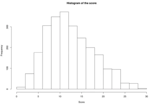
−The variable X takes values between 0 and 30. Its mean value is 12.9 and the variance is ( ) 29.8V X = . The histogram of X is in Fig. 1.
1 The test, in Italian, is available for downloading at the internet address http://www.mat.
Figure 1 – The histogram of the score.
An application of our method shows that just ten questions, chosen according to the ranking we propose, “explain” 88% of the variance. In other words, if we write 10 2 2 1 10 1 ( ) j( ) j ( ) . j V X E X E − X X E = =
∑
− + −the remainder term X E− 10 2=3.58 amounts to just 12% of ( ) 29.8V X = . We presently list the remainders X E− k 2, for k = …1, ,10, obtained by applying our method, as percentage of ( )V X . To wit the values
2 / ( ) k k c = X E− V X , 1 2 3 4 5 6 7 8 9 10 75 , 59 , 48 , 40 , 34 , 100 100 100 100 100 29 , 25 , 20 , 16 , 12 . 100 100 100 100 100 c c c c c c c c c c = = = = = = = = = =
We do not claim that our method necessarily chooses the 10 characters for which X E X− 10( )2 is lowest. In general, with arbitrary data, this may not be the case.
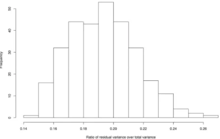
However, in this particular case, our choice compares well with other possible choices, as shown by the experiment which we presently describe. We selected, at random, 300 subsets of ten elements of the original thirty questions and we com-puted the conditional mean E Xπ( ) with respect to the partition π obtained by grouping together the students with identical performance on each of the ten question chosen. We computed then
2 ( ) ,
X E X− π (4)
relative to each “ten element” choice. The results are summarized in Fig. 2.
Figure 2 – Histogram of the values of residual variance (4), as percentage of total variance for 300 randomly selected subsets of 10 questions.
Observe that the lowest value of quantity (4) achieved by one of the 300 sub-sets we selected, is higher than 0.14, while with the SOO choice of ten characters we achieved the value 0.12.
The experiment shows that the algorithm we propose performs decidedly bet-ter than a random choice if we want to choose ten out of thirty questions, in such a way that the total variance of the variable X is best explained. In conclusion there is at least some experimental evidence that our method may be used to se-lect a small number of characters which account for most of the variance.
The variables selected according to SOO discriminate the students better than the other variables, Indeed, if we rank the items according to the item discrimina-tion index of classical test theory, the ten items selected by SOO find place among the first 11 items. We also estimated, according to Rasch model, the diffi-culty of the 30 items. It turns out that the ten items chosen according to SOO occupy a middle position. Indeed the 10 items thus chosen place themselves
be-tween the eight and the twentieth position in the ranking. Finally, we note that eight of the ten selected variables are among the ten most important variables in terms of linear regression and the order of the first five variables coincides under both methods.
3. THE VARIABLE “DELAY IN COMPLETING A DEGREE”
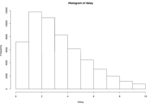
The Italian system of higher education is characterized by the marked differ-ence between the time employed by most students to complete a degree and the number of years formally required to graduate. The average delay in completing a degree is well above two years for most fields of study2. In this section we con-sider a population of Italian university graduates obtained using the data bank “AlmaLaurea” which collects data of university graduates from a set of Italian universities3. The population amounts to 58,091 graduates of 27 universities in 2003. On this population the variable X represents the delay in completing the degree, computed in years, starting from a conventional date (November 1st) in which according to formal regulations the degree should have been completed. We excluded delays above ten years, which should be better interpreted as leaving and resuming the studies after several years. We study the dependence of X on seven possible characters, which are the following:
(UN) University where the degree was obtained (PE) Parent's level of education
(HS) Type of high school attended (GD) Grade in the final year of high school
(MA) Degree major
(WO) Working or not working during the studies (GN) Gender
Proceeding as outlined in the introduction, we obtain the following ranking of the seven variables:
GD, UN, MA, HS, PE, WO, GN. Accordingly we consider the operators
0, 1, 2, 3, 4, 5, 6, 7, E E E E E E E E
and write
2 The recent reform of the university system may hopefully change this in the near future. 3 AlmaLaurea Consortium is an association of 49 Italian universities which, since 1994 collects
statistical data about the scholastic and employment records of university graduates (Cammelli, 2005; Cammelli, 2006). The data bank of AlmaLaurea is also made available, under certain condi-tions, to prospective employers.
7 2 2 1 7 1 ( ) j( ) j ( ) ( ) j V X E X E − X X E X = =
∑
− + − (5)The variance of the variable X is V(X)=4.61, while the residual variance, not “explained” by the qualitative variables under consideration is
2
7( ) 1.94
X E X− = . The decomposition of the variance (3) is:
4.61 (0.30 0.28 0.49 0.45 0.51 0.33 0.31) 1.94 2.67 1.94= + + + + + + + = +
Thus 2.67 represents the portion of the variance which is “explained” by the characters considered. We may say, therefore, that these characters explain 62% of the variance.
In this case the ranking obtained by our method is relatively “robust”. Indeed if we omit consideration of one of the characters, the relative ranking of the other characters remains unchanged. We do not claim of course that this type of “ro-bustness” is inherent in our method. It may very well occur, with different data, that omitting one character would determine a change in the order of the remain-ing ones.
We compared our results with those obtained by using the binomial logistic re-gression and the multivariate analysis of variance. Notice, however, that these methods, unlike SOO, require hypothesis on the distribution of data which are not met by our example. On the other hand, SOO is not suitable for inferential purposes.
As for the binomial logistic regression, the response variable was dichotomized assigning the value zero to the population of graduates with a delay of less than one year (34.1%) and value one to the others (65.9%). This is of course an arbi-trary choice, which has to be made to apply the method. As a measure of the ef-fect produced by each independent variable we use the standard deviation of the theoretic probabilities associated to the values of the independent variables4. The results of our computations are summarized in table 1.
TABLE 1
Effect of the 7 independent variables on the probability to graduate within one year logistic binomial regression analysis
Variable SOO Effect
GD 1 0.11 UN 2 0.09 MA 3 0.10 HS 4 0.06 PE 5 0.04 WO 6 0.03 GN 7 0.01
4 More precisely, let p(j,i) be the mean of the probabilities of graduating within one year after
forcing, in our population, the j variable to take the value i. The effect of the variable j is then de-fined to be the standard deviation of the numbers p(j,i), weighted by the numbers n(j,i) of individu-als for which the j-th variable takes the value i in the original population.
We observe that the ranking of the variables determined by the effects on the dependent variable coincides, except for one inversion, with the ranking obtained by SOO. It should be noted that in the regression model we inserted only the principal effects of the independent variables and not the possible interaction be-tween them.
The comparison of SOO with multivariate analysis of variance yields almost exactly the same results.
Figure 3 – Histogram of the delay.
4. A SIMULATED EXPERIMENT
In order to better understand the properties of our Stepwise Optimal Order, we performed a simulation, repeating 20 times the following experiment.
First we constructed 10 vectors x1, ,… x10 each of 100 components and each component extracted from a simulated Bernoulli variable. Then we considered the variable
1 1 2 2 10 10
x c x= +c x + +c x + (6) ε
with c1=1,c2=0.9, ,… c10 =0.1 and ε consisting of 100 independent realizations of a simulated Gaussian variable with mean 0 and standard deviation 0.03.
In 18 cases out of the 20 observed experiments, SOO was exactly 1, 2, 3, ..., 10, i.e. for the variable x this order reflected, most of the time, the size of the
co-efficients c1, ,… c10 which enter formula (6). In the remaining two cases the dif-ference between SOO and the increasing order was just one inversion.
5. CONCLUSIONS
We conclude that the application of our method to numerical variables which depend on qualitative variables, may yield valuable information and insights on the dependence of the numerical variable on the qualitative variables, and the in-terdependence of the qualitative variables themselves. We observe that in the simulated experiment described in the last section the ranking obtained by our method reflects the relative weight of the variables. Nevertheless we do not pro-pose, in general, a clear cut interpretation of the significance of this ranking. Fi-nally we observe that the role of the qualitative variables in the two sets of data on which we test our method is different. In the first example the 30 variables are measures of the response variable, rather than causes of it, while in the second example the qualitative variables may be interpreted as “causes” of the numerical variable and the interpretation of the results may very well be different.
Department of Mathematics ALESSANDRO FIGÀ TALAMANCA
University of Rome “La Sapienza”
Alma Laurea ANGELO GUERRIERO
ALBERTO LEONE GIAN PIERO MIGNOLI
Department of Mathematics ENRICO ROGORA
University of Rome “La Sapienza”, [email protected]
REFERENCES
H.M.JR. BLALOCK,(1961), Causal inferences in Nonexperimental Research, Chapel Hill, Univerity of North Carolina Press, 1961.
A. CAMMELLI, (2005), La qualità del capitale umano dell'università. Caratteristiche e per-formance dei laureati 2003, in La qualità del capitale umano dell'università in Europa e in
Italia, ed. Cammelli A., Bologna, Il Mulino, 2005.
A. CAMMELLI, (2006), La riforma alla prova dei fatti, in Settimo profilo dei laureati italiani, ed. Consorzio interuniversitario AlmaLaurea, Bologna, Il Mulino, 2006.
P. DIACONIS, (1988), Group Representations in Probability and Statistics, Lecture notes - Mono-graph series volume 11, Institute of Mathematical Statistics, Hayward, California, 1988. M.E. SOBEL,(1996), An Introduction to Causal Inference, in Sociological Methods and Research,
24, 1996, pp. 353-379.
M.E. SOBEL,(1998),Causal Inference in Statistical Models of the Process of Socioeconomic Achievement, in Sociological Methods and Research, 27, 1998, pp. 318-348.
M.E. SOBEL,(2000),Causal Inference in the Social Sciences, in Journal of the American
SUMMARY
Decomposition of variance in terms of conditional means
Two different sets of data are used to test an apparently new approach to the analysis of the variance of a numerical variable which depends on qualitative variables. We suggest that this approach be used to complement other existing techniques to study the interde-pendence of the variables involved. According to our method, the variance is expressed as a sum of orthogonal components, obtained as differences of conditional means, with re-spect to the qualitative characters. The resulting expression for the variance depends on the ordering in which the characters are considered. We suggest an algorithm which leads to an ordering which is deemed natural. The first set of data concerns the score achieved by a population of students on an entrance examination based on a multiple choice test with 30 questions. In this case the qualitative characters are dyadic and correspond to cor-rect or incorcor-rect answer to each question. The second set of data concerns the delay to obtain the degree for a population of graduates of Italian universities. The variance in this case is analyzed with respect to a set of seven specific qualitative characters of the popula-tion studied (gender, previous educapopula-tion, working condipopula-tion, parent's educapopula-tional level, field of study, etc.)