Polychaete fauna of the Northwest Portuguese Coastal Shelf: ecology, diversity and distribution

1

ALMA MATER STUDIORUM

UNIVERSITÀ DI BOLOGNA

SCUOLA DI SCIENZE - CAMPUS DI RAVENNA

CORSO DI LAUREA MAGISTRALE IN BIOLOGIA MARINA

Polychaete fauna of the Northwest Portuguese

Coastal Shelf: ecology, diversity and distribution

Tesi di laurea in Alterazione e Conservazione degli Habitat Marini

Relatore Presentata da

Prof. Marco Abbiati Serena Mucciolo

Correlatore

Prof. Victor Quintino

II sessione

2

INDEX

1- INTRODUCTION ... 3

1.1- Importance of polychaete fauna ... 3

1.2- Description of the study area ... 5

1.3- Aims of the work ... 9

2- MATERIAL AND METHODS ... 10

2.1- Field work ... 10

2.2- Laboratory work ... 11

2.3- Data analysis ... 13

3 - RESULTS ... 15

3.1- Data analysis ... 15

3.2- Description of selected families ... 24

4 - DISCUSSION AND CONCLUSION ... 39

3

1- INTRODUCTION

1.1- Importance of polychaete fauna

Polychaetes are one of the most abundant macroinvertebrates with more than 9000 species recognised (Rouse and Pleijel 2001). Most are comprised in the macrofauna, but there are some species belonging to the families Saccocirridae and Syllidae, included in the interstitial fauna. As Surugiu et al., (2015) stressed, the extremely wide ecological adaptations of the polychaetes contributed to their ability to colonise all benthic habitats. Their high population densities gives them a leading functional role in all benthic communities.

Macrobenthic polychaetes play an important role in the marine food chain and are are used to assess the ecological status of benthic communities (Cacabelos et al., 2008; Lourido et al., 2008; Quiroz-Martinez et al., 2011). In fact, they represent one of the main trophic resources for the fish fauna, thus having an indirect importance for human economy. Polychaetes are characterized by a relatively high caloric content, being integrally ingested and digested (undigested remains of their bodies are only the cuticle, seta, jaws and paragnaths); so, both pelagic larvae and adults, are consumed from the planktophagic and benthofagic fishes (Surugiu et al., 2015). The exploitation derived by using them as a bait or food for aquacultured species is considerable and the Portuguese legislation (Portaria nº1102-B/2000) permits exclusively the harvesting of Marphysa sanguinea (Montagu, 1815), Diopatra neapolitana Delle Chiaje, 1841 and Nereis diversicolor O.F.Müller, 1776. Although legislation exists, control of the catch and policies to exploit baitworm stock in a sustainable way such as progressive exploitation of areas alternating with periods of recovery, is not in evidence (Costa et al., 2006).

Other polychaetes, as burrowing ones, are considered relevant ecosystem engineers (Gutiérrez & Jones, 2006; Volkenborn & Reise, 2006; Herringshaw et al., 2010) thanks to the capability

4

of some families, e.g. Sabellariidae and Serpulidae, to build calcareous and sediment structures. Furthermore, bioturbation, as a result of feeding, gallery construction, ventilation, may influence and create a complex mosaic of micro- and macro- environments important for the control of ecosystem functioning (Pischedda et al., 2008).

Polychaetes are also commonly the first colonizers of impacted marine sediments (Grassle & Grassle, 1974; Shull, 1997) and are considered among the taxa with the highest level of sensitivity to perturbation of the soft substrata (Markert et al., 2004). The presence, absence or relative biomass of specific polychaetes in marine sediments may provide an excellent indication on the condition or health of the benthic environment (Leal, 2013).

5 1.2- Description of the study area

Portuguese continental shelf, as described by Martins et al., (2012a), is comprised in the Atlantic Iberian Margin and extends from the Gulf of Cadiz to the Galicia Bank for approximately 900 km in length, with an average width of about 45 km and an irregular steep slope plunging to the abyssal plain. Shelf-break slope occurs approximately at 160 m depth; shelf is incised by several deep submarine canyons with a northeast-southwest trend. The three principals ones Nazaré, Setúbal and S. Vicente divide the Portuguese shelf into four main sectors: northwestern (Caminha-Nazaré), central (Nazaré-Setúbal), southwestern (Setúbal – Cape S. Vicente) and southern (Algarve, Cape S. Vicente – Vila Real St. António) (Vanney & Mougenot, 1990).

In general, most soft-bottom marine sediments include components from different origins: lithogenic, composed by detrital particles derived from weathering of continental rocks; biogenic consisting of skeletal remains and a hydrogenous or authigenic component (clays, ferromanganese oxyhydroxides), precipitated from seawater or through microbial activity (Schulz & Zabel, 2006).

The study area of this work goes from Ovar (40°55’ N) to Mondego Estuary (40°03’N), covering an area of around 5665 km² from 20 m to 150 m of depth, and is comprised in the first sector, the northwestern. In this sector, the continental shelf is moderately wide (30-60 km) and receives a significant sedimentary input from several rivers (Minho, Lima, Cávado, Ave, Douro, Vouga and Mondego), with highest fluvial discharges in the winter season (Alveirinho Dias & Nittrouer, 1984). The Douro River is responsible for 79% of the total annual shelf sediment supply, estimated in 2.25 x 106 t.y-1 (Oliveira et al., 1982).

In terms of hydrodynamic regime, Portuguese coast was divided by Bettencourt et al., (2004) into: exposed, moderately exposed and sheltered areas. This study area is comprised in the exposed area and is characterized by an extremely energetic regime of waves and tides and a complex current system (Fiúza et al., 1982).

6

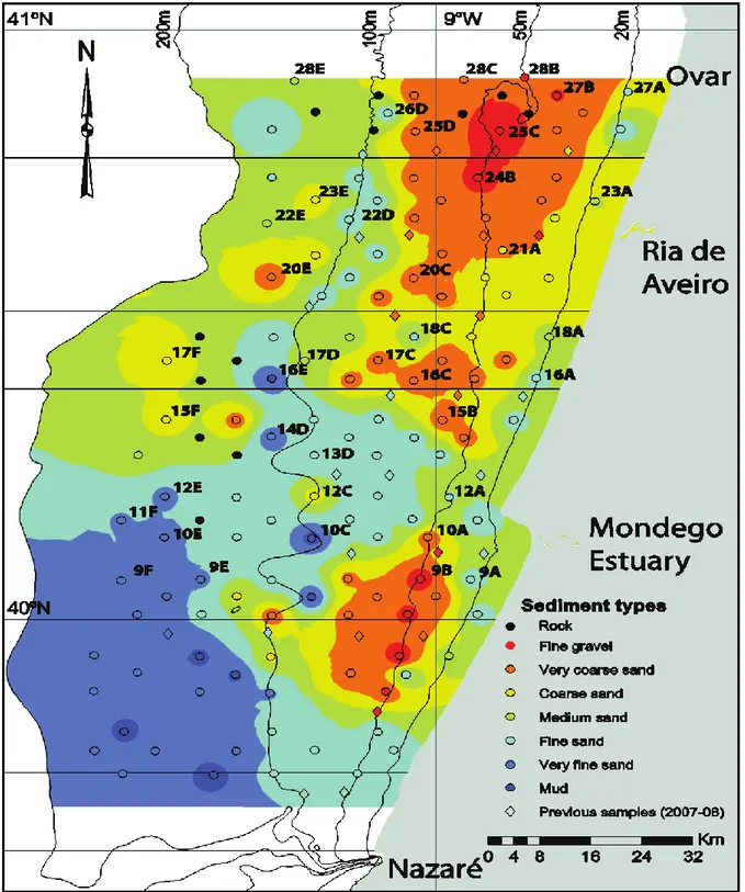
Martins et al., (2012a), and later Mamede et al., (2015), described in detail the grain-size of the Shelf following the Wentworth scale (Wentworth, 1922) for the textural classification. As showed in the figure 1.2, sampling sites were almost all covered by sand of different grain size; occasionally the muddy sediment was found. In table 1.2 data of the 39 sampling site are summarised, with relative coordinates, depth and grain size. Energetic regime, large fluvial sediment supply and the high total rainfall rates in the northern Portugal, may explain the spatial sediment distribution in the continental shelf. This area, in general, presents a high complex spatial sediment distribution with Mesozoic carbonated formations and discontinuous coarser deposit (ranging from gravel to coarse sand) mainly in the inner and mid-shelf between 20 and 80 m depth (Abrantes & Rocha, 2007); fine and very fine sand are found along a continuous band in the near shore shelf and in outer shelf of the northwestern sector (Martins et al., 2012).

7 Figure 1.2 Study area showing the position of each sampling site and the sediment types. Original

figure taken by Mamede et al., 2015 and modified adding labels of the 39 sampling sites investigated.

8

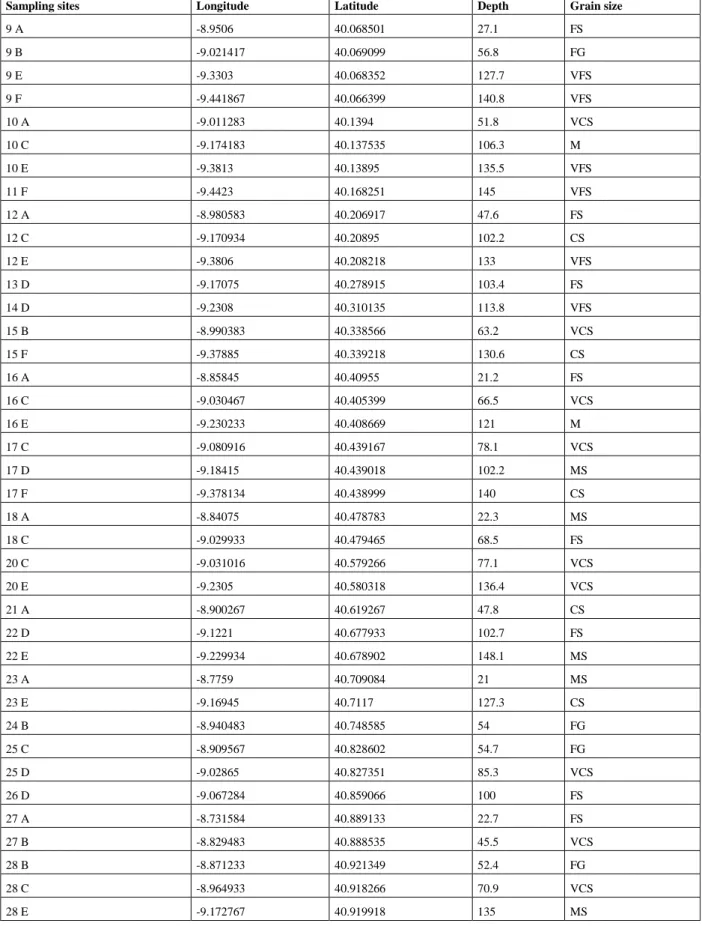
Sampling sites Longitude Latitude Depth Grain size

9 A -8.9506 40.068501 27.1 FS 9 B -9.021417 40.069099 56.8 FG 9 E -9.3303 40.068352 127.7 VFS 9 F -9.441867 40.066399 140.8 VFS 10 A -9.011283 40.1394 51.8 VCS 10 C -9.174183 40.137535 106.3 M 10 E -9.3813 40.13895 135.5 VFS 11 F -9.4423 40.168251 145 VFS 12 A -8.980583 40.206917 47.6 FS 12 C -9.170934 40.20895 102.2 CS 12 E -9.3806 40.208218 133 VFS 13 D -9.17075 40.278915 103.4 FS 14 D -9.2308 40.310135 113.8 VFS 15 B -8.990383 40.338566 63.2 VCS 15 F -9.37885 40.339218 130.6 CS 16 A -8.85845 40.40955 21.2 FS 16 C -9.030467 40.405399 66.5 VCS 16 E -9.230233 40.408669 121 M 17 C -9.080916 40.439167 78.1 VCS 17 D -9.18415 40.439018 102.2 MS 17 F -9.378134 40.438999 140 CS 18 A -8.84075 40.478783 22.3 MS 18 C -9.029933 40.479465 68.5 FS 20 C -9.031016 40.579266 77.1 VCS 20 E -9.2305 40.580318 136.4 VCS 21 A -8.900267 40.619267 47.8 CS 22 D -9.1221 40.677933 102.7 FS 22 E -9.229934 40.678902 148.1 MS 23 A -8.7759 40.709084 21 MS 23 E -9.16945 40.7117 127.3 CS 24 B -8.940483 40.748585 54 FG 25 C -8.909567 40.828602 54.7 FG 25 D -9.02865 40.827351 85.3 VCS 26 D -9.067284 40.859066 100 FS 27 A -8.731584 40.889133 22.7 FS 27 B -8.829483 40.888535 45.5 VCS 28 B -8.871233 40.921349 52.4 FG 28 C -8.964933 40.918266 70.9 VCS 28 E -9.172767 40.919918 135 MS

Table 1.2 Table of the sampling sites, their geographic coordinates, depth and grain size. Grain size: FG= fine gravel; VCS= very coarse sand; CS= coarse sand; MS= medium sand; FS= fine sand; VFS= very fine sand; M= mud.

9 1.3- Aims of the work

Despite the importance of polychaete fauna in characterising the structure and functioning of the benthic communities, the studies on most of the West Iberian coast are scarce and recent (e.g. Gil, 2011; Martins et al., 2013). This work was part of a wider research project that includes a comprehensive study of the benthic macrofauna communities from the Western and Southern Portuguese coastal shelf (Martins et al., 2012a; 2013a; 2013b) and their detailed spatial modelling in the Northwestern sector (Mamede et al., 2015). In this sense, the aim of this work is to investigate the composition and the spatial distribution of the polychaete fauna in a number of sites along this geographical sector; sampling was planned to cover the overall sedimentary grain-size gradient of this part of the costal shelf. Relationship to environmental factors were considered and the study added original data to the existing biological data set.

10

2- MATERIAL AND METHODS

2.1- Field work

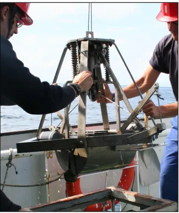
Samples were collected within the MeshAtlantic project (www.meshatlantic.eu, 24.10.2012), with which the Northern Portuguese Continental Shelf was sampled from Ovar – 41°0’ to Nazaré – 39°40’. A total of 121 sampling sites between 15 and 160 m of water depth and distanced each other no less than 5 km were taken along transects (Mamede et al., 2015). All the sediment samples were collected with a 0.1 m² Smith-McIntyre grab (fig. 2.1); a total of two samples were taken per site, one to study the macrofauna and the other to study the sediment descriptors (grain-size, total organic matter content and geochemistry analyses). Sediment samples were sieved on board over 1 mm mesh size and the macrofauna fixed in neutralized formalin (4%) stained with rose Bengal.

11 2.2- Laboratory work

The macrofauna samples were rinsed with water through a 0.5 mm mesh sieve under a fume hood and hand sorted. Following sorting, samples were fixed for long-term storage in 70% ethanol.

In this thesis 39 samples, distributed in the study area according to figure 1.2 were analysed. In these samples, polychaetes were the only group left to identify and 37, out of the 39 samples, were already sorted to the family level. For the taxonomic identifications the stereomicroscope Leica M205 C and the microscope Leica DMLB were used. The stereomicroscope was used to recognise the general and the “macro” features of each family and the microscope to examine the smallest details of each specimen, necessary for the species identification, e.g. chaetae, hooks and papillae.

The taxonomic identification up to the family level was carried out using Hayward & Ryland, (1995) and Rouse & Pleijel, ( 2001), as well as the DELTA database (Dallwitz et al., 2010) based on the interactive key Polikey (Glasby & Fauchald, 2003). For the taxonomic identifications to the species level several papers were consulted, as well as in-house laboratory keys and species description (tab. 2.2).

The validity and the authority of each species were confirmed in the World Register of Marine Species (WoRMS) (Read, 2015), and all the identifications were cross-checked by experienced colleagues from the same laboratory.

12 Table 2.2 Bibliography consulted for the taxonomic identifications up to species level. * denotes unpublished in-house species descriptions, notes and keys.

Family References

Acrocirridae Banse, 1969; Rouse & Pleijel, 2001 Ampharetidae Holthe, 1986

Amphinomidae Fauvel, 1923

Capitellidae Capaccioni-Azzati & Martin, 1992; Gravina & Somaschini, 1990; * Chaetopteridae Bhaud et al., 1994; *

Cirratulidae Chambers et al., 2011; de Kluijver et al., 2015; Unicomarine, 1996; * Dorvilleidae Jumars, 1974; *

Eunicidae Salazar-Vallejo & Carrera-Parra, 1998; Fauchald, 1992; Brito & Nunez, 2002; Nunez et al., 1997; *

Flabelligeridae Støp-Bowitz, 1948

Glyceridae O’Connor, 1987; Støp-Bowitz, 1941 Goniadidae Støp-Bowitz, 1941

Hesionidae VV.AA., 2004

Lumbrineridae Martins et al., 2012b; Oug, 2012 Magelonidae Fiege et al., 2000

Maldanidae Garwood, 2007 Nephtyidae Ravara, 2010

Nereididae Chambers & Garwood, 1992 Oenonidae Maron Ramos, 1973

Onuphidae Fauchald, 1982; Paxton, 1986; * Opheliidae Rowe, 2010

Orbiniidae Gil, 2011 Oweniidae Martin, 1989 Paralacydoniidae VV.AA., 2004

Paraonidae Aguirrezabalaga & Gil, 2009; Barwick, 2006; Blake, 1996; de Kluijver et al., 2015; Laubier & Ramos, 1973; Sardá et al., 2009; *

Pectinariidae Castelli & Valentini, 1995; Jirkov & Leontovich, 2013; Holthe, 1986 Phyllodocidae VV.AA., 2004

Pilargidae Katzmann et al., 1974; VV.AA., 2004 Poecilochaetidae Cantone, 1989; Pilato & Cantone, 1976 Polygordiidae Westheide, 1990

Polynoidae Barnich & Fiege, 2003; Fauvel, 1923; Pettibone, 1996 Sabellariidae Kirtley, 1994; *

Sabellidae Banse, 1979; Knight-Jones, 1983; Knight-Jones & Perkins, 1998; * Saccocirridae Westheide, 1990

Scalibregmatidae Worsfold, 2006 Serpulidae Zibrowius, 1968; *

Sigalionidae Barnich & Fiege, 2003; Martins et al., 2012c; VV.AA., 2004

Spionidae Bick et al., 2010; de Kluijver et al., 2015; Maciolek, 1985; Pardal et al., 1992; Pettibone, 1962

Sternaspidae Rouse & Pleijel, 2001 Syllidae San Martin, 2003 Terebellidae Holthe, 1986 Trichobranchidae Holthe, 1986

13 2.3- Data analysis

The abundance of all polychaetes and the species richness were calculated per sampling site. Abundance refers to the total quantity of specimens per sampling unit (0.1 m²); species richness (S), or alpha diversity () (Whittaker, 1960) corresponds to the number of species per sampling unit (0.1 m²). Other diversity indices were also calculated per site, namely, the Margalef richness (d), the Shannon-Wiener diversity (H’), the Pielou evenness (J’), and Simpson diversity (1-λ’).

The Margalef richness index (d) (Margalef, 1958) is the ratio between the number of the species and the number of specimens in a sample. It is given by 𝑑 = (𝑆 − 1)/ln⁡(𝑁) where, S is the number of the species found in the sample and N is the total number of specimens of that sample.

The Shannon-Wiener diversity index (H’, log₂) (Shannon & Weaver, 1963) takes into account both the number of species present in the sample and how the specimens are distributed among the species; it is calculated as 𝐻′ = − ∑𝑠_𝑖=1𝑝ᵢ⁡𝑙𝑜𝑔⁡𝑝ᵢ where, pᵢ= nᵢ/N and S is the number of the species of the sample.

The Pielou eveness index (J’) (Pielou, 1966) refers to the abundance of the species in a sample. It is calculated as 𝐽′₌ 𝐻′

𝐻′

𝑚𝑎𝑥=

𝐻′

𝑙𝑜𝑔₂𝑆⁡where, H’ is the Shannon-Wiener index and 𝐻′𝑚𝑎𝑥 is the maximum value of H’ for a given sample = ∑ 1

𝑆log₂ 1

𝑆= log₂ 𝑆 𝑠

𝑖=1 .

The Simpson diversity index (D) (Simpson, 1949) refers to the probability to drawn at random two different species from the same sample. The formula is 𝐷 = 1 − 𝜆 where, λ = ∑𝑠_𝑖=1𝑝ᵢ . Primer v.6 (Clarke & Gorley, 2006) was employed to perform all the data analyses. The data matrix with all the polychaete species abundance per site was log (X+1) transformed and the resemblance between sites done using the Bray-Curtis similarity coefficient. For the identification of polychaete assemblages, named in this thesis biological affinity groups, the transformed data matrix was submitted to agglomerative hierarchical clustering using the

un-14

weighted pair-group mean average algorithm (UPGMA) and to ordination analysis using non-metric multidimensional scaling (nMDS). For each species the constancy (C) and the fidelity (F) were calculated. The constancy of a species to an assemblage corresponds to 𝐶𝑖𝑗 =

𝑃𝑖𝑗

𝑃𝑗 ∗ 100 where, 𝑃𝑖𝑗= the number of sites in the assemblage in which the species was recorded, and 𝑃_𝑗= the total number of sampling sites in the assemblage (Dajoz, 1971). Fidelity of a species to an assemblage is 𝐹_𝑖𝑗 = ⁡𝐶𝑖𝑗

𝐶𝑗 ∗ 100, where 𝐶𝑖𝑗 = species constancy in that assemblage and 𝐶𝑗 = the sum of the constancies of the same species in all the assemblages where it exists (Retière, 1979). Both indices are in percentage; for constancy, species were classified in constant (C > 50.0%), common (50.0 ≥ C > 25.0%), occasional (25.0 ≥ C > 12.5%) and rare (C ≤ 12.5%). For fidelity species were ranked in elective (F > 90.0%), preferential (90 ≥ F > 66.6%), indifferent (66.6 ≥ F > 33.3%), accessory (33.3 ≥ F > 10.0%) and accidental (F ≤ 10.0%). The characteristic species for each assemblage is the product of the combination of C and F. The most characteristic are species with the highest value of the product between C and F. Excel 2010 was employed to calculate both indices and to organize the dataset. To examine the relationship between the environmental variables and the biological data, the procedure BIOENV was performed. Environmental data were obtained from Quintino and co-workers (see namely Mamede et al., (2015)). QGIS 2.8 Wien (QGIS Development Team, 2015) was used to plot the distribution of all the polychaete specimens found, the distribution of the biological affinity groups and some selected species and/or families. The figures were improved in Adobe Illustrator CS6 and Inkscape 0.91 (Harrington, 2005).

15

3 - RESULTS

3.1- Data analysis

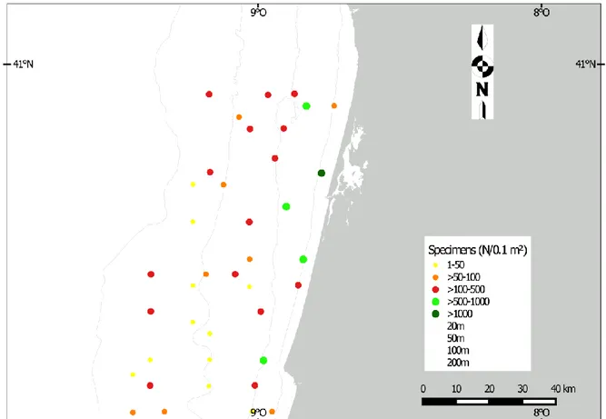
A total of 9532 specimens belonging to 197 species and 41 families were found (Annex 7.1). In all 39 sites polychaetes abundance per site ranged from 14 to 2584 specimens. The sites with a major number of polychaetes were the shallower, with 5 sites that reached or exceeded1000 individuals.The majority of sites (15) had a total abundance comprised between 100 and 500, followed by a total of 10 sites with specimens comprised between 50 and 100, and 9 sites with a range of 1 and 50 specimens (fig.3.1a).

16

The families with the highest number of species were Syllidae with 18 species, Spionidae with 17, Cirratulidae with 13, Paraonidae with 10 and Ampharetidae, Lumbrineridae, Maldanidae and Phyllodocidae with a total of 9 species.

The most abundant families were Phyllodocidae (3616 ind.), Capitellidae (1071 ind.), Sigalionidae (859 ind.), Syllidae (635 ind.) and Dorvilleidae (506 ind.). The 5 species with the highest abundance were Hesionura elongata (family Phyllodocidae; 36.8% of the total abundance, Aт), Mediomastus fragilis (family Capitellidae; Aт =10.5%), Pisione parapari (family Sigalionidae; Aт=7%), Protodorvillea kefersteini (family Dorvilleidae; Aт=5.2%) and Polygordius appendiculatus (family Polygordiidae; Aт=4.9%).

The highest abundance value was of 2584 individuals per 0.1 m‾² in medium sand, followed by 885 and 824 individuals per 0.1 m‾², respectively in medium and fine sand. The lowest values were 20, 19 and 14 specimens per 0.1 m‾², found respectively in very coarse sand, fine gravel and mud.

Species richness highest values were 45 per 0.1 m‾², in medium sand, followed by 44 and 41 per 0.1 m‾² in fine gravel; the lowest values were 11, 10 and 8 per 0.1 m‾², in very coarse sand, fine sand and mud. The highest values of the diversity indices were: Margalef (d) 7.88, 7.80, 7.79 in coarse, very fine and fine sand; Pielou (J’) 0.97, 0.96, 0.95 in very fine, fine sand and fine gravel, respectively; Shannon-Wiener (H’) with 3.38, 3.34, 1.99 in very fine, fine and coarse sand; and Simpson with 0.972, 0.971, 0.968 in fine and very fine sand. The lowest ones were: Margalef with 2.05, 1.78, 1.65 in fine and medium sand, Pielou with 0.37, 0.30, 0.27 in coarse and medium sand, Shannon with 1.12, 0.78, 0.72 in coarse and medium sand, and Simpson with 0.386, 0.380, 0.352 in coarse and medium sand. The results of the diversity indices, showed, in general, that sites at depths shallower than 60 m presented lowest values. Of this range of bathymetry, a total of 13 sampled sites were analysed, of which 7 characterised by coarse sediments (fine gravel, very coarse sand, coarse sand), and 6 by medium and fine sands. The homogeneity of species abundance per each sampled site seemed to increase with

17

depth, according to the values of the Pielou index. This trend was less evident with the Margalef index (d), in which only few shallow sites reached high d values (tab. 3.1).

Sampling site S N d J' H'(loge) 1-Lambda' 9 A 16 93 3.3093592 0.7500965 2.0797091 0.8300608 9 B 12 19 3.735856 0.9572272 2.3786202 0.9473684 9 E 29 87 6.2697215 0.8002936 2.6948253 0.8770382 9 F 29 57 6.9254625 0.851872 2.8685051 0.9154135 10 A 30 211 5.4186788 0.8176375 2.7809466 0.891582 10 C 8 14 2.6524623 0.8881659 1.8468891 0.8681319 10 E 37 101 7.8004464 0.9361804 3.3804704 0.9687129 11 F 22 41 5.6549327 0.9354273 2.8914456 0.954878 12 A 39 885 5.6001045 0.41727 1.5286943 0.531076 12 C 30 50 7.4130443 0.9304331 3.1645865 0.962449 12 E 28 50 6.9017999 0.9249099 3.0819889 0.957551 13 D 24 45 6.0420382 0.9699042 3.0824076 0.9717172 14 D 23 39 6.0050852 0.9585771 3.005613 0.9689609 15 B 28 141 5.4030124 0.6838597 2.2787605 0.7906784 15 F 39 124 7.8833569 0.8733872 3.1997079 0.9454498 16 A 15 119 2.9294075 0.6381464 1.7281325 0.6877938 16 C 11 20 3.338082 0.8986144 2.1547832 0.8947368 16 E 12 19 3.735856 0.9389474 2.3331967 0.9356725 17 C 32 277 5.5120739 0.7461007 2.585788 0.8833778 17 D 34 91 7.315679 0.8912848 3.1429914 0.9492063 17 F 45 304 7.6963069 0.57859 2.2024967 0.6781093 18 A 13 824 1.7872647 0.3070856 0.7876591 0.3527292 18 C 23 58 5.418128 0.8744191 2.7417359 0.922565 20 C 31 166 5.8685586 0.8477706 2.9112335 0.9264695 20 E 22 37 5.8156958 0.9484005 2.9315463 0.963964 21 A 24 750 3.4742818 0.5699897 1.8114581 0.7731126 22 D 18 73 3.9622796 0.6613621 1.9115823 0.7317352 22 E 21 30 5.8802821 0.9531573 2.9019087 0.9655172 23 A 14 2584 1.6545558 0.272233 0.7184386 0.3860488 23 E 20 113 4.0191329 0.3743621 1.1214887 0.3800569 24 B 41 329 6.9012425 0.8080459 3.0007367 0.9172289 25 C 33 194 6.0745751 0.8390978 2.9339117 0.9286897 25 D 29 150 5.5881138 0.7727975 2.6022379 0.8605817 26 D 34 69 7.7938521 0.9467797 3.3386866 0.9710145 27 A 10 79 2.0597568 0.5242724 1.2071817 0.5186628 27 B 25 575 3.7769283 0.4323344 1.3916306 0.4990456 28 B 44 450 7.03851 0.600982 2.2742297 0.7421727 28 C 25 155 4.7586708 0.7569972 2.43668 0.8329284 28 E 34 109 7.0342257 0.8372679 2.9525085 0.9245668

Table 3.1 Diversity indices. S= no. species; N= no. specimens;d= Margalef index; J’= Pielou eveness index; H’= Shannon-Wiener diversity index; 1- λ’= Simpson diversity index. In red the highest values, in yellow the lowest ones.

18

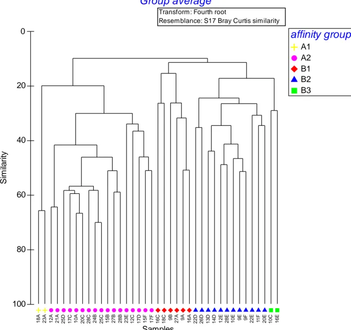
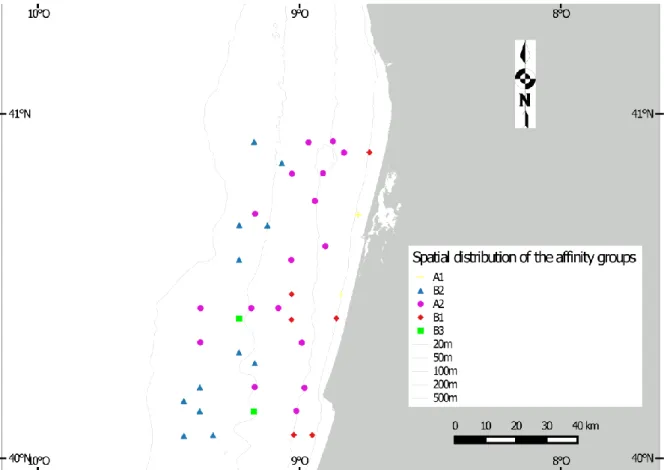
The results of the cluster analysis based on the abundance data are shown in the figure 3.1b. Following the first ramification at 15% of similarity, two affinity groups appeared (group A and B). The group A is divided, with a similarity of 20% in two groups, A1 and A2; the group B gathered B1, B2 and B3 with a similarity of 20 % and 30%. In the figure 3.1cis plotted the distribution of the groups. Almost all the sites of the group B2 and B3 occurred between the isobaths of 100 and 200 meters of depth; the group B1 didn’t exceed 70 m of depth. The sites in the group A1 were both along the isobath of 20 m and sites in the group A2 were all, except for three sites, lower than 100 m of depth.

Group average

Transform: Fourth root

Resemblance: S17 Bray Curtis similarity

affinity group

Figure 3.1b Cluster analysis based on the abundance of polychaetes. Subdivision in biological affinity groups based on different resemblance levels.

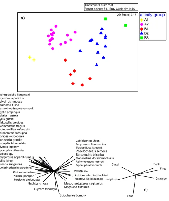
19 Figure 3.1d a showed the nMDS with the affinity groups plotted. Polychaete species found in

the study area, in the figure 3.1d b, are superimposed on the analysis to explain distribution of each site in the plot. It is possible to see the sites in the left side of the plot, in which were distributed the groups A1 and A2, is explained by various species, of which some are exclusive of both groups, e.g. Oxydromus pallidus, Psamathe fusca, Eulalia mustela (tab. 3.1a). In the right side of the plot, clearly, the species Labioleanira yhleni, Ampharete finmarchica and Poecilochaetus serpens described the group B3. Further, this species are also exclusive of this group (tab 3.1a); various species, e.g. Terebellides stroemii, Sarsonuphis bihanica, Aricidea (Aricidea) laubieri, described the group B2. Again, some of the species are characteristic or exclusive. The group B1 is supported by Glycera tridactyla and Spiophanes bombyx. The environmental data used as vectors (fig 3.1d c) showed that grain size (median), depth and fine

20

contents seemed to describe the deeper groups (B2 and B3), instead longitude, gravel and sand fractions described both groups A, and B1.

Table 3.1apresents the overall characteristics of the various affinity groups.

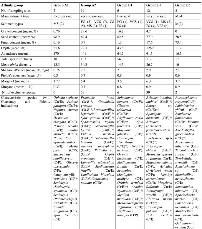
The group A1 comprised 2 sites and was characterised only by medium sand. It is the shallowest group, with the highest value of sand fraction. These groups showed the highest abundance and the lowest values the diversity indices. No exclusive were species found, and the most characteristic were Ophelia neglecta, Pisione parapari, Nephtys cirrosa and Hesionura elongata.

The group A2 comprised 17 sites and was characterised by a prevalence of coarser sediments; sand fraction was the most abundant, followed by gravel. Fine sediments were low. This assemblage reached the highest value of species richness. In this group was also recorded the highest abundance of syllids (7.41%). In this group a total of 59 exclusive species were recorded, and the most characteristic were Psamathe fusca, Goniadella gracilis, Protodorvillea kefersteini and Syllis garciai.

The group B1 included 6 sites of sand sediments. The most abundant sediment fraction was sand, followed by gravels and a low percentage of fine sediments. Abundance, species richness and diversity indices were moderate comparing with the other groups. The exclusive species were 6 and the most characteristic were S. bombyx, G. tridactyla, Phyllodoce rosea and Spio filicornis.

The group B2 included 12 sites and was characterised by a prevalence of sand. Abundance of the sandy fraction, was followed by the contents of fine sand and gravel. It was the deepest group with high values of abundance, species richness and diversity. Paraonidae family in this group reached also the highest abundance (10.98%). The exclusive species were 39 and the most characteristic species A. laubieri, Amage sp., Aponuphis brementi and A. pseudoarticulata.

21

The group B3 gathered only 2 sites, characterised by mud sediments. Sediment in these sites lacked gravel, sandy fraction was low and the highest level of fine contents was recorded. Only two exclusive species were found, and the most characteristic were P. serpens, L. yhleni, A. finmarchica and Melinna sp.1.

Affinity group Group A1 Group A2 Group B1 Group B2 Group B3

Nr. of sampling sites 2 19 6 12 2

Main sediment type medium sand very coarse sand fine sand very fine sand Mud Sediment types MS (2) FG (3), VCS (7), CS _{(5), MS (3), FS (1)} FG (1), VCS (1), _{FS (4)} VCS (1), MS (2), _{FS (3), VFS (6)} M(2)

Gravel content (mean; %) 0.76 29.6 16.2 4.7 0

Sand content (mean; %) 98.9 69.4 82.5 77.9 26.8

Fines content (mean; %) 0.16 0.9 1.3 17.6 73.4

Depth (mean; m) 21.6 72.3 43.8 126.8 113.6

Abundance (mean) 1704 441 64.7 61.5 16.5

Total species richness 18 137 56 112 17

Mean alpha diversity 13.5 30.3 14.5 26.7 10

Shannon-Wiener (mean; H', logn) 0.75 2.3 2 2.9 2.1

Pielou's evenness (mean; J') 0.3 0.7 0.8 0.9 0.9

Margalef (mean; d) 1.72 5.4 3.5 6.3 3.2

Simpson (mean; 1- λ') 0.37 0.7 0.8 0.9 0.9

Nr. of exclusive species 0 59 6 39 2

Characteristic species (with Constancy and Fidelity indications) Ophelia neglecta (Cn/E); Pisione parapari (Cn/P); Nepthys cirrosa (Cn/I); Hesionura elongata (Cn/I); Pisione remota (Cn/I); Eulalia mustela (Cn/I); Polygordius appendiculatus (Cn/I); Mysta picta (C/P); Saccocirrus papillocercus (C/P); Glycera oxycephala ( C/P); Parapionosyllis brevicirra (C/P); Scolelepis (Scolelepis) squamata (C/I); Scolelepis (Parascolelepis) tridentata (C/I); Eumida sanguinea (C/I); Spio decoratus (C/I) Psamathe fusca (Cn/E)*; Goniadella gracilis (Cn/E)*;Protodorvillea kefersteini (Cn/E)*;

Syllis garciai (Cn/E)*;

Sphaerosyllis taylori (Cn/P); Sphaerosyllis hystrix (Cn(E)*; Eulalia mustela (Cn/E)*; Sphaerosyllis bulbosa (Cn/P); Aonides oxycephala (Cn/P); Pulliella sp. (C/E)*; Gyptis propinqua (C/E)*; Eurysyllis tuberculata (C/E)*; Mediomastus fragilis (Cn/I); Caulleriella bioculata (C/E)*;Oxydromus pallidus (C/E)* Spiophanes bombyx (Cn/P); Glycera tridactyla (Cn/E)*; Phyllodoce rosea (C/E)*; Spio filicornis (C/P); Magelona johnstoni (C/P); Prionospio steenstrupi (C/E)*; Nepthys assimilis (C/P); Owenia fusiformis (C/I); Mediomastus fragilis (Cn/I); Scoloplos (Scoloplos) armiger (C/I); Orbinia sertulata (O/E)*; Acholoe squamosa (O/E)*; Sigalion mathildae (O/E)*; Mesochaetopterus sagittarius (C/I); Phyllodoce longipes (O/P) Aricidea (Acmira) laubieri (Cn/E)*; Amage sp. (Cn/E)*; Aponuphis brementi (C/E)*; Aricidea (Aricidea) pseudoarticulata (Cn/P); Euclymene sp.A (C/E)*; Prionospio ehlersi (C/E)*; Mesochaetopterus sagittarius (Cn/I); Magelona minuta (C/P); Aricidea (Aricidea) wassi (C/P); Nepthys kersivalensis (Cn/I); Magelona filiformis (Cn/I); Pterolysippe vanelli (C/E)*; Chirimia biceps (C/E)*; Prionospio pulchra (C/E)*; Pista cristata (C/I) Poecilochaetus serpens(Cn/P); Labioleanira yhleni (Cn/P); Ampharete finmarchica (Cn/I)*; Melinna sp.1 (C/E)*; Ancilostryllis groenlandica (C/E)*; Abyssoninoe hibernica (C/P); Trichobranchus roseus (C/P); Terebellides stroemii (C/I); Aphelochaeta sp. (C/I); Monticellina heterochaeta (C/I); Sarsonuphis bihanica (C/I); Aphelochaeta marioni (C/I); Lumbrineris lusitanica (C/I); Monticellina dorsobranchialis (C/I); Galathowenia oculata (C/I)

Table 3.1a Total characterisation of each affinity group. FG= fine gravel; VCS= very coarse sand; CS= coarse sand; MS= medium sand; FS= fine sand; VFS= very fine sand; M= mud. Constancy: Cn = constant, C = common, O = occasional; Fidelity: E = elective, P = preferential, I = indifferent; * = exclusive species in each group

22

Except done for the group A1, the diversity indices highlighted a good homogeneity in specie abundance per each group (tab. 3.1a). A1, on the contrary, showed the highest value of abundance, but low values of d, H’, J’ and 1- λ'.

The analyses of the relationships between the environmental variables and the structure of the polychate assemblages, done with BIOENV routine, showed that depth, grain size (median) and fine contents were the best related with the biological data (rho=0.598, significance of 0.1%).

23

Transform : Fourth root

Resem blance: S17 Bray Curtis sim ilarity

affinity group A1 A2 B1 B2 B3 2D Stress: 0.15 Labioleanira yhleni Ampharete finmarchica Terebellides stroemii Poecilochaetus serpens Sarsonuphis bihanica Monticellina dorsobranchialis Aphelochaeta marioni Aponuphis brementi Amage sp.

Aricidea (Acmira) laubieri Nephtys kersivalensis Mesochaetopterus sagittarius Magelona filiformis Glycera tridactyla Spiophanes bombyx Nephtys cirrosa Hesionura elongata Pisione remota Pisione parapari Malmgreniella ljungmani Oxydromus pallidus Polycirrus medusa Psamathe fusca Harmothoe fraserthomsoni Gyptis propinqua Eulalia mustela Syllis garciai Plakosyllis brevipes Mediomastus fragilis Protodorvillea kefersteini Paraehlersia ferrugina Aonides oxycephala Goniadella gracilis Eurysyllis tuberculata Glycera lapidum Aponuphis bilineata Pulliella sp. Polygordius appendiculatus Syllis licheri Eumida sanguinea Lumbrineriopsis paradoxa Gravel Longitude Sand Depth Fines Grain size

Figure 3.1d a) nMDS based on the abundance of polychaetes; b) polychaete species as vectors with Spearman correlation (rho>0.5); c) environmental data used as vectors with Spearman correlation (rho>0.5).

a)

24 3.2- Description of selected families

Following WoRMS website (Read, 2015) scheme, a classic, commonly accepted way to classify polychaete families is into Errantia and Sedentaria subclasses. A brief description of some selected families is presented in this section, based on DELTA database (Dallwitz et al., 2010), on the interactive key Polikey (Glasby & Fauchald, 2003), and on the book Polychaetes (Rouse & Pleijel, 2001), together with a commenting on their distribution in the study area.

SUBCLASS: SEDENTARIA Infraclass: Scolecida

Family: Capitellidae

Family authority: Grube, 1862.

Capitellids are marine, freshwater or estuarine deposit feeders, present from the coastal shelf to the deep sea and distributed worldwide.

Their body is vermiform in shape, characterised by a division in thorax (with capillary chaetae only) and abdomen (with long-handled hooks) (plate I c-d, annex 2); the head has no appendages and appears discrete and compact. Pygidium is simple ring or cone, or plate-like (rarely). Pygidial appendages absent, or present; one pair of cirri, or single medial cirrus. Branchiae, if present, may be retractile and arise from the parapodia or from the dorsum. Their range size is from less than 10 mm to more than 200 mm.

Capitellids live in mucus-lined burrow or tubes, in detritus, mud and fine sand/mud sediments. Some species of the Capitella capitata complex are used as indicators of organic pollution because of their spread in areas with reduced species diversity due to natural causes or anthropogenic effects.

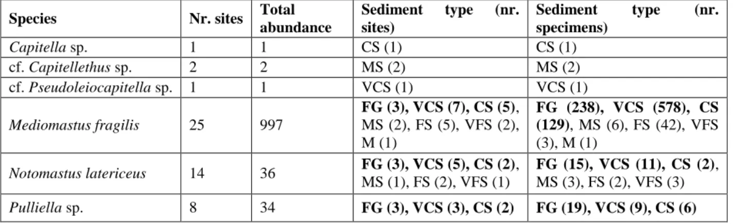
25 3.2a showed that the most abundant species were Mediomastus fragilis Rasmussen, 1973, Notomastus latericeus Sars, 1851 and Pulliella sp. Gravier, 1904. In general these species occurred more and with a higher abundance in coarse sediments; M. fragilis and N. latericeus were found in all the sediment types, even if with clearly different abundances. Further, M. fragilis is a characteristic species of the group A2 sites, and Pulliella sp. is exclusive of it (tab. 3.1a).

The distribution of the abundance of the Capitellids may be appreciate in figure 3.2a, in which it is possible to see how M. fragilis distribution covered almost all the study area, but the abundance was higher in shallow water. N. latericeus and Pulliella sp. showed distributions concentrated mainly in the N-NE part of the study area, characterised by coarse sediments.

Table 3.2a Capitellids with the number of sites in which they were found, the total abundance of the species, the number of sites per sediment type, and the abundance of each species per sediment type. FG= fine gravel; VCS= very coarse sand; CS= coarse sand; MS= medium sand; FS= fine sand; VFS= very fine sand; M= mud. In bold the sediment types in which species were more abundant.

Species Nr. sites Total abundance Sediment type (nr. sites) Sediment type (nr. specimens) Capitella sp. 1 1 CS (1) CS (1) cf. Capitellethus sp. 2 2 MS (2) MS (2) cf. Pseudoleiocapitella sp. 1 1 VCS (1) VCS (1) Mediomastus fragilis 25 997 FG (3), VCS (7), CS (5), MS (2), FS (5), VFS (2), M (1) FG (238), VCS (578), CS (129), MS (6), FS (42), VFS (3), M (1) Notomastus latericeus 14 36 FG (3), VCS (5), CS (2), MS (1), FS (2), VFS (1) FG (15), VCS (11), CS (2), MS (3), FS (2), VFS (3) Pulliella sp. 8 34 FG (3), VCS (3), CS (2) FG (19), VCS (9), CS (6)

26

a) b)

c)

27 Order: Spionida

Suborder: Spioniformia Family: Spionidae

Family authority: Grube, 1850

Spionids are marine worms present from the shallow water to the deep sea. Their distribution is worldwide.

These animals have a vermiform body-shape with numerous segments (more than about 15). Head is discrete and compact; prostomium shape is triangular to trapezoidal (narrow end posteriorly), or T-shaped. Prostomial antennae present, or absent. Grooved palps paired, dorsolateral. Pygidium- simple ring or cone, or with multiple digitate lobes; pygidial appendages present. Branchiae present, arising from the parapodia or from the dorsum. Range size goes from several mm to several cm (plate III a-b, annex 2).

Spionids are deposit or filter feeders; they may occur on soft or hard substrata; some species are epizoic (on mollusc shells). Tubes, if present, membranous.

This family includes 282 specimens belonging to 17 species. Spionids were distributed over the whole study area, occurring in 35/39 sites and in all sediment types, except mud (tab. 3.2b; fig.

3.2b a).

The most abundant species were Prionospio multibranchiata Berkeley, 1927, Spiophanes bombyx (Claparède, 1870) and Aonides oxycephala (Sars, 1862). P. multibranchiata was found with a total of 64 specimens in 18 sites. This species occurred from fine gravel to very fine sand; the abundance was higher in medium-fine sediments (medium sand, fine sand, very fine sand). S. bombyx was found with a total of 52 specimens in 13 sites. Fine and very fine sand were the sediment types in which the species occurred more often with a total of 8/13 sites. Also the abundance was higher in these sediments with a total of 39/52 specimens. A. oxycephala was found with a total of 48 specimens distributed in 16 sites with the following

28

sediment types: fine gravel, very coarse sand, coarse sand, medium sand and fine sand. Further, A. oxycephala is a characteristic species of the group A2, and S. bombyx of the group B1 (tab. 3.1a). In the figure 3.2b b is possible to see that almost all the sites were located at depth less

than 100 m. This species seemed to be more abundant in coarser sediments (fine gravel, very coarse and coarse sand) with a total of 40/48 animals.

Table 3.2b Spionids with the number of sites in which they were found, the total abundance of the species, the number of sites per sediment type, and the abundance of each species per sediment type. FG= fine gravel; VCS= very coarse sand; CS= fine sand; MS= medium sand; FS= fine sand; VFS= very fine sand. In bold the sediment types in which species were more abundant.

Species Nr. sites Total

abundance Sediment type (nr. sites)

Sediment type (nr. specimens) Aonides oxycephala 16 48 FG (3), VCS (7), CS (3), MS (1), FS (2) FG (16), VCS (18), CS (6), MS (1), FS (7) Laonice bahusiensis 5 11 FG (1), VCS (1), CS (1), FS (1), VFS (1) FG (1), VCS (1), CS (1), FS (1), VFS (7) Paraprionospio pinnata 3 4 VFS (3) VFS (4) Prionospio aluta 1 1 VFS (1) VFS (1) Prionospio ehlersi 5 21 VCS (1), MS (1), FS (1), VFS (2) VCS (4), MS (9), FS (3), VFS (5) Prionospio fallax 3 3 VCS (1), FS (2) VCS (1), FS (2) Prionospio multibranchiata 18 64 FG (1), VCS (6), CS (3), MS (2), FS (3), VFS (3) FG (2), VCS (14), CS (14), MS (15), FS (16), VFS (3) Prionospio pulchra 4 7 FS (1), VFS (3) FS (2), VFS (5) Prionospio sp. 2 3 VCS (1), VFS (1) VCS (2), VFS (1) Prionospio steenstrupi 2 2 FG (1), FS (1) FG (1), FS (1) Scolelepis (Parascolelepis) tridentate 5 17 CS (1), MS (1), FS (3) CS (1), MS (3), FS (13) Scolelepis (Scolelepis) squamata 4 8 VCS (1), MS (1), FS (2) VCS (1), MS (1), FS (6) Scolelepis sp. 1 1 FS (1) FS (1) Spio decoratus 9 21 VCS (2), CS (2), MS (1), FS (3) VCS (9), CS (7), MS (1), FS (3) Spio filicornis 4 10 VCS (1), FS (3) VCS (6), FS (4) Spiophanes bombyx 13 52 FG (1), VCS (2), CS (1), MS (1), FS (7), VFS (1) FG (3), VCS (7), CS (2), MS (1), FS (38), VFS (1) Spiophanes kroyeri 5 9 CS (1), FS (2), VFS (2) CS (3), FS (3), VFS (3)

29 Figure 3.2b Abundance distribution of a) Spionidae family; b) Aonides oxycephala.

a)

30 Order: Terebellida

Suborder: Terebellomorpha Family: Terebellidae

Family authority: Johnston, 1846.

Terebellids (spaghetti worms) are marine worms, distributed worldwide, from the shallow water to the deep sea.

Spaghetti worms have a vermiform body-shape with or without division of the body in regions. The head bears many tentacles around the mouth. No palps. The pygidium is simple, in the shape of a cone or a ring, or with multiple lobes; no pygidial appendages. Branchiae, if present, occur from the dorsum, branching or filiform. Glandular ventral shield present. Range size is from 100 to 300 mm in length (plate III d-e, annex 2).

Terebellids are almost all deposit feeders, rarely may be filter feeders (using a mucus feeding net built into top of tube). Their tube, if present, is membranous, or leathery or parchment like. They may occur on soft substrata, or hard substrata (under stones and in crevices), or epizoic (algal holdfasts and seagrass).

A total of 121 Terebellids were found in the study area, belonging to 7 species plus 3 specimens of Terebellidae n.i. In general, almost all the species of this family occurred more in coarse sediments (fine gravel, very coarse sand, coarse sand) (tab. 3.2c). No species were found in mud. As is possible to see in the figure 3.2c, this family was well distributed in all the study area with a total of 27/39 sites. The most abundant species were Pista cristata (Müller, 1776) and Polycirrus medusa Grube, 1850. P. cristata was found with a total of 67 specimens, of which the most abundant were in coarse sediments (fine gravel, very coarse sand, coarse sand) with a total of 53/67 animals. This species is also characteristic of the group B2 (tab.

3.1a). P. medusa was found with a total of 37 specimens; of which 31/37 in coarse sediments

31 Table 3.2c Terebellids with the number of sites in which they were found, the total abundance of the species, the number of sites per sediment type, and the abundance of each species per sediment type. FG= fine gravel; VCS= very coarse sand; CS= coarse sand; MS= medium sand; FS= fine sand; VFS= very fine sand. In bold the sediment types in which species were more abundant.

Species Nr. sites Total

abundance Sediment type (nr. sites)

Sediment type (nr. specimens) Eupolymnia nebulosa 1 1 VFS (1) VFS (1) Lanice conchilega 5 9 VCS (1), CS (1), MS (1), VFS (2) VCS (1), CS (1), MS (4), VFS (3) Pista cristata 16 67 FG (2), VCS (7), CS (1), MS (2), FS (2), VFS (2) FG (5), VCS (47), CS (1), MS (4), FS (7), VFS (3) Pista lornensis 1 2 VCS (1) VCS (2) Polycirrus medusa 15 37 FG (4), VCS (5), CS (3), VFS (3) FG (14), VCS (8), CS (9), VFS (6) Streblosoma bairdi 1 1 MS (1) MS (1) Terebellidae n.i. 2 3 FG (1), MS (1) FG (1), MS (2) Neoamphitrite figulus 3 4 VCS (1), CS (1), MS (1) VCS (2), CS (1), MS (1)

32 SUBCLASS: ERRANTIA

Order: Phyllodocida Suborder: Aphroditiformia Family: Sigalionidae

Family authority: Malmgren, 1867.

Sigalionids (scaleworms) are marine worms present from the shallow water to the deep sea. They are cosmopolitan.

These animals have a vermiform body-shape with numerous segments (more than about 15). Head discrete and compact, with a rounded to oval (anteriorly truncate) prostomium. Two pairs of eyes, if present; prostomial antennae present, a pair anterolateral and a single medial one. Palps present. Pygidium simple with appendages. Branchiae present, digitiform, arising from the parapodia. Dorsal cirri modified as elytra (plate VI a-b, annex 2).

Sigalionids are raptorial feeders living in soft substrata.

Sigalionids were found with a total of 859 specimens belonging to 6 species. This family occurred in all the sediment types (tab. 3.2d), and, as the figure 3.2d a shows, the highest abundances were found in sites located up to 100 meters depth. The most abundant species were Pisione parapari Moreira, Quintas & Troncoso, 2000 and P. remota (Southern, 1914). P. parapari was found with a total of 670 specimens, reaching the peak of the abundance in medium-fine sediments (medium sand, fine sand). P. remota is characteristic of the group A1 (tab. 3.1a). It is possible to appreciate in the figure 3.2d b that all the animals were found between 20 and 50 m. P. remota was found with 167 specimens, of which 114 in medium and fine sand.

33 Table 3.2d Sigalionids with the number of sites in which they were found, the total abundance of the species, the number of sites per sediment type, and the abundance of each species per sediment type. FG= fine gravel; VCS= very coarse sand; CS= coarse sand; MS= medium sand; FS=fine sand; VFS= very fine sand; M= mud. In bold the sediment types in which species were more abundant.

Species Nr. sites Total

abundance Sediment type (nr. sites) Sediment type (nr. specimens)

Labioleanira yhleni 6 12 FS (1), VFS (3), M (2) FS (2, VFS (4), M (6) Pisione guanche 1 1 FG (1) FG (1) Pisione parapari 7 670 FG (2), VCS (1), CS (1), MS (2), FS (1) FG (3), VCS (6), CS (26), MS (610), FS (25) Pisione remota 13 167 FG (2), VCS (3), CS (4), MS (3), FS (1) FG (10), VCS (32), CS (11), MS (108), FS (6) Sigalion mathildae 1 3 FS (1) FS (3) Sthenelais limicola 3 6 FG (1), CS (1), MS (1) FG (2), CS (2), MS (2)

34 Figure 3.2d Abundance distribution of a) Sigalionidae family; b) Pisione parapari.

b) a)

35 Suborder: Nereidiformia

Family: Syllidae

Family authority: Grube, 1850.

Syllids are marine worms, present from the coastal shelf to the deep sea. Their distribution is worldwide.

These animals have a vermiform or grube-like body, dorsoventrally flattened. Head is discrete to compact; prostomium is rounded to oval (anteriorly truncate). Eyes present (two or three pairs) with or without compound lenses. Prostomial antennae present; palps paired, ventrolateral. Pygidium is simple with appendages. Branchiae absent. Proventricle with radiating muscle fibres. Range size is from around 1 mm to several cm (plate VI d-e, annex 2). Syllids may be raptorial feeders, or parasitic, or commensal living in both soft or hard substrata, or epizoic.

This family was found with a total of 635 specimens belonging to 18 species. Syllids occurred in 21/39 sites and the highest abundances, in general, were recorded in coarse sediments (fine gravel, very coarse sand, coarse sand). No individuals were found in very fine sand and mud. The figure 3.2e shows that almost all the sites (17/21) were located at depth less than 100 m. The most abundant species were Syllis garciai (Campoy, 1982) and Sphaerosyllis bulbosa Southern, 1914, both characteristic species of the group A2 (tab. 3.1a). S. garciai was found with a total of 207 specimens in 11/21 sites. This species reached the highest abundances in coarse sand. S. bulbosa was found with 170 animals in 14/21 sites, of which 11 were coarse sediments (fine gravel, very coarse sand, coarse sand). Also the highest abundances were found in these sediment types (tab. 3.2e).

36 Table 3.2e Syllids with the number of sites in which they were found, the total abundance of the species, the number of sites per sediment type, and the abundance of each species per sediment type. FG= fine gravel; VCS= very coarse sand; CS= coarse sand; MS= medium sand; FS=fine sand. In bold the sediment types in which species were more abundant.

Species Nr. sites Total

abundance Sediment type (nr. sites) Sediment type (nr. specimens) Eurysyllis tuberculate 8 70 FG (2), VCS (5), FS (1) FG (53), VCS (15), FS (2) Myrianida brachycephala 1 1 MS (1) MS (1) Paraehlersia ferrugina 5 9 FG (3), VCS (2) FG (6), VCS (3) Parapionosyllis brevicirra 2 7 VCS (1), MS (1) VCS (1), MS (6) Plakosyllis brevipes 5 10 FG (1), VCS (4) FG (1), VCS (9) Prosphaerosyllis campoyi 1 1 VCS (1) VCS (1) Salvatoria sp. 1 1 FG (1) FG (1) Sphaerosyllis bulbosa 14 170 FG (3), VCS (6), CS (2), MS (1), FS (2) FG (35), VCS (106), CS (23), MS (3), FS (3) Sphaerosyllis hystrix 10 16 FG (1), VCS (7), MS (1), FS (1) FG (1), VCS (12), MS (1), FS (2) Sphaerosyllis sp. 4 7 FG (2), VCS (1), MS (1) FG (5), VCS (1), MS (1) Sphaerosyllis taylori 13 53 FG (3), VCS (4), CS (3), MS (1), FS (2) FG (8), VCS (31), CS (7), MS (4), FS (3) Streptodonta pterochaeta 6 18 FG (2), VCS (2), CS (1), FS (1) FG (9), VCS (3), CS (5), FS (1) Streptosyllis bidentate 3 3 VCS (1),MS (1), FS (1) VCS (1),MS (1), FS (1) Syllides convolutes 2 3 CS (1), FS (1) CS (1), FS (2) Syllis garciai 11 207 FG (3), VCS (5), CS (3) FG (11), VCS (23), CS (173) Syllis licheri 9 40 FG (2), VCS (4), CS (1), FS (2) FG (9), VCS (16), CS (1), FS (14) Synmerosyllis lamelligera 4 17 FG (3), VCS (1) FG (16), VCS (1) Trypanosyllis (Trypanosyllis) coeliaca 1 2 FG (1) FG (2)

37 Subclass: Polychaeta incertae sedis

Family: Polygordiidae

Family authority: Czerniavsky, 1881

Polygordiids are marine worms of the continental shelf. Their distribution is cosmopolitan. Their body-shape is vermiform with a weak, or absent, segmentation. Head discrete and compact with a blunty conical to trapezoidal (narrow end anteriorly). Prostomial antennae present, paired arising anterolaterally. No palps. Pygidium simple ring or cone, or with multiple digitate lobes. Branchiae absent. No parapodia. Range size from 10 to 100 mm (plate VII a,

annex 2).

Polygordiids are interstitial worms living in soft substrata.

This family was found in the study area in 18 sites, with a total of 473 specimens belonging to the species Polygordius appendiculatus Fraipont, 1887. Polygordiids were sampled in 14 sites of coarser sediments (fine gravel, very coarse sand, coarse sand), 2 of medium sand and 2 of fine sediments (fine and very fine sand). No species were found in mud. The majority of the sites were shallower than 100 meters depth, reaching the highest abundances in the NE part of

38

the study area (fig. 3.2f). P. appendiculatus was also one of the characteristic specie of the group A1 (tab. 3.1a).

39

4 - DISCUSSION AND CONCLUSION

The aim of this section is to integrate and discuss all the results presented in the thesis.

Being the West Iberian Coast scarcely and recently studied, the aim of this work was focused on a more detailed description of the spatial distribution of the polychaete fauna in the Northwestern Portuguese Coastal Shelf. Polychaetes are one of the most abundant benthic taxa along the Portuguese Continental Shelf (Martins et al., 2013); in fact, despite the small area investigated, 197 species belonging to 41 families were found. In general, sediment characteristic, depth, salinity and temperature (Gray, 1974; Hutchings, 1998), as well as hydrodynamics, are the principal factor related to the distribution of this taxon (Simboura et al., 2000).

The species richness recorded in the study area may reflects the structure of the communities, characterised not only by small-sized fast-colonising species with high growth rates, but also by larger slowly growing species (Lourido et al., 2008). Moreover, the presence of families with different ecology and behaviour can be justified by the various types of the sediments that characterise this part of the Portuguese Coastal Shelf, ranging from fine gravel to mud. Such sediment diversity was attributed by Martins et al., (2012) to the co-existence of a number of driving factors, namely mainland lithology, fluvial input, hydrodynamics, physiography of the shelf (slope, morphological barriers), but also the biological activity, paleoclimatic changes and anthropogenic contamination. The precipitation and the presence of rivers play also an important role in the large fluvial input in this sector of the shelf. In general, the northwestern sector is characterised by a discontinuous seaward decreasing trend in grain size, because of the presence of some relict deposits (Abrantes & Rocha, 2007). According to this scenario, the results of BIOENV routine could be interpreted, giving importance to these variables and to their correlation with the polychaete assemblages.

40

The decreasing abundance trend related to the depth confirms what Martins et al., (2013) described for the Portuguese shelf and also agrees to what other authors reported for different coasts around the world, e.g. Brooks et al., (2006); Moulaert et al., (2007), Montiel et al., (2011), Hernández-Alcántara et al., (2014). Obviously, as Fitzhugh, (1984) wrote, polychaete distribution was not only influenced by the depth itself, but also by other depth-related parameters, as bottom-water variability, sedimentary stability and food availability. In this work, maybe for the small-scale observation, latitude did not seem to influence the patterns of distribution.

In this study, for the first time, mud assemblages were recorded and described in the Northwestern part of the Shelf. The presence of this group (B3) at depth higher than 100m, and the low number of sites belonging to it, may be explained by the extremely energetic regime of waves and tides characterising in this sector, that remove and deplete the fine component of the sediments. This affinity group was characterised by the species Labioleanira yhleni, Poecilochaetus serpens and Ampharete finmarchica. All these species occur in soft substrata, and in particular P. serpens and A. finmarchica are both tubiculous deposit or filter feeders. Furthermore, L. yhleni is known already in the literature to be representative of silt assemblages in other parts of the world (e.g. Papazacharias & Voultsiadou, 1998; Simboura et al., 2000), and it is an important bioturbator of soft substrata (Queirós et al., 2013). It is also important to underline how, despite having low values of the diversity indices, the group B3che gruppo B3? and its sediment composition played a role in the general trend of the polychaete distribution as revealed in BIOENV routine.

The groups with the highest mixture in sediment types (groups A2 and B2) reached the highest values in species richness and diversity indices and the exclusive species were all of relatively small sizes belonging to the families e.g. Dorvilleidae, Hesionidae, Spionidae, Paraonidae, Sigalionidae and Syllidae. This may be related to the heterogeneity established in these mixed sediments that provide interstitial spaces for small specimens of these families. Further, the

41

considerable abundance of the latter family may be explained also by their wide diversity of the reproductive phenomena (Franke, 1999).

Also the considerably high abundance of Capitellidae family may be explained in this study by their high reproductive capability, being characterised by opportunistic species inhabitant of polluted and disturbed areas (Papazacharias & Voultsiadou, 1998; Horng & Taghon, 1999; Stark et al., 2014). Polluted areas are related in literature to fine and silt sediments (e.g Palanques & Diaz, 1994; Ünlü & Alpar, 2015), on the contrary in this work these specimens reached the highest abundances in fine gravel, very coarse sand and coarse sand. Moreover, as Martins et al., (2012) said, the Portuguese Continental Shelf, except done for some located areas nearshore, seems to be non- polluted; it may be endorsed by the presence also of other families or species (e.g. Maldanidae, Lumbrineridae, Terebellidae, and Terebellides stroemii, Scalibregma inflatum) linked to the good state of the habitat (Dean, 2008). Further, the most abundant capitellid was Mediomastus fragilis, considered only tolerant to pollution, but not an indicator species.

On the other hand, the lowest values of biodiversity indices were reached in one of the groups with the highest homogeneity of sediment types (e.g. A1), confirming the data from literature about the lower faunal diversity related to the homogeneity of the sediment and the scarcity of microhabitats (Moreira et al., 2006). This group (A1), the medium sand one, did not show exclusive species and characteristic ones, e.g. P. parapari, P. remota and Hesionura elongata, whilst in previous studies these species were generally related to coarser assemblages (Byrnes et al. 2003; Martins et al., 2013).

Spiophanes bombyx, one of the characteristic species of the group B1, in literature, as well as in this study, is linked to fine sand assemblages with Glycera tridactyla (Moreira et al., 2010; NPWS, 2011; Martins et al., 2013) strengthening the correlation between these species and sand sediments. An exclusive species of this group was also Phyllodoce rosea, species present only in the Northwestern sector of the shelf (Martins, 2013).

42

The affinity among groups found in this work generally support the ones belonging to the northwestern sector described by Martins et al., (2013). Actually, except for the mud assemblages that are newly described for this sector, the coarser sediment assemblages (A1 and A2) presented the same characteristic species belonging to the Syllidae and Sigalionidae families, as well as the assemblages of fine and very fine sand (B1 and B2) were characterised by species of Terebellidae and Magelonidae.

In conclusion, this study allows to have a more complete view of the polychaete fauna in the Northwestern part of the Portuguese Continental Shelf. In fact, not only the general spatial distribution of polychaetes and the relationships found with the environmental parameters, as depth and grain size, endorsed previous studies done in different parts of the world, but, thanks to the high sampling effort, mud assemblages were firstly described and some species representative of coarser mixed assemblages (fine gravel, very coarse and coarse sand) occurred and appeared as characteristic of a sandy homogeneous groups. Future studies may be done to analyse and better understand which other parameters might influence the distribution of species (e.g. Phyllodoce rosea) or families not explained yet.

43

5- BIBLIOGRAPHY

Abrantes I, Rocha F. 2007. Sedimentary Dynamics of the Aveiro Shelf (Portugal). Journal of Coastal Research 1005–1009.

Aguirrezabalaga F, Gil J. 2009. Paraonidae (Polychaeta) from the Capbreton Canyon (Bay of Biscay, NE Atlantic) with the description of eight new species. Scientia Marina 73: 631– 666.

Alveirinho Dias JM, Nittrouer CA. 1984. Continental shelf sediments of northern Portugal. Continental Shelf Research 3: 147–165.

Banse K. 1969. Acrocirridae n.fam. (Polychaeta Sedentaria). J Fish Res Board Can 26: 2595– 2620.

Banse K. 1979. Sabellidae (Polychaeta) principally from the Northeast Pacific Ocean. Journal de l’Office des recherches sur les pecheries du Canada 36: .

Barnich R, Fiege D. 2003. The Aphroditoidea (Annelida: Polychaeta) of the Mediterranean Sea. Frankfurt: Abh. senckenberg. naturforsch. Ges.

Barwick K. 2006. Key to the Paraonidae ( Annelida : Polychaeta ) reported from the City of San Diego Ocean Monitoring program. 1: .

Bettencourt AM, Bricker SB, Ferreira JG, Franco A, Marques JC, Melo JJ, Nobre A, Ramos L, Reis CS, Salas F, Silva MC, Simas T, Wolff WJ. 2004. Typology and reference conditions for Portuguese transitional and coastal waters. INAG and IMAR.

Bhaud M, Lastra MC, Petersen ME. 1994. Redescription of Spiochaetopteus solitarius (Rioja, 1917), with notes on tube structure and comments on the generic status (Polychaeta: Chaetopteridae). Ophelia 40: 115–133.

Bick A, Otte K, Meißner K. 2010. A contribution to the taxonomy of spio (Spionidae, Polychaeta, Annelida) occurring in the north and baltic seas, with a key to species recorded in this area. Marine Biodiversity 40: 161–180.

Blake JA. 1996. Family Paraonidae, Cerruti, 1909. Blake, James A., Brigitte Hilbig & Paul H. Scott (eds.). Taxonomic Atlas of the Benthic Fauna of the Santa Maria Basin and the Western Santa Barbara Channel. Volume 6, The Annelida Part 3: Polychaeta: Orbiniidae to Cossuridae. Santa Barbara, California: Santa Barbara Museum of Natural History. p. 27–70.

Brito MC, Nunez J. 2002. A new genus and species of Questidae (Annelida: Polychaeta) from the central Macaronesian region and a cladistic analysis of the family. Sarsia: North Atlantic Marine Science 87: 281–289.

44

continental shelf: a literature synopsis of benthic faunal resources. Cont. Shelf Res. 26: 804–818.

Byrnes MR, Hammer, R.M, Vittor BA, Kelley SW, Snyder, D.B. Côté JM, Ramsey JS, Thibaut TD, Phillips, N.W. Wood JD, Germano JD. 2003. Collection of Environmental Data Within Sand Resource Areas Offshore North Carolina and the Environmental Implications of Sand Removal for Coastal and Beach Restoration. .

Cacabelos E, Moreira J, Troncoso JS. 2008. Distribution of Polychaeta in soft-bottoms of a Galician Ria (NW Spain). Scientia marina 72: 655–667.

Cantone G. 1989. Censimento dei policheti dei mari italiani Poecilochaetidae. Atti soc. Tosc. Sci. Nat. 23–29.

Capaccioni-Azzati R, Martin D. 1992. Pseudomastus deltaicus gen. et sp. n. (Polychaeta: Capitellidae ) from a shallow water bay in the North- Western Mediterranean Sea. Zoologica Scripta 21: 247–250.

Castelli A, Valentini A. 1995. Censimento dei policheti dei mari Italiani Pectinariidae. Atti soc. Tosc. Sci. Nat. Mem., Seri: 51–54.

Chambers S, Lanera P, Mikac B. 2011. Chaetozone carpenteri, McIntosh, 1911 from the Mediterranean Sea and records of other bi-tentaculate Cirratulids. 37–41.

Chambers SJ, Garwood PR. 1992. Polychaetes from Scottish waters. A guide to identification. Part 3. Family Nereidae. Scotland: National Museums of Scotland.

Clarke KR, Gorley RN. 2006. PRIMER v.6: User Manual/Tutorial PRIMER-E. 190.

Costa PFE, Gil J, Passos AM, Pereira P, Melo P, Batista F, da Fonseca LC. 2006. SCIENTIFIC ADVANCES IN POLYCHAETE The market features of imported non-indigenous

polychaetes in Portugal and consequent ecological concerns. Scientia Marina 70S3: 287– 292.

Dajoz R. 1971. Précis d’Ecologie. Paris: Ed. Dunod.

Dallwitz MJ, Paine TA, Zurcher EJ. 2010. User’s Guide to the DELTA Editor. Delta 1–31. Dean H. 2008. The use of polychaetes (Annelida) as indicator species of marine pollution: a

review. Rev Biol Trop 56: 11–38.

DeKluijver MJ, Ingalsuo SS, vanNieuwenhuijzen AJL, Veldhuijzen van Zanten HH. 2015. [Internet]. Available from:

http://species-identification.org/species.php?species_group=Macrobenthos_polychaeta&selected=foto& menuentry=inleiding&record=Introduction

Fauchald K. 1982. Revision of Onuphis, Nothria, and Paradiopatra (Polychaeta: Onuphidae) based upon type material. Smithsonian Contributions to Zoology 356: .

Fauchald K. 1992. A Review of the Genus Eunice (Polychaeta: Eunicidae) Based upon Type Material. Smithsonian Contributions to Zoology 1–422.