1
Università di Pisa
Facoltà di Ingegneria
Corso di Laurea Specialistica in Ingegneria Biomedica
Tecniche Elettrotomografiche per la
Caratterizzazione di Tessuti Biologici
Il candidato: Primo relatore:
Caltagirone Laura Menciassi Arianna
Secondo relatore:
Giardini Mario E.
2
University of St Andrews, Scotland.
This work has been carried out in collaboration with the School of Medicine of the University of St Andrews, Scotland, UK.
Supervisor:
Giardini Mario E.
3 The warrior of the light believes. Just like children believe. Because he believes in miracles, miracles begin to happen.
Because he is sure that his thought can change his life, his life begins to change. Because he is sure that he will find love, this love appears. From time to time he is disappointed. Sometimes he gets hurt. And then he hears comments like: "that fellow's so naive!" But the warrior knows that it is all worthwhile. For each defeat he counts two victories in his favor.
4
Acknowledgements
First and foremost I would like sincerely thank my advisor Mario Ettore Giardini for tactfully providing direction throughout my Thesis, for giving unique solutions in the laboratory, for helping hand throughout the entire project, for believing in my work and for giving an introduction to the world of research.
I would like also to express my gratitude to St. Andrews University in Scotland, and in particular the School of Medicine, for providing financial support and facilities. There I could find a very appropriate place to study. Thanks to Arianna Menciassi for directing me to the right people for preparing the Thesis. Then great tanks go to the Biophotonics team, for your humor and smiles. I wish to thank my parents for bringing me up in an environment that appreciated studies and research.
A special thanks is due to my friend Nicola Melville, who has celebrated with me my joy in success of these wonderful experience, and Franceschini Ferruccio for helping me in the translation of this Thesis and for you friendship.
Finally, enormous thanks to Marcoandrea for his support throughout my Master‟s study. Everything is easier and delightful with you. My life is completely changed with you and you are the reason for where and who I am.
5
Abstract
Electrical impedance tomography (EIT) is an imaging modality wherein the spatial map of conductivity and permittivity inside a medium is obtained from a set of surface electrical measurements. Electrodes are brought into contact with the surface of the object being imaged and a set of currents are applied and the corresponding voltages are measured. These voltages and currents are then used to estimate the electrical properties of the object using an image reconstruction algorithm which relies on an accurate model of the electrical interaction. The process of property estimation, called inverse problem, is highly nonlinear, ill-conditioned, and ill-posed. Reconstruction of the electrical properties distribution is an under-determined problem requiring a regularization method.
EIT has been researched extensively in the medical field, as well as in other technological areas, such as industrial process control, chemical engineering and geotechnical research. The technique has become an independent, fully-featured stream in the biomedical engineering field, and has high clinical potential as an investigation tool. The objective of this Thesis was to develop a device for EIT imaging, which could be convenient, noninvasive, easily programmable, portable and relatively inexpensive.
In this direction a simple EIT system and its hardware and software parts have been developed. Two 16-electrodes probes in circular and planar geometry were built for treating two and three-dimensional samples. Probes and a circuit board, comprehending a serial programmable interface and a switch based multiplexer, have been built and connected to a Lock-in amplifier, used as excitation source and acquisition system. As the object of EIT is a human body part, the current must be limited within the range regulated by Medical Electrical Safety Regulations in order to ensure safety the system was therefore designed to apply low AC currents (12 to 22 ) to the samples. Matlab code for electrode switching, acquisition and reconstruction were developed. The effects of noise and of systematic error coming from the channels crosstalk was analysed. Preliminary studies on a model system consisting of a saline solution have been performed in order to estimate the electric behavior of a physiological sample, for system calibration and in order to evaluate the performance of the acquisition system.
The data processing was accomplished by utilizing the EIDORS toolkit, an open-source toolkit developed for the solution of EIT inverse-problem reconstruction. The procedure for obtaining
6
the reconstructed electrical properties distribution as an image of the domain under study, relies on a finite element model for and a regularized inverse solver to obtain a unique and stable inverse solution. Both 2D and 3D specializations of EIDORS to our image reconstruction from EIT data have been realized.
A series of simulations has been conducted to evaluate the performance of the chosen algorithm when using our electrode configurations, taking into consideration of simulated voltages, contrast, spatial resolution, position dependency, and the presence of artifacts.
Subsequently, experiments with the EIT system on a 2D isotropic case of a saline solution, both alone and associated with various conductive and insulating objects, on a 3D anisotropic case of a tissue section, and an on in vivo experiment on human skin have been conducted.
Sources of difficulties in EIT image reconstruction, mainly due to the fact that the ill-posedness of the EIT reconstruction problem renders the solution sensitive to measurement errors and noise, have been explored.
Experiments have indicated that the EIT system can reconstruct resistive and capacitive images of good contrast, with adequate robustness towards experimental fluctuations.
7
Contents
Abstract 5 Contents 7 1. Introduction to EIT 1.1. Background 91.2. Electrical Impedance Tomography as an Imaging Modality 12
1.2.1. Clinical Applications 15
1.3. EIT Theory 17
1.3.1 Different Modalities for Electric Measurement of Impedance in EIT 23
1.4. The Inverse Problem 26
1.5 Algorithms for Ill-posed Problem 30
1.5.1 Mathematical Model of the Physical System 31
1.5.2 Discretization and Finite Element Formulation 36
1.5.3 Forward Computation 41
1.5.4 Calculation of the Jacobian Matrix 43
1.5.5 Inverse Regularized Solution 46
2. The EIT System
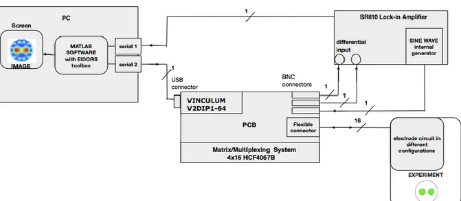
2.1. EIT system: Block Diagram 49
2.2 Hardware 52
2.2.1. Parasitic effects 60
2.2.2. Acquisition Strategy 69
2.3. Software 74
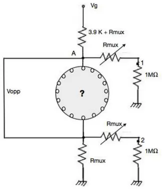
2.4. PCB Calibration 78
2.5. Forward Problem Simulation 80
2.6. Homogeneous Image Reconstruction: Saline Solution 83
3. Inhomogeneous Reconstructions of Various Objects
3.1. Image of Conductive and Insulating Objects 86
3.2 Results 101
4. Biological Sample Imaging
4.1. The Complex Admittivity Case 103
4.2. Biological Sample: Tissue Section 105
4.3. Human Sample: Skin 114
4.3.1 3D Imaging with Planar Electrode Array: Numerical Simulation 115
8 5. Conclusions 128 6. Future Work 131 References 133 APPENDIX: A. Printed Components
A.1. EIT System Components 143
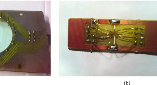
A.2. Circular Electrode Array 158
A.3. Planar Electrode Array 160
B. Data Acquisition Matlab Codes
B.1. Impedance Measurement Code 161
B.2. Calibration Code 165
B.3. Saline Solution Measurement Code
B.3.1 Acquisition of 16 Data for the comprehension of the reliability
of the Software in solving the forward problem 167
B.3.2 Acquisition of 256 Data for the comprehension of the reliability
of the Software in recreating images 171
B.4. Acquisition Code 174
C. Electrical Impedance Tomography EIDORS Codes C.1. Simulations
C.1.1. Forward Solving 180
C.1.2. Conductive, Insulating Objects 182
C.1.3. 3D Reconstruction of layers 183
C.2. Reconstructions
C.2.1. Saline Solution Reconstruction 185
C.2.2. 2D Protocol: Reconstruction of Various Object 187
C.2.3. 3D Protocol: Reconstruction of a Tissue Section 189
9
Chapter 1
1.Introduction EIT
1.1 Background
Estimating the conductivity inside a volume from electrical measurements on its surface is an imaging modality known as Electrical Impedance Tomography (EIT).
EIT belongs to a family of electromagnetic images modalities along with electrical capacitance tomography (ECT) [13] [14], electromagnetic tomography (EMT) [15], and magnetic induction tomography (MIT) [16].
The basic idea of EIT is to reconstruct the internal electrical conductivity distribution of the medium by measuring the electrical potential on its boundaries, where an array of electrodes is attached, while this is subjected to a sequence of low-frequency current patterns.
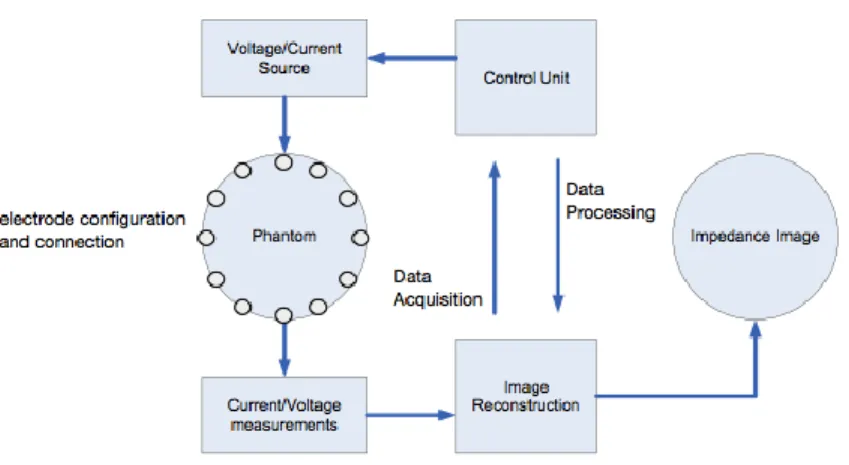
A typical EIT system is a compact set of equipment mainly consisting of a data acquisition unit comprising a current source, the electrodes and all the necessary drivers and amplifiers, a computer with the impedance reconstruction and visualization code on board.
EIT has quite long history starting from the interest in measuring electrical properties of tissues, but using electrical current to “probe” the tissue to reveal information about its integrity, density, cellularity rather than recording its inherent electrical characteristics. For example, as early as 1901, King applied electrical current to patients with hypothyroidism, describing the disease as a low impedance state [10], and over the next two decades electrical impedance measurements were performed on blood and other body fluids to help characterize them in health and in disease. In 1926, it was demonstrated that electrical impedance could be used to detect a breast tumor [7] and in the 1940 impedance measurements were introduced for the study of blood flow, impedance plethysmography [8]. Around this time impedance methods were also applied to nerve. In the following decade, Kenneth and Robert Cole, also helped researchers interpret impedance measurements in biological tissues by introducing simple circuit representations of
10
the body introducing the “Cole-Cole plots”, that continue to be used to this day. In 1967, Geddes and Baker reported the specific resistance of biological tissues including body fluids, blood, cardiac muscle, skeletal muscle, lung, kidney, liver, spleen, pancreas, nerve tissue, fat, and bone, nearly covering all the main organs within human body [20]. It has also been shown that electrical properties of malignant tissues are significantly different from those of normal and benign tissues. Surowiec et al. have reported that the electrical resistance of malignant tumors decreases by a factor of 20 to 40 with respect to normal or benign tissues [21].
Henderson and Webster are credited with producing the first medical image based on impedance on 1978 [9], they created the first impedance imaging system, the Impedance Camera to study the pulmonary edema. They used a two-dimensional matrix of 100 electrodes on one side of the thorax and a single large electrode on the other to produce a transmission image of the tissue. The instrument makes 100 spatially specific admittance measurements per frame at rates up to 32 frames per second. They applied a 100KHz AC voltage signal to a large electrode on the chest, and measured the current through an array of 100 small electrodes on the opposite side using a single channel. However, the assumption they made was not valid because they assumed electric currents traveled in straight lines, which is not true. This work was probably the first attempt at electrical impedance imaging.
Since then, many studies have been focused on the area of electrical impedance imaging, and many feasible approaches have been proposed including electrical impedance tomography (EIT), magnetic resonance electrical impedance tomography (MREIT) (fig. 1), and magnetic induction tomography (MIT).
A tomographic impedance image involving a reconstruction algorithm was realized in 1982 by Barber and Brown [11] [12] (Sheffield group). They used 16 electrodes around the thorax and a back-projection method of image reconstruction, obtaining the first published tomographic images.
During the last twenty years there have been many research programs and great number of publications in medical areas, and recently, significant advances have occurred in EIT. For instance the group of Cherepenin at all has published a 256 electrode system that provides a 3-D image of breast [5].
The technique of Electrical Impedance Tomography, which is focused on image reconstruction, has also garnered considerable engineering interest and remains an intense area of research. In
11
fact a 3D reconstruction engine developed for the EIT and Diffuse Optical Tomography Reconstruction Software (EIDORS) project [2].
In the past EIT was explored to become a generalized imaging modality. Though presenting lower signal to noise ratio [3] and lower spatial resolution [4] than other imaging modalities, EIT offers important strengths, such as high-speed data collection and soft tissue contrast which cannot be obtained from other imaging techniques. It has the potential for substantial impact on a number of clinical questions being a relatively low-cost technique [1].
12
1.2 Electrical Impedance Tomography as an Imaging Modality
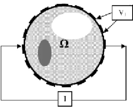
In Electric Impedance Tomography electric currents are injected into a body with unknown electrical properties through a set of contact electrodes at the boundary of the body (fig.1.1.a), and the resulting voltages are measured on the same electrodes. The objective is to reconstruct unknown electric impedance distribution within the domain. This impedance distribution is obtained by an estimation algorithm, which relies on an accurate model of the electrical interaction, based on these boundary data. The impedance distribution is represented by an image (fig.1.1.b) and constitutes the solution of the inverse problem, as explained in chapter 1.5.
(a) (b)
Figure 1.1: Electrical Impedance Tomography
(a) The EIT system developed by M.Cheney, D.Isaacson, J. C. Newell, 2000. It consists on 32 electrodes encircling the chest of a subject. (b) One „perfusion‟ image obtained.
Impedance is known as electric conductivity and permittivity in complex case. It represents the electric properties of the body under study, since the electric conductivity is a measure of the ease with which a material conducts electricity and the electric permittivity is a measure of how readily the charges within a material separate under an imposed electric field. Both of these properties have seen much interest in medical applications for many years, because different tissues, or even the same tissue in different physiological states, have different conductivities and permittivities.
13
The process of property estimation is highly nonlinear, ill-conditioned and ill-posed [6] and there are three principal difficulties in image reconstruction for EIT:
B. the relationship between the permittivity/conductivity distribution and electrical voltages is nonlinear [17] and the electric field is distorted by the material present.
C. the number of independent measurements is limited, leading to an underdetermined problem.
D. the inverse problem is ill-posed and ill-conditioned, making the solution sensitive to measurements errors and noise [18].
These are important factors limiting the quality of the image obtained.
EIT is an ill-posed inverse problem means that large changes in impedance at the interior of the object may result in only small changes to the electrical measurements on its surface, and thus the EIT reconstruction is not stable to data perturbation or model errors [19]. To detect small size impedance variations within the object, effectively providing good spatial resolution, we need to estimate a large number of conductivity or permittivity parameters in the inverse problem, which further reduces the stability of the solution algorithm. Therefore, there is a trade-off, in the general case, between spatial resolution and stability. The fact that the electrical properties depend nonlinearly on the measured quantities makes this trade-off even more difficult.
The ill-posedness of the problem makes it unlikely that EIT images, even with many electrodes, can achieve resolution comparable to that of computed tomography (CT) or magnetic resonance imaging (MRI) images.
We can explain better this concept: „Soft-field‟ modalities such as EIT, are intrinsically different compared to „Hard-field‟ techniques like X-rays computed tomography, widely established in high resolution imaging. In an CT scanning process, parallels beams of X-rays are guided into the body under test from a suitable source while some detectors measure the attenuated beams as these emerge from the body. Since the procedure is repeated, rotating both sources and detectors around the body under test, in sequence, images of the attenuation coefficient
14
distribution inside the body are developed using analytic algorithms. This appears to be extremely efficient for this particular reconstruction problem in terms of its computational speed and the spatial solution of the image. This is mainly because the X-rays absorption at any point inside the body is completely independent from any other point. This is in fact a linear problem which leads to sparse and well-conditioned sensitivity matrices and very large data sets.
On the other hand, in EIT, being the current distribution inside the body function of the spatial distribution of the electrical properties, an electrostatic representation is most appropriate, describing the field throughout the body using the Laplacian equation [5]. As the field is modified throughout the body, the measured potential values at a given boundary location under a given excitation geometry is a nonlinear function of the distribution of the electrical parameters.
The relatively poor spatial resolution of the reconstructed images in impedance tomography is often quoted as its major disadvantage, compared with other already established tomographic scanners. To this respect, it must be clarified that the motivation for EIT is somewhat different from that of a conventional imaging modality. Despite its limited resolution, its task is to provide a portable and efficient imaging tool optimized for speed and contrast. In an abstract way, the reconstructed image can be seen as a source of information aiming to answer clinically-relevant questions about the interior electrical properties of a particular volume, rather than providing accurate morphological information. Depending on the particular application and resolution specifications, EIT can sometimes provide the optimum cost-effective solution.
EIT has many advantages over other medical imaging techniques. It is a non-invasive, and it does not expose the patient to X-rays or any other radioactive materials. It is a safe for long term monitoring. In addiction EIT, combined with other medical imaging techniques can provide increased diagnostic accuracy. For example, if X-rays can only detect breast tumor that have an X-ray absorption that differs significantly form that of the normal breast tissue, EIT is based on the contrast in electrical properties of the tissue and can be used to find or distinguish tumors that are undetectable or indistinguishable by mammography [22].
15
1.2.1 Clinical Applications
Electrical Impedance Tomography, as said, is a new type of technology still under heavy development in recent years.
Two different modalities of images can be obtained as a result of the inverse problem solution and reconstruction: The absolute and differential ones.
Absolute imaging attempts to quantify the actual value of conductivity or permittivity inside an object. For such techniques, it is assumed that the properties of object do not change during the measurement process, so sometimes is also called static imaging. The technique is often used for characterizing biological tissue [48] [54] [55].
Instead, the aim of differential imaging, also known as dynamic imaging, is to reconstruct a change in conductivity rather than an absolute value, it reflects the change in the distribution of conductivity over the cross section. Dynamic EIT is of interest in studying physiological processes which modify the electrical conductivity of the body.
This technique has been used for imaging temporal phenomena in medical applications, such as impedance changes during respiration [23] [49]. This Thesis is especially concerned with absolute impedance imaging.
Other possible clinical applications of EIT include monitoring cardiac [25] and brain function [58] (fig. 1.3), detection and quantification of intraperitoneal fluid [26], detection and characterization of tumors [27] [56] [57], detection acute cerebral stroke [30], monitoring cancer ablation procedures and hypertermia [28] [29] [31] (fig.1.2), monitoring the freezing extent in cryosurgery [47], monitoring the change in conductivity of the tissues during the process of electropermeabilization in electroporation [59], studying the emptying of the stomach [32] [50], studying pelvic fluid accumulation as a possible cause of pelvic pain [33], quantify severity of premenstrual syndrome by determining the amount of intracellular versus extracellular fluid [34], determining the boundary between dead and leaving tissue [35], and building forward models for bioelectric field inverse problems such as Electro/Magneto Encephalography (E/MEG) [36] [37], and Electro/Magneto Cardiography (E/MCG).
A variety of non clinical applications of EIT is also possible. These include imaging multi-phase fluid flow [38] [39], determining the location of minerals deposits in the earth [40][41], tracing
16
the spread of contaminants in the earth [42] [43] [44], non-destructive evaluation of machines parts [45], and control of industrial processes such as curing and cooking [46].
(a) (b)
Figure 1.2: The EIT group in Moscow produced 3-D tomographic images of in vivo breast tissue
from women with different hormonal status using a circular grid of 256 electrodes, 2010.
(a) Shows a patient under examination. (b) The EIT system (http://www.nbmdi.com/products/).
Figure 1.3: The UCL group (Departments of Medical Physics, University College London and Clinical Neurophysiology 2010, University College Hospital, London, UK) performed a number of measurements from human volunteers who were subject to visual, motor, and somatosensory stimuli to assess the applicability of
17
1.3 EIT Theory
Electrical impedance methods are based on measurement of the electrical impedance, i.e., the modulus of the full complex resistance, of the human body or tissue.
All impedance methods relay upon the basic principle that if an alternating current is applied to a substance, energy will be dissipated as it travels through it, thus producing a measurable voltage. Moreover, the timing of the oscillations in the measured voltage will be out of phase with those of applied current.
The figure 1.4 helps to illustrate how the impedance measurements work. An alternating electrical current of known frequency, amplitude and timing, (i.e., the waveform crosses the x-axis at a specific time) is applied to a tissue. As the electrical current travels through the tissue, due to the tissue‟s inherent resistance, it loses energy, thus reducing the amplitude. Moreover, the timing of the resultant voltage alternations is slightly delayed, with it is no longer crossing the x-axis at the expected time, due to the substance‟s inherent capacitive and inductive characteristics.
Figure 1.4: Basic concept of electrical impedance testing.
Electrical current of a known frequency, amplitude is injected into a tissue. The tissue impacts the applied electrical current, reducing the measured voltage‟s amplitude, secondary to the tissue‟s resistance and slightly altering its timing, secondary to the tissue‟s capacitance. The changes in electrical current flow reflect the properties of the
tissue and thus can reveal information about tissue health or pathology.
Impedance can be described mathematically by Ohm‟s Law, which states that, for pure resistive circuits, without capacitors and inductors:
18 V = R I (1.3.1)
where V, represents voltage, R, the resistance and I, the current.
For the complex representation of Kirchoff‟s laws [18], such elements are included and the
equation becomes:
V = Z I (1.3.2)
where Z represents the complex impedance of the circuit, a combination of its inherent resistance (R) and its reactance ( X) , where X is a purely imaginary component. There are two types of reactance: the capacitive reactance ( ) and the inductive reactance ( ). Z is a vector, expressed as a complex number, composed of its resistance and two forms of reactance in combination:
Z= √ (1.3.3)
Fortunately, in medical applications this equation can be simplified bi ignoring the XL term,
since the inductance is believed to play a minimal role in standard bioimpedance measurements and the term can be simply written as X.
Whereas the above equation can be applied to direct current circuits, it is most applicable to circuits utilizing alternating current, since in direct current circuits the current will simply stop following across the capacitor once it is fully charged; however, in alternating current circuits, current will flow indefinitely since it is constantly shifting direction.
We can also calculate the phase angle via standard trigonometric relationships by the formula:
= arctan ( X / R) (1.3.4)
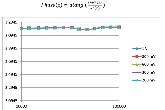
Thus, when discussing bioimpedance measurements in biological tissues, we should consider always all the components of the measured voltages mainly the phase angle which reflects to behavior of the sample we are studying. That was why, in this thesis, we used a Lock-in amplifier as measurement system and in every data acquisition file we measured all the voltage components.
19
In the literature two different electrode setups are used to measure the electric properties of biological materials: the two-electrode method and the four-electrode method.
In principle it could be supposed that tissue impedance could be measured by a couple of electrodes attached to the surface of the sample under study (two-electrode approach). Both of electrodes are used to inject the current and to measure the voltage drop (fig.1.5 a). The voltage in this case is measured across the entire circuit (fig.1.5 b). However the electrode-electrolyte impedances are in series with the sample impedance, and, therefore the measured impedance is the sum of the three impedances (ZX + Ze1+ Ze2). Unfortunately these parasitic impedances are
sufficiently large to disturb the measurements, especially at low frequencies.
(a) (b)
Figure 1.5: two-electrode method
(a) In the two-electrode approach, current is injected at the same location where the intervening voltage is measured. (b) Equivalent Circuit.
Because of that, generally, two pairs of electrodes are used (four-electrode approach): the outer (current) electrodes, and the inner (voltage) electrodes. The current from the source passes through the sample. Voltage electrodes of known separation are placed in the sample between the current electrodes (fig.1-6 a b).
20
(a) (b)
Figure 1.6: four-electrode method.
(a) In the four-electrode approach, current is injected separately. (b) Equivalent Circuit.
In EIT the conventional way of obtaining impedance measurement of an imaging domain, that could be an object as an biological sample or a part of human body, is to surround it with a certain number of source and probing electrodes as schematically shown in fig. 1.7. There are a number of variation of EIT system that depend on whether one injects current and measures voltages, and on whether one uses the same or different electrodes for this purpose, but most bioimpedance applications use the tetrapolar approach, since, it can help isolate an area of interest and being I and V independent, the polarization on the current electrodes has no influence on the voltage difference between the voltage electrodes.
21
In choosing the features of the system it is fundamental to consider the number of electrodes with respect to the resolution one can obtain. It has been shown in [91] that the resolution of an EIT system improves if one uses electrodes that fill as much as of the outermost surface as possible, that because it has been shows that the signal-noise ratio is approximately proportional to the square root of the fraction of the available circumference covered with electrodes [92] and this suggest using large electrodes.
The theory behind electrical impedance tomography is that by applying a constant current across a material, the voltage distribution resulting on the surface will reflect the internal impedance distribution. However, intuitively one will understand that multiple impedance distributions can produce the same voltage distribution at the surface. Therefore the system is stimulated in multiple manners to constrain the possible impedance distributions. Figure 1.7 shows a simple EIT diagram with 16 electrodes around the perimeter of a circular medium. In this setup the current, I, is applied across a pair of electrodes on opposite sides of the core while the voltage distribution, Vi, is measured between each set of neighboring electrodes. After the voltage around the entire perimeter has been measured, the current drive electrodes are rotated to the neighboring electrode, such that they remain opposite, and the voltage at all electrodes is measured once again. This process continues until 256 sets of voltage measurements are obtained.
22
The governing equation for the voltage field produced by placing a current across a material is shown below in Equation 1.3.5.
(1.3.5)
Where and are the electric conductivity and permittivity of the medium, is the electric potential, is the frequency. The sum of conductivity and permittivity is the complex admittivity of the medium, the impedance.
The EIT inverse problem is simply a system stimulation problem. The stimulation and resulting effect (injected current i and measured voltage V) are known, but the internal physical system is unknown (impedance distribution). The difficulty in solving this problem lies in the nonlinearity that arises in impedance itself, because the potential distribution is a function of the impedance it-self, and we cannot easily solve equation 1.3.5 for impedance [63].
For solving the EIT problem, it is important to consider the distribution of the electrodes and the fact that they cover a part of the surface under study. That because the presence of highly conductive electrode material on the surface of the body provides an effective short circuit for the applied current, which may reduce the current density at the interior of the body. We need therefore to mathematically model their presence. A sequence of electrode models was first introduced be Cheng.et al. in [92]. These models in order of increasing fidelity (and complexity of the problem), are generally known as the continuum, gap, shunt and complete models.
The continuum model assumes the current density on the entire outer surface as known, but it is a poor model for real experiments because we do not know the entire current density, but in practice, we only know the currents that are sent down wires attached to electrodes, which in turn are attached to the body. The gap electrode model is a refinement of the continuum model which accounts for the discreteness of the electrodes. Electrodes are mathematically represented as a set of disjoint subdomains of the boundary. The current density is assumed to be nonzero and constant under an electrode, and zero in the gaps between electrodes. The shunt model accounts that metal electrodes provide a low-resistance path for the current. Modeling in addiction the
23
contact impedance between the electrode and the body results in the complete model, that is superior to the previous models because it predicts the measured data more accurately [93].
1.3.1 Different Modalities for Electric Measurement of Impedance in EIT
An EIT system belongs to the class of the Pair drive instruments.
Pair drive instruments have a single current source and sequentially apply electrical currents to the body using a pair of electrodes. Voltage differences resulting from the stimulus are then measured between pairs of the remaining electrodes.
The way in which the driving pair is switched and the voltage measurements are collected in this type of instrument varies. Some of the most common configurations in medical applications use the adjacent, the cross and opposite methods.
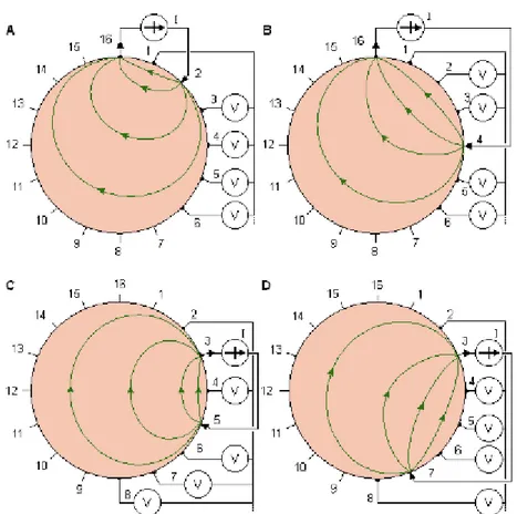
Brown et al. suggested a method whereby the system sequentially applies electrical currents to the body using a pair of adjacent electrodes [1]. While current is applied to the body, voltages between adjacent non-current-carrying electrodes are measured. This procedure is repeated, applying current between each pair of adjacent electrodes to obtain a voltage data set.
Fig. 1.6 illustrates the application of this method for a circular volume conductor with 16 equally spaced electrodes. The current is first applied through electrodes 1 and 2 (see Fig. 1.8 a). One then measures the voltage using electrode pairs 3-4, 4-5, ..., 15-16. From these 13 voltage measurements the first four measurements are illustrated in Fig. 1.6 a. All these 13 measurements are independent. The next set of 13 voltage measurements is obtained by applying the current through electrodes 2 and 3, as shown in Fig. 1.8 b. This method, because the current is driven mostly in the outer region of the object, is very sensitive to conductivity contrasts near the boundary and almost insensitive to central contrasts, making the ill-posedness of the inverse problem even worse [65].
24
Figure 1.8:Adjacent method of impedance data collection illustrated for a circular volume conductor and 16 equally spaced electrodes.
(A) The first four voltage measurements for the set of 13 measurements are shown. (B) Another set of 13 measurements is obtained by changing the current feeding electrodes.
A more uniform current distribution is obtained when the current is injected between a pair of electrodes which are more separated from each other. Hua et al. suggested such a method called the cross method [64].
In the cross method, first one chooses two adjacent electrodes for current and voltage reference electrodes (for instance 16 and 1 in Fig. 1.9 a, respectively). The current is injected through electrode 2, and the voltages is measured for all other 13 electrodes with the aforementioned electrode 1 as the reference (the first four voltage measurements are again shown in Fig. 1.9 a). The current is then applied through electrode 4, and the voltage is again measured for all other 13 electrodes with electrode 1 as the reference, as shown in Fig. 1.9 b. One repeats this procedure using electrodes 6, 8, . . . 14; the entire procedure thus includes 7 × 13 = 91 measurements. The measurement sequence is then repeated using electrodes 3 and 2 as current and voltage reference electrodes, respectively (see Fig. 1.9 c). Applying current first to electrode 5, one then measures the voltage successively for all other 13 electrodes with electrode 2 as a reference. This procedure is repeated again by applying current to electrode 7 (see Fig. 1.9 d). Applying current to electrodes 9, 11, ..., 1 and measuring the voltage for all other 13 electrodes with the afore-
25
mentioned electrode 2 as a reference, one makes 91 measurements. The cross method does not have as good a sensitivity in the periphery as the adjacent method, but has better sensitivity over the entire region [65].
Figure 1.9: Cross method of impedance data collection. (a), (b), (c), (d): The four different steps of this procedure.
As an alternative, Hua et al. introduced another method called the opposite method [64]. Fig. 1.10 illustrates the application of this method for a circular volume conductor with 16 equally spaced electrodes. In this method one injects current through two diametrically opposed electrodes (electrodes 16 and 8 in Fig. 1.10 a), and uses the electrode adjacent to the
current-26
injecting electrode as the voltage reference. The next set of 13 voltage measurements is obtained by selecting electrodes 1 and 9 for current electrodes (see Fig. 1.10 b). The current distribution in this method is more uniform and, therefore, has a better distribution of the sensitivity than the cross method [65].
Figure 1.10: Opposite method of impedance data collection.
(a),(b) : The two different steps of this procedure.
1.4 The Inverse Problem
The inverse, or reconstruction, problem is to obtain an approximation to the conductivity/permittivity map in the interior from the boundary measurements. The inverse, or reconstruction, problem is to obtain an approximation to the conductivity/permittivity map in the interior from the boundary measurements. In 1932, Hadamard attempted to describe the generic properties of such problem which arise from physical and natural phenomena [35].In these, a given set of observations is always uniquely mapped to a given set of admissible rational
27
solution. Thus, according to Hadmard, in a well-posed problem for any set of rational observation
(a) A solution consistent with the observations exists.
(b) The solution is unique.
(c) The solution depends continuously on the observations.
In Hadmard‟s meaning, problems failing this criteria could have never arisen from a physical system, and somehow these would have been misinterpreted and posed incorrectly, hence the name ill-posed. Despite this, the inverse admittivity problem is undoubtedly ill-posed, because a small change in conductivity/permittivity next to a physically conductive area will have a smaller effect on the boundary voltages. The relationship between the admittivity changes and the corrisponding differential boundary voltages is also not linear, and although some naturally imposed constraints may somehow suggest, though not guarantee, the validity of the first two criteria, it certainly fails the third one, because even small perturbations in the measurements can lead to wild oscillations in the solution.
In order to solve the inverse problem a consideration should be done: In principle, measuring both the amplitude and the phase angle of the boundary voltages can result in images of the electrical conductivity and permittivity distributions in the interior volume. Despite this, the fact that electrostatic fields are ideally required, alternating current patterns are often preferred in order to avoid polarization effects. In the frequency range lower than 100 KHz, the magnetization component of the current is negligible and the phase angles are maintained relatively small, thus usually the real part of the voltages is a few hundred times greater than the imaginary. In absence of phase angle readings in the data, only the conductivity (or equivalently the resistivity) distribution can be reconstructed. Said that, if the difference between the conductivity of an object and its surroundings is small, this nonlinear problem can be approximated to a linear one in the form:
28
where V ϵ is the measurement vector of the boundary voltages, J ϵ is the sensitivity
matrix or Jacobian and G ϵ is the vector representing the impedance distribution, m is the number of the independent measurements, and n is the number of the conductivities in the area of interest.
To obtain the conductivity map inside the volume equation (1.4.2) must be inverted for
G V (1.4.2)
Equation (1.4.1) and (1.4.2) show the forward and inverse processes of the image reconstruction, respectively.
Obviously, to reconstruct an EIT image from the voltage measurements, (1.4.1) has to be solved. However there are several difficulties associated with the inverse of the sensitivity matrix J: being generally not square, it has no direct inverse and a pseudoinverse of the Jacobian is required; being ill-posed and since there are fewer independent measurements that unknown conducivity values, many alternative images are possible; being ill-conditioned, i.e., its condition number of the sensitivity matrix, defined as the ratio of largest singular value of the matrix to its smallest one, is typically very large, result in magnification both of measurement and numerical errors in the reconstructed image.
When approaching an ill-posed problem, the tendency is to replace it with one of which is somewhat different but „less ill-posed‟. Ill-posed problems „suffer‟ from an inherent shortage of information, therefore instead to attempt to solve the original problem one often opts to solve a similar one which is less demanding or one for which more information is available. This transformation can be achieved in a variety of ways, with regularization amongst the most popular ones. Regularization is essentially a means for providing to the inverse problem some prior information about the solution, and in this sense it can be viewed as a constraint preserving the existence and the uniqueness but also the stability of the solution. From another perspective, regularization can be interpreted as a means to trade-off the influence of measurements on the solution against its compliance with the prior assumptions.
The most majority of existing algorithms for image reconstruction in EIT follow these fundamental steps:
29 a) Find the Solution for the Forward Problem. A forward solver capable of predicting the voltages on electrodes, at least as accurately as the measured data, for a given conductivity distribution is essential for EIT reconstruction.
b) Calculate of the sensitivity matrix, which is the Jacobian of the discrete forward operator. The forward solver is called to compute the voltages on the electrodes and the internal electric potential is required to assemble the Jacobian matrix for the inversion [90].
c) Invert of the sensitivity matrix. The voltages measurements are then converted to permittivity image by solving a regularized inverse model typically formulated on a finite-element mesh.
d) Reconstruct of the image.
Many reconstruction algorithms have been proposed by a number of research groups. These approaches fall into several different categories. I outline several of the different approaches and then in 1.4.1 section describe in more detail the methods I used to make the images that accompany this Thesis.
The diagram in figure 1.11 gives a brief overview on the types of the already available reconstruction algorithms for the EIT problem. These are generally divided in probabilistic-statistical methods (Kipio, Kolehmainen, Somersalo, Vauhkonen) [81] [82] [83] [84], deterministic methods based on linearization ( Allers, Barber and Brown, Blue, Calderón, Cheney, Goble, Isaacson, Newell ) [66] [67] [68] [69] [70] [71] [72] [73], and deterministic nonlinear inversion methods (Berryman, Webster, Wexler, Lionheart, Vaukhonen, Borsic, Arridge) [74] [75] [76] [77] [78] [79] [80].
The linearized algorithms, suitable for solving the linearized inverse problem, are subdivided in direct methods that use a single regularized step, such as Tikhonov regularization [85] and one-step Newton methods [48] [86] [87] [88], and iterative methods which regularize by iteration, such as the conjugate gradients algorithm [89]. The nonlinear algorithms on the other hand, capable of reconstructing high-contrast inhomogeneities by tackling the nonlinear inverse problem, are mostly iterative, typically Newton-type with a linear regularized step.
The images in this Thesis were made with a one-step Newton method (NOSER) that is close to an approximate linearization and it has been preferred to iterative methods for its lower computational time. This I discuss in more detail below in paragraph 1.5.
30
Figure 1.11: Reconstruction algorithms for EIT.
1.5 Algorithms for the Ill-posed Problem
For solving the EIT problem I used EIDORS, that is a freely available software officially released under GNU General Public license by Vauhkonen [94] at the second half of 2000, as a complete package for two dimensional EIT problems. Being most medical problems fundamentally three dimensional, in 2002 Polydorides and Lionheart released a free toolkit of Matlab routines which can be employed to solve the forward and inverse EIT problems in three dimensions. In order to tackle the nonlinear and ill-posed problems, EIDORS employs the Finite Element Method (FEM) to solve the forward calculation. The finite element solver included in the toolkit uses the complete electrode model to compute boundary problems involving models with first-order triangular and tetrahedral elements. Simple files with primitive commands define the geometry of the desired domains comprising vertices (nodes) and simplices (vertices). These are imported into ready-available mesh generators, such as NETGEN [127]. In order to solve the inverse problem, EIDORS employs regularized Newton‟s methods and the result is a set of
31
impedance values, which correspond to the measurements by the electrodes. Below I describe the mathematical model for EIT. The model involves some of the theory that underlies the design of the EIT system utilized for this Thesis, and then I focus on discretization and finite element formulation, the forward computation, the calculation of the Jacobian matrix and, finally, on the algorithm used to make the images accompanyingthis Thesis.
1.5.1 Mathematical Model of the Physical System
In order to model the physical system, an accurate model of volume is imperative. This must respect the dimensions, the boundary geometry and the structural characteristics of the physical volume. In addition, the boundary electrodes must be accurately modeled.
The mathematical model comes from the Laplacian equation derived from Maxwell‟s equations from electro-magnetics. In the following equation E is the electrical field in the interior of the volume, B the magnetic field, the charge density, j the current density, v the outward unit normal vector, c the speed of light and the dielectric permittivity in vacuo. For a conductive isotropic volume Ω enclosed by boundary , Maxwell‟s equation state that the flux E through a closed surface equals the total charge density inside divided by .
(1.5.1)
In addition, the linear integral of E around a loop is equal to the negative rate of change the flux of B through the loop, yielding
32
the flux B through a closed surface is equal to zero,
(1.5.3)
and the integral of B around a loop is equal to the current flowing through the loop plus the rate of change of the flux of E through the loop divided by a constant , yielding
(1.5.4)
In EIT the excitation conditions are quasi-static as the driving patterns are time-harmonic AC signals at a low frequency . However, if the measurements for each pattern are thought to be collected instantaneously, then static condictions can be assumed. In effect, the magnetization components can be safely neglected, hence
and
(1.5.5)
Using these, equation (1.5.2) becomes
(1.5.6)
From vector calculus theory, when the curl of the vector E is equal to zero, then there exists a scalar u whose gradient is equal to that vector, in particular
(1.5.7)
When „static„ current patterns are injected, under the assumptions (1.5.5), equation (1.5.4) becomes
33
In these conditions the current density j can be assumed to be time invariant. If is the n‟th current pattern driven into volume, from a boundary electrode surface s then
∫ (1.5.9)
From the charge conservation law, if S is the surface of
∫ (1.5.10)
the charge in the interior of the volume can be expressed as a volume integral of the charge density as
∫ (1.5.11)
Combining (1.4.12), (1.4.10), and (1.4.11) yields
(1.5.12)
which is basically another expression for the charge conservation theorem, according to which the flux of the current flowing through a closed surface is equal to the negative rate of change of charge density in the interior. Since there are no current sources in the interior of the volume and
E does not change with time, the right hand side of the equation (1.5.) can be set to zero
(1.5.13)
In the linear isotropic medium the current density and the electric field are related by the approximation
34
where is the electric conductivity, the electrical permittivity and the complex admittivity of the medium. Substituting (1.5.14) into (1.5.13) leads to
(1.5.15)
which combined with ( 1.5.7 ) yields the Laplacian partial differential equation
(1.5.16)
(1.5.17)
This nonlinear partial differential equation representing the electrodynamics of EIT is known as Governing Equation of EIT and has an infinite number of solutions. Boundary conditions required to restrict these solutions can be applied to specify the value of certain parameters on the surface. These may be either the potential at the surface (Dirichlet conditions) and/or the current density crossing the boundary (Neumann conditions).
The mixed Dirichlet and Neumann boundary conditions accompanying the Laplacian equation (1.5.17) are formally know as the complete electrode model (CEM), which, as said, is superior to the previously used continuum, shunt and gap models because of its better resemblance to the physical system, encapsulating the contact impedance of the electrodes. If is the subset of the surface of the volume underneath the electrodes, then the associated current density is
on (1.5.18)
while for the rest of the surface ,
on (1.5.19)
In addition, for each of the electrodes the integral of the current density over the whole electrode surface s is equal to the total amount of current flowing to or from that electrode,
35
∫ l (1.5.20)
where L is the number of the electrodes in the system (Neumann Boundary Condition). Finally, the value of potential measured on the l‟th electrode is equal to the sum of the potential on the boundary surface underneath that electrode and the potential drop across the electrode‟s contact impedance ( Ω ∕ ) (Dirichlet Boundary Condition)
l (1.5.21)
The model has been shown to have a unique solution when the charge conservation theorem
∫ ∑ (1.5.22)
is considered, and a choice of ground is made,
∫ ∑ (1.5.23)
36
1.5.2 Discretization and Finite Element Formulation
When the problem is solved numerically, the model of the physical system must be discretized, requiring an approximate formulation of the problem. The accuracy of the approximation is strongly dependent on the smoothness of the analytical solution to the Laplacian equation (1.5.17), which in turn depends on the smoothness in the measurements. Piecewise assumptions about the regularity of the forward solution (potential) and the input data (admittivity) can be formulated considering classes of discrete functions with specific integrability properties. Usually the transformation from the continuum domains and integral operator functions to the discrete domains and matrix operators is achieved by some numerical integral approximation methods such as the Galerkin methods [95]. In the discretization process it is essential that both the solution and the data are taken to be functions over some spaces. Despite using only finite sets of parameters, infinite dimensional spaces are preferred as they reflect the fact that behavior resemblance between the physical-continuous system and its discrete model becomes higher as the number of parameters increased. In EIT, infinite dimensional Hilbert spaces are often used to represent admittivity distributions and boundary measurements.
In this Thesis, In this Thesis, for the finite approximations of the forward problem, the Galerkin three dimensional formulation is used [60]. In this, the admissible measurements and the solutions are considered to belong to the Hilbert spaces, and the forward nonlinear operator is formalized as
(1.5.24)
hence given a model, the forward operator F can also thought of as a Neumann-Dirichlet operator associated with .
The finite element formulation for EIT, first discretizes the medium under analysis into a finite number of elements collectively called a finite element mesh. Within each element the nodal values are approximated by shape functions (interpolation functions).
Before showing how the Galerkin approach develops into the EIT forward solver, the weak-variational form of the problem must be derived first. If is the required weak solution to the
37
problem, or better defined as a finite dimensional approximation for the weak solution and are some piecewise linear basis functions with limited support such that
{ (1.5.25)
then
∑ (1.5.26)
where is the value of the potential at vertex i and n the number of vertices in the model. From (1.5.26) it is clear that is a linear combination of the functions weighted by the vector. Based on equation (1.5.26), the array of FEM parameters U must be evaluated such that
∑ ∭ j=1, …, n (1.5.27)
For FEM derivations the discrete conductivity distribution vector is taken as
∑ (1.5.28)
where
{ (1.5.29)
are piecewise constant functions or, better, the nodal basis functions of the finite element mesh. Combining the Laplacian (1.5.17) with equation (1.5.26) leads to
∭ i=1, …, n (1.5.30)
38
∭ ∬ i=1, …, n (1.5.31)
where
(1.5.32)
and s is a boundary surface measure.
According to the Galerkin method, equation (1.5.31) must be applied to each of the elements in the model. For the needs of the derivation, a finite element model with k first-order tetrahedral elements, n vertices and L boundary electrodes is assumed. For an element underneath the electrode l, let be the volume of the element and its triangular face shared with the electrode. Equation (1.5.31) for the particular element becomes,
∭ ∬ (1.5.33)
for i=1,...,4 and plugging in the boundary condition (1.5.20) yields,
∭ ∬ (1.5.34) where is the contact impedance of the electrode l and the potential measured on it.
Substituting from (1.5.26) leads to
∭ ∬ (1.5.35)
with i, j=1, ..., n.
Generalizing equation (1.5.35) for the n‟th element, the global conductance matrix A is assembled by evaluating the following entries for each of the elements. These entries formalized
39
as local matrices , and arise from the various factors of (1.5.35) and depend on the actual location of the element. The local matrices are
∭ i, j (1.5.36) ∬ i, j (1.5.37) ∬ i, j (1.5.38) { i, j (1.5.39)
where are the four vertices in each element and is of the face of the electrode.
For the exact derivation of the local matrices, I suggest referring to [95]. For a finite set of current patterns, the forward problem is formulated as a system of linear equations
( ) ( ) ( ) (1.5.40)
where is U the nodal potential distribution and the potential values on the boundary electrodes. Before the system (1.5.40) can be solved, the additional conditions (1.5.41) (1.5.42) must be imposed in order to preserve the existence and uniqueness of the forward solution [93]. If I is the value of current injected by l‟th electrode, then for a set of k driving current patterns
( ) (1.5.41)
40
∫ ∑ 0 (1.5.42)
Given a finite element model with known admittivity distribution and a set of current patterns, the potential at the vertices of the model and the boundary electrodes can be calculated from equation (1.5.40). This process is referred as the forward computation. Expressing (1.5.40) in a more condensed form, the forward problems becomes
(1.5.43)
with u = ( U ) and b = ( 0 having an algebraic solution
(1.5.44)
In contrast to the inverse problem, this is a well-posed, easy to solve problem because the coefficients matrix A
- is very sparse due to the limited support in the elements of the model - is square and full-rank, therefore the solution is unique
- is symmetric and so is its inverse, enabling the decomposition of A in smaller factors whose inverse is easier to compute
41
1.5.3 Forward Computation
In general, the forward problem can be solved either directly or iteratively. It has been noted that, being a finite approximation weakly depending on the quality and smoothness of the model, the forward problem should be solved iteratively, as EIDORS does. Consequently, trying to solve the problem „ exactly „ has no impact on the quality of the outcome, as it bears no significance in trying to „ reproduce „ the data more accurately than they can actually be measured. The problem must be solved to a tolerance compatible with the quality of the actual measurements.
One of the most suitable iterative schemes for the forward problem is the linear preconditioned conjugate gradients ( PCG ) iteration. This iterative algorithm generates a sequence of solutions which minimize the least square residual
argmin (1.5.45)
and it requires the matrix A to be positive-definite in order for the iteration to be able to converge. The algorithm is classified under low-storage numerical techniques, because it avoids the computation of large components which are computationally expensive to store and handle. The properties and special characteristics of the linear PCG iteration are well established and documented in [96] [97] [98] [99] [100].
If M is a proper preconditioner, the modified forward problem becomes
(1.5.46)
which has solution identical to the original problem, where, however, only this time the convergence depends on the properties of the matrix than A alone. The matrix M must be
positive-definite and well-conditioned, so that its inverse can be easily computed. The preconditioner is selected in a way that
42
where I is the identity matrix. Setting an initial estimate of the potential distribution , the resulting residual vector and an initial ( steepest descent ) search direction , the PCG iteration is described in figure 1.12.
Figure 1.12: The preconditioned CG iteration. The scalar parameter denotes the tolerance
Usually the first search direction is along the steepest descent, while the iterative solution is obtained by stepping distance towards the current direction . The characteristic properties of the CG iteration can be summarized considering two successive iterations i,j. In these the residuals are M-orthogonal or M-conjugate,
(1.5.48)
the residual of the one iteration and the direction vector of the other are M-conjugate
43
and the directions are A-conjugate
(1.5.50)
1.5.4 Calculation of the Jacobian Matrix
When the admittivity is purely real, then any given set of low-frequency current patterns give rise to a purely real set of potential measurements at the boundary. Calculating the Jacobian for a distribution , if F ) are the boundary measurements in response to , then the real discrete linearized forward problem is
( ) F ) (1.5.51)
Where is the perturbed admittivity distribution and V the boundary measurements with respect to . By definition, the Jacobian is the discrete derivative of the nonlinear function which maps the perturbations of the solution to perturbation on the boundary data.
(1.5.52)
Denoting
( ( ) ( ) ( )) (1.5.53)
the vector of the boundary measurements corresponding to k driving current patterns, the Jacobian matrix J has the form
44 [ ( ) ( ) ( ) ( ) ] (1.5.54)
where k is the number of degrees of freedom in the model. The Jacobian is a linear, compact and positive operator on infinite Hilbert spaces. Furthermore, being a compact operator it has a discontinuous inverse, causing to be unstable against variations in the data, effectively violating Hadamard‟s third criterion for well-posedness.
For two-dimensional models the Jacobian is calculated using its definition (1.5.54). In this procedure, each of the elements is in turn perturbed by a small amount and then, solving the forward problem, the perturbation caused on the boundary measurement is calculated.
However, when the finite element models are three-dimensional with a large number of degrees of freedom, this method is extremely inefficient and is normally avoided. Following an adjoint problem formulation, the Jacobian can be calculated quite efficiently as the dot product of the current and measurement fields (these hypothetical fields can be calculated when the measurement patterns are considered to be current patterns) with the integrals of the gradients of the shape functions over each element [101] [86]. From the weak form of the Laplacian, as obtained by Green‟s second identity, then
∭ ∬ (1.5.55)
In particular for w = u the power conservation formula becomes
∭ ∬ ∑ ∬ ( )
(1.5.56) hence
45
∭ ∑ ∬ ∑ (1.5.57)
This simply states that the power input is dissipated either in the domain Ω or by the contact impedance layer under the electrodes. Taking perturbations and , with the current in each electrode held constant, and ignoring second order terms yields
∭ ∭
∑ ∬ ( ) ( ) ∑ (1.5.58) On the l‟th electrode
( ) (1.5.59)
Combining (1.5.59) with the weak formulation (1.5.55) using w yields
∭ ∬ ∑ ∬ ( ) ∑ ∬ ( ) ∑ (1.5.60)
Noting that the second and third terms on the left hand side cancel, and the fourth is simply 2∑ then
46
Equation (1.5.61) gives the total change in power. To get the change in voltage on a particular measuring electrode m when a current pattern is driven into the volume, the associated „ measurement pattern potential ‟ must be calculated. Note the distinction between the current potential ‟ and the measurement potential ‟ .
Applying the power perturbation formula (1.5.61) to and then subtracting gives the familiar formula
∭ (1.5.62)
where is the m‟th measurement under the d‟th current pattern. To calculate the Jacobian matrix one must choose a discretization of the conductivity. This can be taken either as piecewise constant, linear or even nonlinear on simplices on any other chosen polyhedral domain. Taking to be the characteristic function of the k‟th simplex, then for a fixed current pattern
∭ (1.5.63)
From equation (1.5.63) the similarity in the definitions of the Jacobian and the global conductance matrix is obvious, as they both involve the integrals of the inner products of the gradients of the shape functions over each element. Every row of the Jacobian matrix corresponds to the sensitivity distribution inside the model with regards to the particular measurement and the current pattern.
1.5.5 Inverse Regularized Solution
In order to solve the inverse problem, I choose a direct method, which calculates an „exact‟ regularized inverse of the Jacobian which is subsequently used to obtain the regularized solution in a single step.