Comparison between hydraulic and hydrologic routing models under different scenarios of cross-sections geometry availability

(1)

POLITECNICO DI MILANO

Department of Civil, Environmental and Land Management Engineering

Master of Science in Civil Hydraulic Engineering

COMPARISON BETWEEN HYDRAULIC AND

HYDROLOGIC ROUTING MODELS UNDER

DIFFERENT SCENARIOS OF CROSS-SECTIONS

GEOMETRY AVAILABILITY

Supervisor: Prof. Giovanni RAVAZZANI Co-Supervisors: Dr. Luigia BRANDIMARTE

Dr. Maurizio MAZZOLENI

Master Thesis of: Alessio Origgi, 905874

(2)

(3)

Abstract

The availability of cross-section geometry in hydraulic and hydrologic routing models is central on the flood propagation and inundation mod-elling. The quantity of these data can a↵ect the performance of the models and limit their application in conditions of scarcity. This the-sis aims to investigate the impact of cross-sections availability on the performance of hydraulic and hydrologic routing models and identify their applicability in case of limited information on cross-sections ge-ometry. The Muskingum, Muskingum-Cunge-Todini and HEC-RAS models have been tested on eight di↵erent rivers in the United States by considering six scenarios of equidistant cross-sections: 1 km, 2 km, 3 km, L/3, L/2, and L, with L the length of the river reach. The geomet-ric data have been extracted from a Digital Elevation Model (SRTM) with a spatial resolution of 30 m. To assess the models’ performance, the propagated wave has been compared with the observed flow ob-served at a gauging station at the end of each of the river stretch. The results show that the performances obtained with low-density cross-sections are comparable and, in some case, more accurate than the cases with more dense river geometry information.

(4)

(5)

Acknowledgments

I would like to express my deep and sincere gratitude to my Supervisor, Giovanni Ravazzani, for giving me the opportunity to develop my thesis abroad and for providing continuous support throughout this research. I would also like to thank my Co-Supervisors Luigia and Maurizio for their invaluable guidance and humanity. Your dynamism, vision and motivation have deeply inspired me.

Besides, a special thank to my family, relatives and friends with whom I shared these years with. You’ve positively contributed to the devel-opment of the person who I am now.

(6)

(7)

CONTENTS

List of Figures

Figure 1: Rivers Classification . . . 6

Figure 2: River Case Studies . . . 8

Figure 3: Case Studies . . . 10

Figure 4: Scenarios of Cross-Sections Availability . . . 12

Figure 5: HEC-geoRAS procedure . . . 14

Figure 6: Computational Grid Cell . . . 21

Figure 7: Storage values computed in two successive time steps using M-C parameters . . . 25

Figure 8: Storage values computed in two successive time steps using M-C parameters with Todini’s cor-rection . . . 26

Figure 9: Example of Matlab code procedure with a ran-dom section . . . 28

Figure 10: Wetted Area and perimeter . . . 29

Figure 11: Second Iteration of Matlab Code . . . 30

Figure 12: Matlab’s code validation on three di↵erent Cross-Sections (CS) . . . 31

Figure 13: Calibration Procedure Benchmark Case . . . 37

Figure 14: Outflow Results from two Calibration Procedures 37 Figure 15: Models Calibration . . . 43

Figure 16: Cross-Section variability for Brazos river . . . 46

Figure 17: Models Validation . . . 48

Figure 18: Model Performances . . . 52

Figure 19: Cross-Section for Red river, braided river . . . . 54

Figure 20: Cross-Section for Connecticut river, linear river . 54 Figure 21: Global model performance . . . 55

(10)

(11)

LIST OF TABLES

List of Tables

Table 1: Characteristics River Case Studies . . . 7 Table 2: Wetted Area and Perimeter obtained through the

Matlab code for three di↵erent shapes of cross-section . . . 31 Table 3: Calibration Parameters from di↵erent approaches 37 Table 4: Range of Manning’s roughness coefficient . . . 39 Table 5: NSE values obtained during the calibration

pro-cedure of the Muskingum model for the 6 dif-ferent spatial discretization used for the 8 rivers reaches . . . 44 Table 6: NSE values obtained during the calibration

pro-cedure of the MCT model for the 6 di↵erent spa-tial discretization used for the 8 rivers reaches . . 44 Table 7: NSE values obtained during the calibration

pro-cedure of the HEC-RAS model for the 6 di↵erent spatial discretization used for the 8 rivers reaches 45

(12)

(13)

1 Introduction

1.1 Background

Devastating floods have left thousands homeless and caused billions of euros of damage in recent years [1]. According to the World Resource Institute, 21 million people worldwide could be a↵ected by river floods on average each year and, the 15 countries with the most people ex-posed, including India, Bangladesh, China, Vietnam, Pakistan, Indone-sia, Egypt, Myanmar, Afghanistan, Nigeria, Brazil, Thailand, Demo-cratic Republic of Congo, Iraq, and Cambodia, account for nearly 80 per cent of the total population a↵ected in an average year [1]. During the last decades, extreme events have occurred with higher frequency due to climate change [2]. By combining this e↵ect with the popula-tion growth and rapid urbanizapopula-tion, some European countries, includ-ing Croatia, Finland, Portugal and Ireland will be to appear on the list of the counties at risk [1].

In order to forecast flood events and to reduce the hydraulic risk through mitigation measures and early warning systems, the application of hy-drologic and hydraulic models appear to be central. In particular, the knowledge of the hydrograph at a certain location on a river path is essential to perform any kind of flood analysis or hydraulic structure design. Being most of the rivers ungauged [3] or without an high fre-quency of distributed sensors along a river path, models are needed to estimate the rate flow in a certain position along the river. Flood-routing techniques have been developed by several authors [4] [5] [6]. The two main tools for the prediction of the wave propagation are the hydrologic and the hydraulic models. The most common hydrologic routing models used are the Muskingum [4] and the Muskingum-Cunge [5] models which recently was subjected to update due to a problem

(14)

re-lated to the mass conservation [6]. These models are based on the mass balance applied between two stations on a river path and an expression of the volume stored in the reach. Hydraulic models, instead, solve numerically the Saint-Venant equations. Several commercial software has been developed, each one with its numerical method implemented. According to the literature, all the three methodologies have been found efficient in forecasting the wave propagation along natural river chan-nels after being applied in di↵erent case scenario: reported examples of Muskingum model applied on the Narmada Basin in India and on four channel reaches in Texas, Muskingum-Cunge model in various sub-catchments in South Africa and Hec-Ras model on the Peace River in Alberta, Canada [7] [8] [3] [9].

Muskingum model is a lumped routing model that does not involve many input data. Therefore, it has been appreciate for its parsimony and low computational time. Instead, Muskingum-Cunge and Hec-Ras require a considerable amount of information as input data, especially regarding the geometry of the river channel. Cross-sections are required at the representative location throughout the stream path and at lo-cations where changes occur in discharge, slope, shape, roughness or in correspondence of a civil structure that could modify the flow, as the case of bridges. The lack of information about the river geometry restricts the application of the models, as the case for ungaged rivers. In general, the availability of these data could be hardly repairable. Inaccessible stretches of the river because of steep slopes or flooded ar-eas, and the high costs of the ground surveys can be among the most common causes.

Nowadays, with the increasing number of satellite missions, Digital Terrain Models can also be obtained through satellite tracker or re-mote sensing techniques [10] [11]. However, bathymetric data cannot

(15)

1.1 Background

be systematically observed remotely. Therefore, in order to collect the cross-section shapes, di↵erent ground techniques should be still imple-mented. Moreover, di↵erent studies showed that di↵erences between the high-resolution topography-based model and the satellite products-based model are significant [12]. Nevertheless, there have been authors that have found acceptable results under a certain degree of confi-dence in hydraulic modelling with the implementation of river geometry extrapolated from Digital Elevation Models obtained through remote sensing techniques [13] [14] [15] [16] [17].

Di↵erent scenarios of cross-section geometry availability could lead to di↵erences in the performance of the models. In the literature, the im-pact of the frequency of cross-section along the river on a steady flow simulation on a Hec-Ras model has been taken into account by Castel-larin et al. [18]. The study aimed to propose a guideline to determine the spacing between the cross-sections for hydraulic modelling and it has shown how the sampling of a high-density river geometry is not a fundamental prerequisite to achieve good model performances. Ad-ditionally, there have been authors comparing the performance on the Muskingum-Cunge and HEC-RAS [19]. However, this work has been focused just on the peak discharge di↵erence between those two ap-proaches on a single case study. In particular, HEC-RAS has been con-sider more accurate in the peak prediction rather than the hydrological routing model. The shape and therefore the volume of the hydrograph has not been taken into account. An exhausting discussion about the impact of the geometry availability for all the three models hasn’t been conducted yet.

(16)

1.2 Research Questions

In practical application, it’s up to the modeller to decide which method is better to implement, according to the amount of information known for that certain case study (number of stations along the river path, water levels, discharges, cross-sections geometry, etc).

Which model is it convenient to use in condition of scarcity data about the river geometry? Is it necessary to have a high amount of data about the cross-sections geometry to obtain high model performances or the models in scarcity condition perform well enough? How do the geomor-phological characteristics of the river influence the model performance?

1.3 Research Objectives

This thesis aims to assess the performance of Muskingum, Muskingum-Cunge-Todini and Hec-Ras model under several scenarios of geometry availability by comparing the wave propagated through the di↵erent models with the observed flow. Model results are compared with ob-served hydrographs as the knowledge of the shape is fundamental for the design of flood protection structures, reservoirs and spillways.

(17)

2 Case Studies and Data Availability

In order to present a comparison between di↵erent models influenced by the cross-section geometry availability, the study has been conducted on eight study cases. For each one, Muskingum, Muskingum-Cunge-Todini and Hec-Ras model have been applied.

2.1 River Selection

The river selection has been carried out by following the succeeding criteria:

• Rivers which main channel’s width was at least in the range of 30 m to overcome the problem of the mid-low spatial resolution Digital Elevation Model;

• Presence of two control stations along the river at least 50 km spaced;

• River stretches without the presence of any hydraulic structures along the main river path;

• Less lateral inflow as possible, that means to avoid the presence of primary tributary streams;

• Inflow and Outflow data availability.

2.2 River Classification

During the years, several authors have tried to categorize rivers based on their characteristics to understand how hydrological phenomena could have similar character in rivers belonging to the same class. Dif-ferent classifications have been proposed, relying on di↵erent charac-teristics, including geomorphology, lithology, climate, channel patterns,

(18)

width and slope [20] [21] [22] [23].

In this study, the classification of the rivers has been conducted by fol-lowing the one proposed by D. L. Rosgen [23]. It relies on the channel patterns, entrenchment ratio, width, sinuosity, slope and cross-section type.

(19)

2.2 River Classification

The nomenclature and classification of the case studies have been reported in the following table. Below, a list with the figures of the geographical location of the case studies has been reported.

Table 1: Characteristics River Case Studies

River Length [Km] Width Channel [m] Type

Apalachicola 100 200-350 E/G Arkansas 70 400-600 C Brazos 105 20-50 E Connecticut 70 180-300 B Missouri 70 450-500 C Pecos 88 10-30 Aa+ Pembina 50 40-100 G Red 90 300-500 C/D

(20)

(21)

2.2 River Classification

(a) Apalachicola River (b) Arkansas River

(22)

(e) Missouri River (f) Pecos River

(g) Pembina River (h) Red River Figure 3: Case Studies

(23)

2.3 Scenario of Cross-Section Geometry Availability

2.3 Scenario of Cross-Section Geometry

Availabil-ity

Six scenarios of cross-section availability have been considered. The study has been conduct both on dense distribution than more wide cross-sections spacing, increasing and reducing cross section spacing, dx, as follows: 1 km, 2 km, 5 km, L/3, L/2 and L, being L the total length of the considered river reach.

As an example, Figure 4 shows the six geometry scenarios for the Arkansas river.

(24)

(a) dx = L (b) dx = L/2 (c) dx = L/3

(d) dx = 5 km (e) dx = 2 km (f) dx = 1 km Figure 4: Scenarios of Cross-Sections Availability

2.4 Hydrological Data

The United States Geological Survey (USGS) has been collecting infor-mation usable on a wide range of water resources applications, among which streamflow conditions, groundwater, water quality and water use and availability.

The monitoring consists of a series of stream gauges that collect data that are subsequently made available online, most in near realtime.

(25)

Ac-2.5 River Geometry Extrapolation

cording to the USGS, both streamflow and water-level information are available for more than 8.500 sites and water-level information alone for more than 1.700 additional sites [24]. However, for the eight selected case studies, the amount of suitable available data reduced and, some-times, gaps in the discharge values were present for most of the rivers. The issue of missing data is among the most common limitations for the hydrological and hydraulic models utilisation and, in general, for any engineering model application. Instead of using a continuous set of data on discharge values for a wide temporal window, some authors proposed and event-based calibration and validation procedure to over-come the problem of missing data [25] [26] [27].

For each of the case study, ten events have been chosen: one has been used for the calibration procedure, while the other nine to validate the model. The events chosen represent the ones with the highest peaks in the temporal window available. They duration varies case by case, generally comprised between a week and a month.

2.5 River Geometry Extrapolation

The SRTM aim was to create the first near-global set of land elevations through radar data acquisition. SRTM successfully collected radar data over 80 per cent of the Earth’s land surface between 60 deg. north and 56 deg. south latitude with data points posted every 1 arc-second (approximately 30 meters). The radars detect the elevation of the land surface that firstly impact with the signal sent from the shuttle. There-fore, in correspondence of water streams, the elevation coincides with the free surface profile and it is kept constant for all the width of the river. The channel bathymetry is therefore neglected.

These data about the DEM are freely accessible on the EarthExplorer section of the USGS website (https://earthexplorer.usgs.gov). The data has been divided into several tiles that compose the globe. The ones

(26)

in correspondence of the geographical position of the case studies have been downloaded and merged together through ArcGIS.

To automatize the extraction of the river geometry and cross-sections, the tool HEC geoRAS has been used [28].

By following these steps it has been possible to obtain a river geometry directly loadable in HEC-RAS:

(a) Manually drawings of the river path, Banks that defined the river main channel and Flowpath lines.

(b) Definition of the spacing and width of the cross-sections, subse-quently automatically generated.

(c) Intersection between the features of point a) and b) with the Digital Elevation Model.

(d) Automatic generation of the river geometry for HEC-RAS. An example from DEM to HEC-RAS geometry has been reported in the following figure.

(a) Main Channel (b) Cross-sections (c) Hec-Ras Geometry Figure 5: HEC-geoRAS procedure

(27)

2.6 Water Levels

To test the robustness of the models, the water levels at the output sta-tion have been compared with the one derived from the computasta-tions. Muskingum model doesn’t provide information on the gauge height. Therefore, it has been excluded from this analysis. The gauge height is automatically given by HEC-RAS at the end of the computation. In MCT, instead, it coincides with the height used as the iterative variable in the Matlab code, as it will be explained in section 3.1.2.

The data about the water levels were available just for Arkansas, Con-necticut and Missouri rivers. Moreover, the availability of these data was limited in a certain time period. Therefore, not all the events gauge heights were available.

(28)

(29)

3 Methods

The resolution of the Digital Terrain Model used as input in an hydraulic-hydrologic model is a key element in its accuracy. In this study the Shuttle Radar Topography Mission (SRT M ) 30 meters spatial reso-lution has been implemented in the Muskingum-Cunge-Todini model and in the HEC-RAS model. The spacing among the cross-sections has been considered as equidistant. Di↵erent distances have been set: 1 km, 2 km, 5 km, L/3, L/2 and L, with L the length of the river reach. The three models have been applied on eight di↵erent rivers for each scenario of geometry availability. Being the Muskingum model not function of the river geometry, a series of models in cascade have been applied for each sub-stretch in which the rivers have been divided in.

The models’ derivations have been reported in the following sections.

3.1 Hydrologic Routing Models

Hydrograph routing is used to predict temporal and spatial variations of a hydrograph as it traverses a river reach or reservoir. Routing techniques are widely used in several applications, among which the flood forecasting, the flood protection, reservoir and spillway design. In the following chapters, the Muskingum and the Muskingum-Cunge-Todini models have been presented.

3.1.1 Muskingum Routing Model

The Muskingum method has been introduced by McCarthy in 1938 [4] and it is a hydrological flow routing model with lumped parameters, which describes the transformation of discharge waves in a river bed. The Muskimgum model is based on the mass balance (Eq.1) applied between the upstream and downstream stations and an expression of

(30)

the volume stored S in the reach (Eq.2): dS(t)

dt = I(t) O(t) (1)

S = kxI(t) + k(1 x)O(t) (2)

Where I(t) is the input hydrograph, O(t) the output hydrograph and x, k the two parameters to be derived from the observed discharges. The substitution of the second equation in the first one gives:

d(kxI(t))

dt +

d(k(1 x)O(t))

dt = I(t) O(t) (3)

Yet, assuming the two parameters constant in time,

kxdI(t)

dt + k(1 x) dO(t)

dt = I(t) O(t) (4)

Applying a centered di↵erence approach, it follows kxIt+ t It t + k(1 x) Ot+ t Ot t = It+ t+ It 2 Ot+ t+ Ot 2 (5)

After multiplying the two members for 2 t and rearranging the equa-tion, a final form can be written as:

(2x(1 x) + t)Ot+ t=

( 2kx + t)It+ t+ (2kx + t)It+ (2k(1 x) t)Ot (6)

Finally, Eq.6 can be rewritten as:

(31)

3.1 Hydrologic Routing Models where: C1 = 2kx + t 2k(1 x) + t; C2 = 2kx + t 2k(1 x) + t; C3 = 2k(1 x) t 2k(1 x) + t. (8)

3.1.2 Muskingum-Cunge-Todini Routing Model

MCT model solves a problem related to the mass conservation of the Muskingum-Cunge model.

Muskingum-Cunge model is a variant of the Muskingum model devel-oped by Cunge [5] and well documented later on in the literature [29] [30] [31]. Cunge extended the Muskingum routing model to time vari-able parameters, whose values become function of the geometric and hydraulic characteristics of the river. The idea came by interpreting Eq.7 as a kinematic wave model, in which the kinematic wave equation is transformed into an equivalent wave equation by matching the physi-cal di↵usion to the numeriphysi-cal di↵usion from the entered finite di↵erence scheme [32]. The Muskingum-Cunge method accounts for both convec-tion and di↵usion of the flood wave. As previously said, the parameter are derived from a value representing the local flow and, therefore, vary-ing in time and along the river stretch.

The wave propagation can be described through the St. Venant tions, coupling the continuity equation (Eq.9) and the momentum equa-tion (Eq.10): @A @t + @Q @x = 0 (9) @Q @t + @ @x ✓ Q2 A ◆ + gA@h @x + gA(Sf S) = 0 (10)

(32)

where x is the longitudinal distance toward downstream, t is the time, A the wetted cross-sectional area, h the depth of flow, S the bed slope of the channel, Sf the friction slope and the momentum correction

coefficient. In natural rivers, the inertial terms could be considered as negligible comparing to the bed slope term [33]. Therefore, the previous equations became: @Q @t + c @Q @x = D @2_Q @x2 (11)

that represent a convective-di↵usive equation. In the expression, c rep-resents the kinematic wave speed and D the di↵usion coefficient. If both inertial and pressure forces are neglected, the St. Venants equa-tions reduce to a kinematic wave equation:

@Q @t + c

@Q

@x = 0 (12)

Applying and iterating Eq.12 to the four points block scheme, for all the point of the grid in which the domain has been subdivided in, the propagation of the input hydrograph is then achieved:

Qt+ t_{x+ x}= C1Qtx+ C2Qt+ tx + C3Qtx+ x (13) where C1 = 1 + C + D 1 + C + D ; C2 = 1 + C D 1 + C + D; C3 = 1 C + D 1 + C + D. (14)

(33)

3.1 Hydrologic Routing Models

Figure 6: Computational Grid Cell

The two parameters C and D are called Courant number and cell Reynolds number, respectively.

C = c t x D = Qref

BS0c x

(15)

in which x is the length of the computational interval in which the river is divided, t the integration time step, B the surface width, S0

the bottom slope, c the celerity and Qref the reference discharge.

Several ways to the computation of Qref have been proposed [34] [35].

The most used are the three or four point schemes.

Qref =

Qt

x+ Qt+ tx + Qtx+ x

3 . (16)

Ponce et al [34] presented an approach to study the stability of the Muskingum-Cunge method. It is possible to analise the stability through two convergence indexes, one for the amplitude and one for the phase, which are function of the Courant number, the spatial resolution L/ x

(34)

and the weighting factor X, which can vary between 0 and 0.6. X = 1

2(1 D) (17)

The plotting of convergence ratios as a function of Courant number C and spatial resolution L/ x leads to a set of amplitude and phase portraits, a pair for each value of weighting factor X. Generally, the stability of the solution is reached when the Courant number assumes a value less than one [36].

Kinematic Celerity By coupling Eq.9 with the motion equation i = (gravitational e↵ects equalize the resistance e↵ects) the kinematic celerity can be obtained through the following passages. The motion equation represents the formulation of the uniform conditions, where

A = ↵Q . (18)

By expressing the area with Strickler formulation,

A = ✓ P2/3 Ks p i ◆5/3 Q3/5 (19)

the two coefficients in Eq.18, in according to Eq.19, assume the follow-ing expression: ↵ = ✓ P2/3 Ks p i ◆0.6 = 0.6. (20)

By di↵erentiating Eq.18, the following expression is obtained: @A

@t = ↵ Q

1@Q

(35)

3.1 Hydrologic Routing Models from which dQ dA = 1 ↵ Q 1. (22)

By replacing Eq.21 in Eq.9, it follows @Q @s + ↵ + + Q 1 ✓ @Q @t ◆ = q. (23)

Discharge variation can be expressed in the following way: dQ = @Q @sds + @Q @tdt (24) thus, @Q @s + dt ds @Q @t = @Q @s. (25)

Eq.25 and Eq.23 are equal when

dQ ds = q; ds dt = 1 ↵ + + Q 1. (26)

Comparing the terms of Eq.22 and Eq.26, it follow that c = ds

dt = dQ

dA. (27)

This equations express the celerity as a variation of the discharge over the wetted area.

By di↵erentiating Eq.18 with respect to the area gives: c = dQ

dA = ↵ Q

1 ₍₂₈₎

and, reminding that v = Q/A = ↵A 1_{, the celerity becomes}

(36)

where the coefficient ranges between 5/3 for wide natural channels and 1 for inherently stable channels [37] [38]. In the Muskingum-Cunge model the parameters are function of the geometric and hydraulic char-acteristics of the river. However, some authors, have stated that this model presents inconsistencies in the mass conservation [29] [35] [39]. This issue has been take into consideration in later articles and a new formulation of the model has been presented by Todini [6].

In addiction to the problem of the mass conservation, the model presents another inconsistency: if the parameters derived by Cunge’s approach would have introduced in the Muskingum equations, there would be achieved two di↵erent results about the volume of water stored in the channel [6]. The inconsistencies are due to the original formulation of the Muskingum parameters.

Starting from the following equation kxdI

dt + k(1 x) dO

dt = I O (30)

and by discretizing it on time kxIt+ t It t + k(1 x) Ot+ t Ot t = It+ t+ It 2 Ot+ t+ Ot 2 (31)

it is possible to notice how k and x are kept constant in all the temporal interval. This fact leads to a di↵erence in the stored volume between two following time step, as shown in Figure 7:

(37)

Figure 7: Storage values computed in two successive time steps using M-C parameters [6]

By keeping the parameters variable in time, the discretization of Eq.3 brings to the following expression:

(kx)t+ tIt+ t (kx)tIt t + (k(x 1))t+ tOt+ t (k(x 1))tOt t = It+ t+ It 2 Ot+ t+ Ot 2 . (32) The procedure showed in Figure 8 demonstrate how mass conserva-tion is achieved by using the approximaconserva-tion of the Muskingum method through variable parameters.

(38)

Figure 8: Storage values computed in two successive time steps using M-C parameters with Todini’s correction [6]

The inconsistency on the stored volume is still present though. Considering the equation

S = t C O + I 2 + tD C O I 2 (33)

it is possible to notice how the second term of the second member is governing the unsteady flow. In fact, it becomes zero for the stationary condition I = O. The first term, instead, represents the storage. In case of stationary condition and reminding the equation Q = A_{· V , the} following expression is obtained:

S = A x = Q

v x = k

⇤_Q ₍₃₄₎

where k⇤ _{could be seen as the time that a particle need to travel the}

all river, di↵erent from the kinematic celerity.

Therefore, to fix the inconsistency, it is necessary to substitute the pa-rameter k with the new one k⇤, through a conversion parameter = c/v that allows to obtain the new parameters C⇤ = C/ and D⇤ = D/ .

(39)

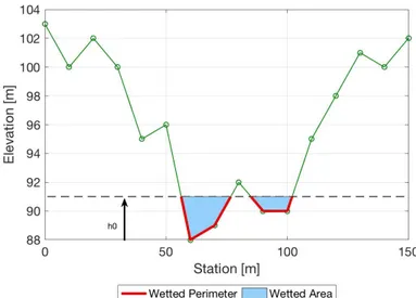
Wetted Area and Perimeter in a Natural Cross-Section In order to determine the variables of the model that are a function of the geometry of the river, including the wetted area A, the wetted perimeter P , the gauge stage h and the width of the upper layer B, a Matlab code has been developed.

To be consistent with the other models, the code has been implemented to fill with water the cross-section in the same way that Hec-Ras does. Hec-Ras considers a constant level and it fills with water all the area between that elevation and the cross-section.

Starting from a known discharge value Q0 and known coordinates of a

specific cross-section, the code follows these steps:

(a) Set of an initial gauge height h0 as first guess, usually set as an

underestimated value. 0.1 m has been chosen.

(b) The code identifies the intersection points between the constant level and the river cross-section starting from the known coor-dinates of the ones that compose the geometry. An example on a random cross-section has been generated to better understand the code’s behavior.

(40)

Figure 9: Example of Matlab code procedure with a random section

(c) It identifies the area under the constant h0 level through a

numer-ical integration (wetted area A) and, consequently, it estimates the wetted perimeter P by the summation of the segment under the elevation h0 that compose the geometry.

(41)

Figure 10: Wetted Area and perimeter

(d) The discharge through the Manning-Strickler formula is com-puted: QM S = 1 nAR 2/3p_S 0 (35)

where n is the Manning coefficient that has been considered unique for all the cross-section for simplicity of the code, A the wetted area, R the hydraulic radius, known as the ratio between the the wetted area and the wetted perimeter A/P and S0 the river slope.

(e) If Q0 = QM S, the Manning-Strickler equation is satisfied. That

means that the initial guess h0 coincides with the real gauge

height. If Q0 > QM S, the code restart from point a) with

an-other guess on the height, set being equal to h + dh, where dh has been being defined equal to 0.05 m.

(42)

Figure 11: Second Iteration of Matlab Code

The code has been validated by applying it on di↵erent cross-section shapes scenarios. The rectangular, triangular and trapezoidal section have been tested for a given value of discharge. The values of wetted area and perimeter obtained from the code matched the ones derived manually from the Manning-Strickler equation. Some results for the rectangular, triangular and trapezoidal sections have been reported. Manning’s roughness coefficient has been set to 0.03, the slope to 0.002 and the discharge to 100 m3_/s.

(43)

(a) Rectangular CS (b) Triangular CS

(c) Trapezoidal CS

Figure 12: Matlab’s code validation on three di↵erent Cross-Sections (CS)

Table 2: Wetted Area and Perimeter obtained through the Matlab code for three di↵erent shapes of cross-section

CS Wetted Area [m2_{] Wetted Perimeter [m]}

Rectangular 39.60 17.92

Triangular 39.44 17.76

(44)

3.2 Hydraulic Model

A hydraulic model is a mathematical model of a water system and is used to analyse the system’s hydraulic behaviour.

The physical laws which govern the flow of water in a river are the conservation of mass and the moment equation. By expressing all the terms involved and rearranging the equations [33], the St. Venant equa-tions are obtained. The two expression that describe the phenomena are: @Q @t @ @s ✓ Q2 A ◆ + gA ✓ @h @s i + ◆ = 0 (36) @Q(s, t) @s + @A(s, t) @t = 0 (37)

where Q is the discharge, A the wetted area, h the hydraulic level, s the spatial coordinate, t the temporal coordinate, i the gravitational e↵ects and the resistance e↵ects.

Being the solution not obtainable analytically, numerical methods are widely used to solve the system equations [40][41]. Commercial software implement di↵erent techniques.

3.2.1 HEC-RAS

Hec-Ras modelling system is a software developed by the Hydrologic Engineeric Center (HEC) of the US Army Corps of Engineers [42]. It allows to perform one-dimensional steady flow, one and two-dimensional unsteady flow calculations, sediment transport/mobile bed computa-tions, and water temperature/water quality modeling. Being the wave propagation a phenomena that varies on space and time, unsteady sim-ulations have been performed in this study. For unsteady conditions the software solves the full St. Venant equations using an implicit finite di↵erence scheme, by means of a solver adapted from the UNET model by Barkau [43].

(45)

3.3 Performance Indexes

Di↵erent performance indexes have been used to assess the performance of a model [44] [45] and the issue about which index is the most truly representative of a quality model has been taken into account by sev-eral authors [46] [47] [48]. The most widely used to assess the accuracy of hydrological models are the Mean Absolute Error (M AE), the Root Mean Square Error (RM SE) and the Nash-Sutlci↵e performance Effi-ciency (N SE) [49]. M AE = N P i=1| ˆ xi xi| N (38) RM SE = v u u u t N P i=1 ( ˆxi xi)2 N (39) N SE = 1 N P i=1 ( ˆxi xi)2 N P i=1 (xi xM)2 (40)

where ˆxi is the computed value at a certain instant of time, xi the

observed value at the same instant of time and xM the mean of the

observed variable. Being the goal of this study the evaluation of the accuracy of di↵erent models on the wave propagation, the variable in discussion is the discharge values that compose the hydrograph. The M AE is indicative of the average magnitude of errors in a series of data, without considering their direction. It’s the average over the test sample of the absolute di↵erences between the computed values and the observed ones where all individual di↵erences have equal weight. The RM SE, instead, is a quadratic scoring rule that also measures the average magnitude of the error. It’s the square root of the average of squared di↵erences between the computed values and actual

(46)

observa-tion.

The N SE is a normalized statistic that determines the relative magni-tude of the residual variance (”noise”) compared to the measured data variance (”information”) [49].

The first two indexes range from zero to infinite, where zero means the perfect reproduction of the observed phenomena, while the third one assumes values between minus infinite and one (pefect reproduction).

Depending on the study case, the M AE and RM SE can assume dif-ferent values that are directly related to the magnitude of the input data. For example, an accurate model representative of an hydrograph with discharge values that vary in the range between 1000 and 3000 m3_{/s could have an higher value of M AE or RM SE if compared to}

a less accurate model of an hydrograph in the range of 50-200 m3_/s.

Therefore, the need to be able to compare the model performance on an absolute scale has led to the use of the N SE as the optimal in-dex performance [50]. This inin-dex takes into account not just the peak discharge, thus the shape of the hydrograph.

3.4 Model Calibration and Validation

3.4.1 Muskingum Model

The three coefficients are function of two parameters, x and k, that have to be calibrated from an observed hydrograph. Muskingum model assumes a linear relationship between channel storage and weighted flow. However, in some cases this hypothesis is not satisfied. There-fore, di↵erent authors proposed several calibration techniques in case of non-linearity [51] [52] [53]. Commonly, to find the couple of optimal parameters, the following passages are followed:

(47)

3.4 Model Calibration and Validation

generic stretch, the following expression is derived:

k = 0.5((I(t + t) + I(t)) (O(t + t) + O(t)))

x(I(t + t) I(t)) + (1 x)(O(t + t) O(t)) (41) • Assuming a value of x as first guess, it is possible to compute the

values of the numerator and denominator of Eq.41.

• By plotting the values of the numerator along the abscissa and the ones of the denominator along the ordinate, a close curve is obtained.

• The value of x that makes the curve as close as possible to the straight line is considered to be the optimal parameter. The in-verse of the slope of that straight line gives k coefficient.

An alternative methodology for model calibration has been found efficient when the range of the parameter was known [54] [55]. It follow these steps:

(a) A combination of the two parameters is chosen.

(b) The model is then run and error or performance indexes are com-puted between the observed hydrograph and the wave propagated in correspondence of the station at the end of the river stretch. (c) points a) and b) are repeated in a loop changing every time the

values of x and k, until the window of possible parameters is covered.

(d) After having obtained a wide number of simulations, a surface representing the error or model performance can be build. (e) The optimal parameters are found as the couple that minimize

(48)

Knowing that the x, known as the wedge storage, varies in the range 0 0.5 [5], a thousand values of this coefficient have been tested. The value of k, the storage-time constant, instead, assumes di↵erent val-ues function of the rapidity of the propagation of the wave. Therefore, being this value range not defined and changing case by case, a wide window of this parameter has been initially tested with a frequency of 1000 seconds. After having found the optimal x and k, the window of the wedge storage has been reduced around the optimal position. Then, the model has been run again with discretization in time every 1 second to find finer results.

Benchmark Case The two di↵erent approaches have been applied on a benchmark case. Observed Inflow and Outflow have been shown in Figure 13. Both of them provided close values of optimal param-eters, that means optimal results in model performance. Being the first methodology dependent on subjective interpretation, such as ”how much the curve is close to a straight line”, the second approach has been used for the calibration procedure of the Muskingum model cal-ibration. Figure 12 shows the results of the calibration obtained with the two procedures.

(49)

(a) Method 1 (b) Method 2

Figure 13: Calibration Procedure Benchmark Case

Table 3: Calibration Parameters from di↵erent approaches Methodology x [-] k [s]

Staight Line 0.151559154 8280 Contour 0.157657658 8300

The outflows derived from the two methodologies have been re-ported in the following figure.

(50)

The performance of the hydrological model has also been tested using all the three indexes cited in Section 4.3. The N SE and RM SE usually lead to the same couple of optimal parameters. The M AE, instead, reaches slight di↵erent results. In according to what specified in Section 4.3, the results obtained using the N SE as performance parameter has been considered as the optimal ones.

This procedure has been repeated for the di↵erent spacing of the cross-sections. Therefore, 48 couple of parameters have been obtained: a pair for the six spacing scenarios, for eight rivers. After having obtained the optimal parameters, the models have been validated on nine di↵erent events.

3.4.2 Muskingum-Cunge-Todini Model

All the expressions in the equations that describe Muskingum-Cunge-Todini model are a function of coefficient with physical meaning and directly dependent on the cross-section geometry, such as the wetted area and the wetted perimeter. Being the Manning’s roughness coef-ficient unknown and, as explained in Section 4.1.3, considered being unique for all the river geometry, a calibration procedure on this pa-rameter has been conducted. Expected values of Manning’s coefficient are in the range between the ones found from the calibration procedure of HEC-RAS model.

Several values for the Manning’s roughness coefficient have been tested. Its range varies from the lowest value of the range for the main channel considered in the HEC-RAS model to the highest value of the flood-plain. The model have been run by varying the parameter by 0.002 s/m1/3 _{and, for each of it, the N SE has been computed between the}

propagated wave and the observed outflow at the control station. The value that has guaranteed the highest model performance has been as-signed to the Manning’s roughness coefficient. The model’s stability

(51)

has been verified by checking at the Courant Number, as explained in Section 4.1.3.

3.4.3 HEC-RAS

Hec-Ras model have been used to simulate the wave propagation along the river stretches, through an unsteady flow analysis. The models have been calibrated by varying Manning’s roughness coefficients: one for the main channel and one for the floodplain. The calibration proce-dure has been carried out similarly to the one used for the Muskingum model, by varying the two coefficient in a certain range. An initial as-sessment of roughness coefficient has been set looking at the physical characteristics of the river. The range of the tested coefficient varies case by case and have been reported in the following table.

Table 4: Range of Manning’s roughness coefficient for each of the study case

River n Channel [s/m1/3_{] n Floodplain [s/m}1/3_]

Apalachicola 0.05-0.11 0.14-0.18 Arkansas 0.015-0.04 0.05-0.13 Brazos 0.02-0.07 0.09-0.15 Connecticut 0.012-0.03 0.05-0.10 Missouri 0.013-0.04 0.05-0.12 Pecos 0.01-0.04 0.04-0.09 Pembina 0.04-0.09 0.10-0.16 Red 0.015-0.04 0.10-0.15

All combinations in this range have been tested, by varying each of the two coefficient by 0.002 s/m1/3_{. For each couple of parameters the}

performance of the model has been assessed by using the N SE on the computed and observed outflow. The pair of Manning’s coefficient with the higher performance index has been considered the optimal one.

(52)

The physical meaning of the Manning coefficient is connected to the roughness characteristics of the river. However, being it the calibra-tion parameter, it also compensates other sources of errors, including the non-satisfactory geometry resolution. Therefore, values obtained from the calibration procedure could also not be truly representative of the only roughness characteristics. Nevertheless, the values that the parameter assumes are still in a range of physical meaning.

(53)

4 Results and Discussions

In this section the results of the calibration and validation procedure on the discharge values are presented. Additionally, the model’s per-formances have been analyzed through boxplots. A final test of the models on the gauge height have been presented.

4.1 Assessing Performance on Flow Data

The calibration procedure has led to the results presented in the fol-lowing figures.

(54)

(55)

4.1 Assessing Performance on Flow Data

(b) Pembina, Brazos, Red and Pecos Rivers Figure 15: Models Calibration

(56)

Table 5: NSE values obtained during the calibration procedure of the Muskingum model for the 6 di↵erent spatial discretization used for the 8 rivers reaches 1km 2km 5km L/3 L/2 L Apalachicola 0.78 0.80 0.84 0.95 0.96 0.94 Arkansas 0.91 0.92 0.92 0.94 0.94 0.87 Brazos 0.81 0.82 0.84 0.88 0.89 0.91 Connecticut 0.98 0.98 0.98 0.98 0.99 0.99 Missouri 0.96 0.96 0.96 0.97 0.97 0.98 Pecos 0.88 0.89 0.90 0.92 0.92 0.89 Pembina 0.90 0.90 0.92 0.95 0.96 0.96 Red 0.91 0.92 0.92 0.96 0.97 0.98

Table 6: NSE values obtained during the calibration procedure of the MCT model for the 6 di↵erent spatial discretization used for the 8 rivers reaches 1km 2km 5km L/3 L/2 L Apalachicola 0.79 0.73 0.73 0.83 0.83 0.88 Arkansas 0.84 0.52 0.76 0.88 0.79 0.76 Brazos 0.81 0.79 0.64 0.85 0.88 0.80 Connecticut 0.93 0.97 0.99 0.97 0.90 0.89 Missouri 0.97 0.97 0.96 0.92 0.96 0.91 Pecos 0.76 0.94 0.68 0.73 0.84 0.86 Pembina 0.87 0.88 0.67 0.78 0.91 0.90 Red 0.95 0.89 0.91 0.92 0.89 0.96

(57)

Table 7: NSE values obtained during the calibration procedure of the HEC-RAS model for the 6 di↵erent spatial discretization used for the 8 rivers reaches 1km 2km 5km L/3 L/2 L Apalachicola 0.95 0.95 0.95 0.97 0.92 0.92 Arkansas 0.89 0.90 0.83 0.92 0.92 0.94 Brazos -0.60 -0.61 0.84 0.90 0.88 0.91 Connecticut 0.97 0.92 0.98 0.98 0.99 0.98 Missouri 0.97 0.97 0.97 0.97 0.97 0.97 Pecos -0.10 -0.68 -0.59 0.72 -0.27 -0.85 Pembina 0.91 0.95 0.94 0.90 0.82 0.96 Red 0.98 0.97 0.97 0.98 0.98 0.94

As observed, the three models appear to provide accurate results, except for the two case studies of Brazos and Pecos river, where Hec-Ras model is not able to propagate the inflow for spacing 2 km and 1 km and for all the cross-sections scenarios, respectively. The cause of this prob-lem is linked to the quality of river geometry, being this model directly influenced by the cross-sections. In fact, by having a look at these two cases, it is noticeable how the river channel is not properly described, due to the small width of the river. In some stretches, the width of these two rivers appears to be less than 30 m, which coincide with the spatial resolution of the Digital Elevation Model used to extrapolate the information about the river geometry. This fact leads to inaccurate cross-sections, in which the main channel is not even represented, or shaped with just one point. Due to this fact, the cross-sections don’t present a certain area characterized by lower elevation (main channel), thus, the volume of water is spread in di↵erent position in each of the cross-section, depending where the area with lower elevation is. The variability in shape in observed cross-sections is very high. So, when the number of cross-sections increases in the river stretch (i.e., from origi-nal L to 1 km), the shape variability also increases. This variable way

(58)

to fill the cross-sections translates in disconnected value of wetted area, perimeter, hydraulic radius and which Manning’s roughness coefficient is involved between a section and a following one. This high variability of inaccurate cross-sections leads to an incorrect wave propagation. In case of lower density of geometry sampling, HEC-RAS interpolates au-tomatically the cross-sections, hence, reducing the variability in shape and, therefore, the wave is propagated properly. This is the case of Bra-zos river in which, for short spacings, HEC-RAS returns wrong results, while, for higher spacings, it is able to propagate the wave properly. To show the geometry inaccuracy and its high variability in shape, three representative cross-sections of Brazos river, spaced by 2 km, have been reported in Figure 16.

(a) Cross-Section at 54 km (b) Cross-Section at 56 km

(c) Cross-Section at 58 km

Figure 16: Cross-Section variability for Brazos river

Because of the two case studies’ inaccurate results, the two rivers have been excluded from the further analysis.

(59)

other eight events can be found in the Appendix.

(60)

(b) Missouri, Pembina and Red Rivers Figure 17: Models Validation

For each of the case studies and for each scenario of cross-section geometry availability nine values of N SE have been obtained. These

(61)

results have been presented through the use of a boxplot. Additionally, to assess in a more generalized way the behaviour of the three models on the di↵erent scenarios, a boxplot combining all the N SE values for each spacing has been done.

(62)

(b) Arkansas River

(63)

(d) Missouri River

(64)

(f) Red River

Figure 18: Model Performances

Muskingum model performs well for all the case studies and for each of the spacings, being this model not influenced by the river geometry. The values of median and the variability range stay approximately con-stant for all the cross-sections scenarios availability until L/2. After this spacing, the median slightly increase and the variability is reduced due to the nature of the model itself. In just one river this trend has not been verified, this is the case of Arkansas river. The reason of this behaviour is directly connected with the event with which the model has been calibrated. This event, in fact, could be a↵ected by lateral inflow from the release of an hydraulic structure and, therefore, could generate lower performance for those events that doesn’t present any inflows. In fact, by looking at the results of the calibration procedure, Muskimgum model, for spacings up to L/2, slightly underestimated the observed outflow. This fact leads to better validation performances if the events are not subjected by any inflows. Instead, for dx = L, Musk-ingum model properly reproduced the observed discharges. Therefore, the validations appear to be overestimated.

(65)

The hydraulic model implemented, HEC-RAS, does not present an overall trend but it varies case by case. In particular, for the case of meandering and braided rivers, identified as classes D and E, the model performance increases with the increasing of the spacing, reach-ing the maximum performance for dx = L. Instead, in more straight and wider rivers (group B and C), the values of median and the vari-ability range do not present big di↵erences for each of the cross-section scenario availability. Similar findings have been presented by Castel-larin et all [18], where the increment of the density of the cross-sections did not lead to considerably higher model performance. By looking at the river geometry of this group of rivers (Arkansas, Connecticut and Missouri), it’s noticeable how the cross-sections are characterized by the presence of a main channel and floodplain area, at an higher eleva-tion. Instead, in rivers with the presence of meanders or lateral pools (Apalachicola, Pecos and Red), the cross-sections present more areas at the same elevation. Sometimes, the level of these lateral pools is lower than the one of the bottom of the main channel (that is the same as the gauge height at the moment of the passage of the satellite). Similarly to the case of Brazos and Pecos river, there is a high variability in shape between following cross-sections. However, the width of these rivers is higher than the spatial resolution of the SRT M and, therefore, a main channel is always shaped in all the cross-sections. Sometimes, the vol-ume of water is not properly distributed in the geometry where it was supposed to be, for the reason of the presence of lower elevation areas. This fact a↵ects the quality of the wave propagation. Nevertheless, the outflows have been computed with satisfactory results for this group of rivers even though the shape of the cross-sections is not optimal. Representative cross-sections for a river with presence of meanders and for a linear one has been reported below.

(66)

Figure 19: Cross-Section for Red river, braided river

(67)

For high spacing, the geometry variability is neglected and the input and output cross-sections are interpolated automatically by HEC-RAS, without generating any non-physical cross-section shape in between. A continuity in the cross-section geometry is achieved and higher perfor-mance of the model are obtained.

Muskingum-Cunge-Todini, instead, gives comparable results with the other two methods in terms of median and variability. Also in this case the river geometry a↵ects the performance of the model, as the case of HEC-RAS. Moreover, the quality of the results are strictly connected with the numerical stability and the explicit approach implemented. These factors mix together arising di↵erent model performance for the six case studies.

For each of the six scenarios of cross-section availability, all the model performance indexes of the six case studies have been grouped. For each spacing, 54 values of N SE compose the following boxplot.

(68)

Performance indexes are overall high: the median values range be-tween 0.85 and 0.95. Hydrologic models present higher median for the spacings up to L/2, while, above that value, Hec-Ras has slight higher median. The variability of the hydraulic model, instead, is higher for all the cross-section geometry scenarios than the hydrologic models. In the speific, Muskingum model’s variability is smaller than the MCT one.

HEC-RAS and Muskingum-Cunge-Todini’s model performance rise, in terms of median and range variability, with the increasing of the spacing among the cross-sections, ie when the higher di↵erences in shape of an inaccurate geometry are neglected. Muskingum model, instead, does not present big variation in the medians but it decrease its variability by considering high spacings, due to the nature of its mathematical approach.

(69)

4.2 Assessing Performance on Water Levels

The water levels obtained with HEC-RAS and Muskingum-Cunge-Todini appear to be underestimated if compared with the observations. Three events for the Missouri, Connecticut and Arkansas river have been re-ported.

(a) Missouri River (b) Connecticut River

(c) Arkansas River

Figure 22: Water Levels for three of the case studies

The reason behind these results is due to the river geometry imple-mented in the models. As previously said, the cross-sections have been extrapolated from the SRT M Digital Elevation Model with spacing resolution of 30 m. In correspondence of the river, the radar detects the elevation of the water level and, consequently, the bathymetry of the river is neglected. The cross-sections have been therefore filled from this elevation rather than the physical bottom of the main chan-nel. The main channel detected by the SRT M has an higher elevation

(70)

and, therefore, it is closer to the floodplain. The volume of water has been then filled firstly in the main channel but, due to its elevation close to the floodplain, it has been also spread laterally. In reality the same amount of water would have been filled from the bottom of the main channel and, eventually, in the floodplain. Due to this laterally expansion rather than the vertical filling in the main channel, the re-sults underestimate the observed gauge height.

The two models applied don’t return the same gauge height due to the fact that MCT has been implemented considering just one value of roughness coefficient rather than the two used in HEC-RAS, one for the main channel and one for the floodplain. More the volume of wa-ter stays inside the main channel, more the wawa-ter levels obtained with HEC-RAS are lower than the ones from MCT. This is due to the fact that Manning’s roughness coefficient of the main channel in HEC-RAS is lower than the unique one implemented in MCT, expected to be a value in between the ones of the main channel and the floodplain. Vice versa, more the floodplain area is involved, more the gauge height of HEC-RAS are higher than the ones obtained from MCT for analogue reasoning.

(71)

5 Conclusions

Hydraulic and hydrologic routing models require a considerable amount of information as input, including the geometry of the river channel. These amount if data could be unknown or hardly reparable though, restraining the applicability of the model itself.

To assess the influence of the river geometry availability on the models performance and verify their applicability in case of limited information about the river geometry, the Muskingum, Muskingum-Cunge-Todini and HEC-RAS models have been applied on eight rivers under di↵erent scenario of equidistant cross-sections availability.

In case of limited information on cross-sections geometry, that means spacing between them higher than L/3, with L the length of the river reach, all the three models show accurate and comparable results. In fact, the median of the N SE, the index used to assess the performance, is higher than 0.9 for all of them. In case of the need to decide the fre-quency of sampling, it is better to avoid dense cross-sections, especially for meandering and braided rivers, because of the non-accurate geome-try that could lead to a less accurate wave propagation. In fact, values of median of the NSE at low spacing among the cross-sections appear to be lower than the one for less dense ones. Moreover, the variability of the performance index decreases by decreasing the density of sampling. The thesis has led to the follow outcomes:

• The morphological conditions, especially the river path, influence the quality of the extrapolated cross-sections from the Digital El-evation Model with 30 m resolution. Due to the fact that with remote sensing techniques it is not possible to observe bathymet-ric data, the main channel could be shaped partially or not even shaped in relation to the stream condition at the moment of the passage of the satellite. Moreover, the variability in shape of

(72)

fol-lowing cross-sections is high for meandering or braided rivers, due to the nature itself. Thus, inaccurate river geometry lead to a less accurate wave propagation. Instead, in more linear rivers there’s always the presence of a well defined main channel, that could have been neglected partially for the conditions of the satellite previously cited, but still with lower elevation than the flood-plain.

• In scarcity condition on the knowledge of cross-section geome-try all the three models reproduce the propagated wave properly. The Muskingum model is the easiest to build, the one with lower computational time and it does not require any input data about the river geometry and its roughness. However, this model, as the other hydrologic routing models, does not provide any infor-mation about the water levels. If in a specific case study gauge heights are needed, they should be obtained through secondary tools or HEC-RAS model should be implemented. Moreover, ob-served data are strictly required for the calibration procedure while, the other two models implemented, could be applied even in absence of observed data, being their coefficient based on phys-ical meaning.

• There are not significant di↵erences on the model performances obtained from dense or sparse cross-sections. Therefore, there’s no need to build the model with short spacing between them. On the contrary, dense frequency of sampling on the river geom-etry cause a decrease on the model performance due to the high variability in shape of a non satisfactory geometry, as previously explained.

When applying a model it is important to have observed data to vali-date the model. In this study, due to the missing data, an event-based

(73)

calibration and validation has been applied. This results in limitation of the applicability of the models, which are usually calibrated both on regime discharges than on peak events. Moreover, all the changes of the ground composition have been neglected, due to the implementation of a unique Manning’s roughness coefficient in MCT and one value for the main channel and one for the floodplain in HEC-RAS.

The cross-sections implemented could not be satisfactory representative of the real shapes, due to their extrapolation from a mid-low spatial resolution of a remote sensing product, which neglect the bathymetry of the river. The source of error of the bad river geometry has been compensate with the choice of the Manning’s parameters, which be-came therefore not just truly representative of the ground roughness. Despite the correct wave propagation, the geometry is still inaccurate for the evaluation of the water levels. Furthermore, in the models, lat-eral inflows have been neglected. This is a choice in accordance to the criteria followed for the river selection. However, in some case studies, lateral inflow is present and it hasn’t been taken into account.

The implemented river geometry has demonstrated to be inaccurate, especially when the cross-sections are taken with a dense frequency, due to the issues related of being a remote sensing product. Future works could concern the influence of the availability on the model perfor-mances with more realistic cross-sections derived from ground surveys or remote sensing products plus the implementation of methods to re-construct the bathymetry of the main channel, not possible to obtain remotely. In this way there could be given an exhaustive influence of geometry availability on hydraulic and hydrologic routing models with more reliable cross-sections. The implementation of mathematical methods for the main channel reproduction on freely-downloadable re-mote sensing products could then became a valid alternative to ground

(74)

(75)

REFERENCES

References

[1] H. Winsemius and P. Ward, “Aqueduct global flood risk coun-try rankings,” World Resources Institute: Washington, DC, USA, 2015.

[2] P. C. D. Milly, R. T. Wetherald, K. Dunne, and T. L. Delworth, “Increasing risk of great floods in a changing climate,” Nature, vol. 415, no. 6871, pp. 514–517, 2002.

[3] M. H. Tewolde and J. Smithers, “Flood routing in ungauged catch-ments using muskingum methods,” Water SA, vol. 32, no. 3, pp. 379–388, 2006.

[4] G. T. McCarthy, “The unit hydrograph and flood routing,” in proceedings of Conference of North Atlantic Division, US Army Corps of Engineers, 1938, 1938, pp. 608–609.

[5] J. Cunge, “On the subject of a flood propagation method (musk-ingum method), j. hydraulics research,” International Association of Hydraulics Research, 1969.

[6] E. Todini, “A mass conservative and water storage consistent vari-able parameter muskingum-cunge approach,” Hydrology and Earth System Sciences Discussions, vol. 4, no. 3, pp. 1549–1592, 2007. [7] P. Choudhury, R. K. Shrivastava, and S. M. Narulkar, “Flood

rout-ing in river networks usrout-ing equivalent muskrout-ingum inflow,” Journal of Hydrologic Engineering, vol. 7, no. 6, pp. 413–419, 2002.

[8] H. Lee, Y. Liu, M. He, J. Demargne, and D.-J. Seo, “Variational assimilation of streamflow into three-parameter muskingum rout-ing model for improved operational river flow forecastrout-ing,” The EGU General Assembly, 2011.

(76)

[9] F. Hicks and T. Peacock, “Suitability of hec-ras for flood forecast-ing,” Canadian water resources journal, vol. 30, no. 2, pp. 159–174, 2005.

[10] J. E. Hilland, F. V. Stuhr, A. Freeman, D. Imel, Y. Shen, R. L. Jordan, and E. R. Caro, “Future nasa spaceborne sar missions,” IEEE aerospace and electronic systems magazine, vol. 13, no. 11, pp. 9–16, 1998.

[11] J. J. Van Zyl, “The shuttle radar topography mission (srtm): a breakthrough in remote sensing of topography,” Acta Astronau-tica, vol. 48, no. 5-12, pp. 559–565, 2001.

[12] K. Yan, G. Di Baldassarre, and D. P. Solomatine, “Exploring the potential of srtm topographic data for flood inundation modelling under uncertainty,” Journal of hydroinformatics, vol. 15, no. 3, pp. 849–861, 2013.

[13] G. Di Baldassarre, G. Schumann, and P. D. Bates, “A technique for the calibration of hydraulic models using uncertain satellite observations of flood extent,” Journal of Hydrology, vol. 367, no. 3-4, pp. 276–282, 2009.

[14] A. M. Ali, D. Solomatine, and G. Di Baldassarre, “Assessing the impact of di↵erent sources of topographic data on 1-d hydraulic modelling of floods,” Hydrology and Earth System Sciences, vol. 19, no. 1, pp. 631–643, 2015.

[15] M. Wood, J. Neal, P. Bates et al., “Calibration of channel depth and friction parameters in the lisflood-fp hydraulic model using medium resolution sar data and identifiability techniques,” Hy-drology and Earth System Sciences, vol. 20, no. 12, pp. 4983–4997, 2016.

(77)

REFERENCES

[16] E. H. Altenau, T. M. Pavelsky, P. D. Bates, and J. C. Neal, “The e↵ects of spatial resolution and dimensionality on modeling regional-scale hydraulics in a multichannel river,” Water Resources Research, vol. 53, no. 2, pp. 1683–1701, 2017.

[17] K. Yan, A. Tarpanelli, G. Balint, T. Moramarco, and G. D. Baldassarre, “Exploring the potential of srtm topography and radar altimetry to support flood propagation modeling: Danube case study,” Journal of Hydrologic Engineering, vol. 20, no. 2, p. 04014048, 2015.

[18] A. Castellarin, G. Di Baldassarre, P. D. Bates, and A. Brath, “Op-timal cross-sectional spacing in preissmann scheme 1d hydrody-namic models,” Journal of Hydraulic Engineering, vol. 135, no. 2, pp. 96–105, 2009.

[19] M. H. Naghshine, F. F. Raof, and A. Khoshrftar, “The study of flood hydraulics before the building of maroon dam by hec-ras, maskingam and muskingum-cunge method,” 2013.

[20] M. G. Wolman and L. B. Leopold, “River flood plains: some ob-servations on their formation,” 1957.

[21] E. W. Lane, “Study of the shape of channels formed by natural streams flowing in erodible material, a,” MRD sediment series; no. 9, 1957.

[22] D. Culbertson, L. Young, and J. Brice, “Scour and fill in alluvial channels with particular reference to bridge sites,” US Dept. of the Interior, Geological Survey,, Tech. Rep., 1967.

[23] D. L. Rosgen, “A classification of natural rivers,” Catena, vol. 22, no. 3, pp. 169–199, 1994.

(78)

[24] USGS, “Usgs streamgaging network.” [Online]. Avail-able: https://www.usgs.gov/mission-areas/water-resources/ science/usgs-streamgaging-network?qt-science center objects=0# qt-science center objects

[25] J. Reynolds, S. Halldin, J. Seibert, C.-Y. Xu, and T. Grabs, “Robustness of flood-model calibration using single and multiple events,” Hydrological Sciences Journal, pp. 1–12, 2019.

[26] Z. Kalantari, S. W. Lyon, P.-E. Jansson, J. Stolte, H. K. French, L. Folkeson, and M. Sassner, “Modeller subjectivity and calibra-tion impacts on hydrological model applicacalibra-tions: An event-based comparison for a road-adjacent catchment in south-east norway,” Science of the Total Environment, vol. 502, pp. 315–329, 2015. [27] S. K. Singh and A. B´ardossy, “Calibration of hydrological models

on hydrologically unusual events,” Advances in Water Resources, vol. 38, pp. 81–91, 2012.

[28] C. T. Ackerman, “Hec-georas–gis tools for support of hec-ras using arcgis, user’s manual,” US Army Corps of Engineers–Hydrologic Engineering Center (HEC), vol. 4, 2009.

[29] V. M. Ponce and V. Yevjevich, “Muskingum-cunge method with variable parameters,” Journal of the Hydraulics Division, vol. 104, no. 12, pp. 1663–1667, 1978.

[30] A. D. Koussis, “Comparison of muskingum method di↵erence schemes,” Journal of the Hydraulics Division, vol. 106, no. 5, pp. 925–929, 1980.

[31] P. E. Weinmann and E. M. Laurenson, “Approximate flood routing methods: a review,” Journal of the Hydraulics Division, vol. 105, no. 12, pp. 1521–1536, 1979.

(79)

REFERENCES

[32] A. A. Smith, “A generalized approach to kinematic flood routing,” Journal of Hydrology, vol. 45, no. 1-2, pp. 71–89, 1980.

[33] F. M. Henderson, “Open channel flow,” New York, Tech. Rep., 1966.

[34] V. M. Ponce and P. Changanti, “Variable-parameter muskingum-cunge method revisited,” Journal of Hydrology, vol. 162, no. 3-4, pp. 433–439, 1994.

[35] X. Tang, D. W. Knight, and P. G. Samuels, “Variable parameter muskingum-cunge method for flood routing in a compound chan-nel,” Journal of hydraulic research, vol. 37, no. 5, pp. 591–614, 1999.

[36] M. G. Ferrick, J. Bilmes, and S. E. Long, “Modeling rapidly varied flow in tailwaters,” Water Resources Research, vol. 20, no. 2, pp. 271–289, 1984.

[37] W. Viessman Jr and G. L. Lewis, Introduction to Hydrology. Up-per Saddle River, NJ: Aprentice Hall.

[38] V. M. Ponce and P. J. Porras, “E↵ect of cross-sectional shape on free-surface instability,” Journal of Hydraulic Engineering, vol. 121, no. 4, pp. 376–380, 1995.

[39] M. Perumal and K. G. R. Raju, “Field applications of a variable-parameter muskingum method,” Journal of Hydrologic Engineer-ing, vol. 6, no. 3, pp. 196–207, 2001.

[40] T. Strelko↵, “Numerical solution of saint-venant equations,” Jour-nal of the Hydraulics division, vol. 96, no. 1, pp. 223–252, 1970.