POLITECNICO DI MILANO
DEPARTMENT OF MECHANICS
Master of Science in Mechanical Engineering
AA 2019-2020
A Restarted Iterated Pareto Greedy
algorithm for the multi-objective
hybrid flow shop scheduling
problem
Candidate: Michele Tota Mat. 859389 Supervisor: Dott. Chunlong Yu Tutor:To my parents, that always gave me strength and support.
Table of contents:
1. Introduction...10
2. Problem description...15
2.1 The hybrid flow shop: problem description and notation………..…16
3. Literature review……….21
3.1 Methods for HFS scheduling problem...22
3.2 Sequence-dependent setup time and unrelated parallel machines…26 3.3 Multi-objective Hybrid Flow hop……….28
3.3.1 The Scheduling problem with Total Tardiness (TT) objective…………...……….30
3.3.2 The scheduling problem with Total Setup Time (TST) objective……….31
3.4 The Restarted Iterated Pareto Greedy Algorithm (RIPG)………...32
4. Methodology……….35
4.1 A model for the SDST hybrid flow shop………36
4.2 Encoding methods………..37
4.3 Decoding methods……….39
4.4 The Restarted Iterated Pareto Greedy……….44
4.4.1 The initialization phase………....46
4.4.2 The selection phase………...48
4.4.4 The Local Search phase………..………..…..51
4.4.5 The restart phase………..…………..……53
5. Numerical results……….……..55
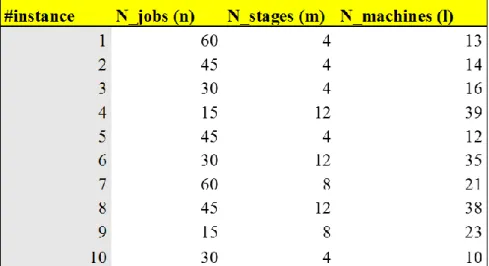
5.1 Benchmark description……….………….………….56
5.2 RIPG calibration……….…………..57
5.3 Performance comparison with NGSAII………..………..66
6. Conclusions……….………..……… 87
7. References………..………..……… 90
8. Appendix……….……….105
8.1 Pseudocode of Initialization phase……….…....106
8.2 Pseudocode of MCDA……….………...107
8.3 Pseudocode of Greedy phase……….…….…..108
8.4 Pseudocode o Local search………...…..…108
List of Figures:
Figure 1- The Hybrid Flowshop ... 18
Figure 2 -Methods classification ... 25
Figure 3- Constraints for HFS ... 28
Figure 4- Objectives for HFS ... 32
Figure 5- Scheduling example ... 37
Figure 6- Encoding/decoding classifications ... 38
Figure 7 - RIPG scheme ... 46
Figure 8 - Initialization procedure scheme ... 48
Figure 9- Hypervolume indicator ... 60
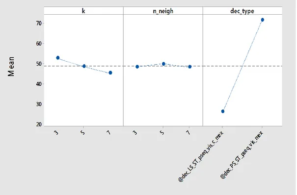
Figure 10- Main effect plot of calibration ... 61
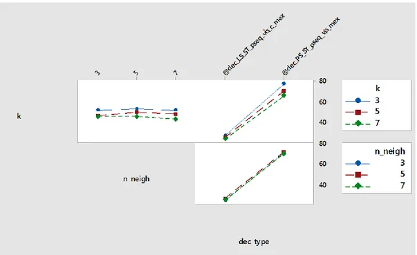
Figure 11- Interaction plot ... 62
Figure 12- Test for equal variances... 64
Figure 13- Normality test ... 64
Figure 14- Scatterplot interval for SRES ... 65
Figure 15 - Tests for comparison ... 67
Figure 16 – Fronts comparison...72
Figure 17- HV means comparison 20 jobs 5 stages...72
Figure 18- HV means comparison 20 jobs 10 stages ... 73
Figure 19- HV means comparison 20 jobs 20 stages ... 73
Figure 20- HV means comparison 50 jobs 5 stages ... 74
Figure 21- HV means comparison 50 jobs 10 stages ... 74
Figure 23 - HV means comparison 100 jobs 5 stages ... 75
Figure 24- HV means comparison 100 jobs 10 stages ... 76
Figure 25- HV means comparison 100 jobs 20 stages ... 76
Figure 26- Standard deviation comparsion 20 jobs 5 stages... 77
Figure 27- Standard deviation comparsion 20 jobs 10 stages... 77
Figure 28- Standard deviation comparsion 20 jobs 20 stages... 78
Figure 29- Standard deviation comparsion 50 jobs 5 stages... 78
Figure 30 - Standard deviation comparsion 50 jobs 10 stages... 79
Figure 31- Standard deviation comparsion 50 jobs 20 stages... 79
Figure 32 - Standard deviation comparsion 100 jobs 5 stages... 80
Figure 33 - Standard deviation comparsion 100 jobs 10 stages... 80
Figure 34- Standard deviation comparsion 100 jobs 20 stages... 81
Figure 35- Main effect plot for comparsion... 82
Figure 36- Interaction plot for comparison ... 82
Figure 37- Scatterplot SRES for comparison ... 84
Figure 38- Normality test for comparison ... 84
List of Tables:
Table 1- Notation ... 20
Table 2 - methods for HFS ... 25
Table 3 - Processing times ecample ... 36
Table 4 - Processing times example ... 36
Table 5 – Resume table per paper ... 41
Table 6 - Notation ... 41
Table 7 - benchmark description ... 56
Table 8 - ANOVA of calibration ... 63
Table 9 - Tukey test ... 66
Table 10 - ANOVA for comparison ... 83
The scheduling of flow shops with multiple parallel machines per stage, which is usually referred to as the hybrid flow shop (HFS), is a complex combinatorial optimization problem encountered in many real-world applications. The problem is to determine the allocation of jobs to the parallel machines as well as the sequence of the jobs assigned to each machine, so as to create a Gantt chart to guide the production activities. The basic HFS scheduling problem has been thoroughly studied in recent decades, both from single objective as well as from multi-objective perspectives, but to the best of our knowledge, little has been done to the multi-objective scheduling problem considering the reduction of total machine setup time as one of the objectives. Given that the machine setups act as non-value-added activities which should be avoided or mitigated from the manufacturing practices, it is important to make a proper schedule which results in short total setup time together with other performance indicators, such as productivity and on-time product delivery. For this reason, this thesis focuses on the HFS scheduling problem with the total tardiness and total setup time objectives. In this work, a simple, yet powerful algorithm for the sequence dependent setup time hybrid flow shop problem is proposed. The presented method, known as Restarted Iterated Pareto Greedy or RIPG, is compared to the NGSA-II, which is a well-known algorithm for multi-objective optimization in literature. Computational and statistical analyses demonstrate that the proposed RIPG method outperforms the NGSA-II in the test instances. We conclude that the proposed method is a candidate to be the state-of-art method for this important and practical scheduling problem.
Chapter 1
11 Production scheduling is one of the most complex activities in the management of production systems. It is closely connected with the firm's performance in terms of speed, reliability, flexibility, quality, and cost. The theory of production scheduling, that aims to provide guidelines and methods, for efficient use of resources, has been the subject of countless papers, over the past five decades. Although several features of scheduling problems are still underexplored due to the variety of production environments, the available resources, restrictions may be imposed and there are multiple objectives to be achieved. Moreover, production scheduling is one of the activities of the Planning, Programming and Production Control. It is responsible for deciding the allocation of resources (machines) over time to perform individual items (jobs and/or batch of jobs), in order to better meet a predefined set of criteria. One can understand the production scheduling as a set of functions of decision-making, involving:
how to allocate jobs on machines over time, called schedule;
decisions about how to order the jobs on a given machine called sequence,
The scheduling of flow shops with multiple parallel machines per stage, usually referred to as the Hybrid Flow Shop (HFS), is a complex combinatorial problem encountered in many real world applications. Given its importance and complexity, the HFS problem has been intensively studied [1]. Hybrid flow shops are common manufacturing environments in which a set of n jobs are to be processed in a series of m stages optimizing a given objective function. There are a number of variants, all of which have most of the following characteristics in common:
The number of processing stages m is at least 2.
Each stage k has machines in parallel and at least IN one of the stages.
12
All jobs are processed following the same production flow: stage 1, stage 2, …, stage m. A job might skip any number of stages provided it is processed in at least one of them.
Each job j requires a processing time p in stage k. We shall refer to the processing of job j in stage k as “operation”.
In the “standard” form of the HFS problem all jobs and machines are available at time zero, machines at a given stage are identical, any machine can process only one operation at a time and any job can be processed by only one machine at a time; preemption is not allowed, the capacity of buffers between stages is unlimited and problem data is deterministic and known in advance. Although most of the problems described in this review do not fully comply with these assumptions, they mostly differ in two or three aspects only; the standard problem will serve as a “template” to which assumptions and constraints will be added or removed to describe different HFS variants. In particular, in specific case, to better represent the reality of many real industrial cases, a sequence dependent setup time will be considered with also unrelated parallel machines and a constraint of machine eligibility. The first limitation of unrelated machines indicates that the parallel machines in a stage are not identical but there could be differences in terms of processing speed or manufacturing technologies applied. These two limitations are very common in many industrial cases and are also less considered in the previous literature HFS scheduling problem. In terms of the objective, most researches focus on minimizing the makespan of a schedule. However, in most of the cases, makespan is not the most important criterion to considered. Like in the make-to-order environment, job tardiness should be given higher priority than makespan. Also, the setup times/costs [2] are considered as another important indicator to evaluate the schedule quality, but seldom considered in the literature. These motivate us to consider the total tardiness and total setup time as objective functions to be minimized.
13 The scheduling problem can be denoted using a triplet α|β|γ notation where, α defines the shop configuration, β describes the constraints and assumptions and γ indicates the objective function. Consequently, the described scheduling problem is denoted as:
𝐹𝐻𝑚, ((𝑅𝑀𝑘) 𝑘=1
𝑚 )| 𝑀
𝑗, 𝑆𝑠𝑑| ∑𝑇𝑗, 𝑇𝑆𝑇
Here, 𝐹𝐻𝑚 indicates a HFS with m stages; ((𝑅𝑀𝑘)𝑘=1𝑚 ) represents that each stage consists of multiple unrelated machines; Mj represents machine eligibility; ∑ 𝑇𝑗 indicates the total tardiness objective and TST for the total setup time.
Hybrid flow shop scheduling problem is a discrete optimization problem. When multi-objectives are to be optimized, typical multi-objective optimization methods like NSGA-II [3], SPEA2 [4] can be applied. Yet, other algorithms exist, and in particular one potential competitor is the Iterated-greedy search [5]. It has been applied to the single-objective flow shop problem [6], multi-objective flow shop problem [7] and obtained state-of-art results. The HFS scheduling problem, in most cases, are NP-hard. For instance, HFS restricted to two processing stages, even in the case when one stage contains two machines and the other one a single machine, is NP-hard, after the results of [8]. Similarly, the HFS when preemption is allowed results also in strongly NP-hard problems, according to [9]. Moreover, the special case where there is a single machine per stage, known as the flow shop, and the case where there is a single stage with several parallel machines, known as the parallel machines environment, are also NP-hard, [10]. However, with some special properties and precedence relationships, the problem might be solvable in polynomial time[11].
The HFS scheduling problem has attracted a lot of attentions given its complexity and practical relevance. HFS is found in all kinds of real world scenarios including the electronics [12], [13], [14], [15], paper [16] and textile,
14 [17], industries. Examples are also found in the production of concrete, [18], the manufacturing of photographic film, [19], [20], and others, [21], [22], [23], [24], [25], [26], [27]. We also find examples in non-manufacturing areas like civil engineering [28], internet service architectures [29] and container handling systems [30] [31]. The results, of this research, may be useful for future research, towards the development of new solution methods, and/or for the application of methods investigated in the context of real companies, with this kind of scheduling problem.
The thesis is organized as follows. Chapter 2 conducts a literature review on exact, heuristic and metaheuristic methods that have been proposed over the last decades, also provides a discussion on different methodologies used to solve the problem and their basic features and components. It explains the terminology used to refer to the different assumptions, constraints and objective functions where reviewed papers are briefly commented and only the most important facts are highlighted. Then, the aim is to focus on applying the optimization method called Restarted Iterated Pareto Greedy (RIPG), which is described and presented in Chapter 3. Chapter 4 discusses the obtained results of the experimental campaign. A comparison between the proposed method and the conventional method is described in Chapter 5. The results may be useful for future research, towards the development of new solution methods, and/or for the application of methods investigated in the context of real companies, with this kind of scheduling problem. These aspects with relative research opportunities in HFS scheduling problem concludes the thesis.
15
Chapter 2
16 This chapter defines the research problem. Furthermore, this chapter presents some considerations about the limitations emerged from the state-of-the-art analysis. The literature review can be organized in three parts. First, we review different methods solving the HFS scheduling problem, which can be categorized by exact, heuristic and metaheuristic methods, considering the most common assumptions and objectives. Then we review papers and organize them according to different criteria. In particular the criteria considered for the classification were, the encoding and decoding procedure used in the algorithms, the machine selection rule adopted in each stage, the technique used, the adopted constraints on the production chain and the considered objectives.
2.1 The Hybrid Flow Shop: problem description and notation
A Hybrid Flow Shop (HFS) consists of series of production stages, each of which has several machines operating in parallel. Some stages may have only one machine, but at least one stage must have multiple machines. The flow of jobs through the shop is unidirectional. Each job is processed by one machine in each stage and it must go through one or more stage [49]. Depending on the adopted assumptions, machines in each stage can be considered identical, uniform or unrelated. When pij = pj/si where pj is the processing time of
job j and si is the speed of machine i, then the machines are called uniform. If
the pijs are arbitrary then the machines are called unrelated. And both of the
uniform and unrelated cases belong to non-identical parallel-machine schedules. In our case, as we already mentioned, there are some differences between them which makes the hypothesis of unrelated parallel machines an important assumption close to the real industrial environment. In fact, HFS is often found in the electronic manufacturing environment such as IC packaging and PCB fabrication, where this assumption is often verified. The
17
dependent. The SDST/HFS problem can be described as follows. A set of n jobs
J = {1, 2, ..., n} have to be processed through m production stages {1, 2, ..., m} following the same production route, i.e., first at stage 1, then at stage 2, and so on until last stage m. Each stage k, k = 1, 2, ..., m, has a set of almost identical parallel machines, Mk (|Mk| ≥ 2 for at least one stage, where | • | denotes the cardinality of a set). Each job j ∈ J can be processed on one of the |Mk| depending on a machine eligibility criterion. We denote the processing time of job j ∈ J at stage k as pk, j. We have a SDST, denoted as sk,j',j, when job j ∈ J is processed immediately after job j' ∈ J (j' ≠ j) on the same machine at stage k. If job j ∈ J is the first job processed on a machine at stage k, its setup time is denoted as sk,j,j. At any time, no job can be processed on more than one machine, and no machine can process more than one job. All jobs are independent and available for processing at time 0. The objective is then to find a schedule so that the Total Setup Time and the Total Tardiness are minimized.
The SDST assumption comes from the need to have a more realistic model of the HFS. Another important mark to be made, is the constraint of machine eligibility which gives a criteria on which machine is eligible to process an operation of a given jobs. The two objectives are to minimize are the total job tardiness and the total setup time.
18 The resume of what stated plus its notation is presented as follows:
In stage i, there are mi unrelated parallel machines with different processing abilities, where mi ⩾ 1.
Between the stages i and i + 1, the buffer capacity is assumed infinite.
Each job consists of a sequence of operations Oi,j where Oi,j denotes the ith operation of job j, which should be carried out on a selected machine in stage
i;
When a job arrives at a stage i, it can select exactly one machine from mi available unrelated parallel machines. The selection is made according to an eligibility index;
After a job is completed at stage i, it may be processed as follows:
1) the job will be immediately delivered to the subsequent stage when one of the machines at stage i + 1 is available;
2) in cases in which there is no available machine at stage i + 1, the job will be stored in the following buffer given the infinite buffer space;
Each machine in the same stage can process only one job at a time, and each job can be executed by only one machine at a time;
19
Preemption is not allowed; that is, a job cannot be interrupted before the completion of its current operation;
Setup times are sequence dependent and all the problem data are deterministic and known in advance;
Machines are reliable and no machine failures can happen.
The following table resumes the adopted notation:
Notation Description
n number of jobs (j =1,…,n)
m Number of stages (i =1,…,m)
k Index for machines inside a stage
pi,j,k Processing time of job j at stage i on machine k
Oi,j,k Operation of job j at stage i on machine k
Ei Set of eligible machines at stage i
Ci,j Completion time of Oi,j,k
dj Due date for job j
si,j Sequence-dependent setup time from job j at stage i.
Tj Tardiness of job j. 𝑇𝑗 = max (0, 𝐶𝑗 − 𝑑𝑗)
T Total Tardiness: 𝑇 = ∑𝑛𝑗=1𝑇𝑗
20 The scheduling problem can be denoted using a triplet α|β|γ notation. In this notation, α defines the shop configuration, β describes the constraints and assumptions and γ indicates the objective functions. Consequently, the described scheduling problem is denoted as:
𝐹𝐻𝑚 ,((𝑅𝑀(𝑘))𝑖=1 𝑚
) |𝑀𝑗, 𝑆𝑠𝑑| ∑ 𝑇𝑗, 𝑇𝑆𝑇
Here, 𝐹𝐻𝑚 , indicates a HFS with m stages; represents that each stage consists of multiple unrelated machines; 𝑀𝑗represents machine eligibility; ∑ 𝑇𝑗, 𝑇𝑆𝑇 indicates the total tardiness and the total setup time objective.
21
Chapter 3
22 3.1 Methods for HFS scheduling problem
In literature, methods for HFS scheduling problem can be categorized as exact and heuristic. Exact methods, including mathematical programming and
branch & bound, solve the problem to find an optimal solution. Although the
branch and bound was first suggested by [67], the first complete algorithm introduced as a multi-objective branch and bound that we identified was proposed by [68]. Based on the “divide to conquer” idea, it consists in an implicit enumeration principle, viewed as a tree search. The feasible set of the problem to optimize is iteratively partitioned to form sub-problems of the original one. Each sub-problem is evaluated to obtain a lower bound on the sub-problem objective value. The lower bounds on sub-problem objective values are used to construct a proof of optimality without exhaustive search. Uninteresting and infeasible problems are pruned, promising sub-problems are selected and instantiated [46]. However, due to the lack of efficient lower bounds, branch & bound approach is limited to simple shop configurations; also, exact methods require long time for solving large instances. Both facts limit the industrial application of exact methods. A practical idea is to search for quasi-optimal solution in a reasonable time. For this reason, the trend of solving HFS scheduling problems with heuristic, especially metaheuristic, is increasing [41]. In the past decade, genetic algorithm (GA) has gained the widest applications. Genetic Algorithms were introduced by Holland [32] and they have been used in many scheduling problems (see for instance [33], [34]). The GA starts with an initial population of possible solutions called chromosomes to the problem. The relative quality of these chromosomes is determined using a fitness function. This quality is used to determine whether the chromosomes will be used in producing the next generation of chromosomes. The next generation is generally formed via the processes of crossover and mutation. Crossover is the process of combining elements of two chromosomes, whereas mutation means randomly altering elements of a chromosome [35]. Among the metaheuristic methods we can underline different ones such as population learning
23
algorithm [37], taboo search [38] and ant colony system [39]. In particular,
the tabu search algorithm TSNS is commonly considered as the most effective solution method for the considered HFS scheduling problem with related parallel machines. Its high efficiency is obtained due to so called reduced
neighborhood based on the block properties and the accelerator designed for Cmax computation for all neighbors of the base solution [42]. A detailed description of all TSNS components can be found in [43]. All these focus on minimizing the makespan but it is not the only scheduling problem tackled; [40] focused on minimizing the weighted completion time in proportional flow shops. Also Hybrid heuristic are used. Memetic algorithms for example are hybrid evolutionary algorithms that combine global and local search by using an evolutionary algorithm to perform exploration while the local search method performs exploitation [36]. There exist hybrid heuristic algorithms that combine particle swarm optimization (PSO) [44] [45] with simulated
annealing (SA) and PSO with tabu search (TS), for example. Particle swarm
optimization is similar to the genetic algorithm technique for optimization in that rather than concentrating on a single individual implementation, a population of individuals (a “swarm”) is considered instead. The algorithm then, rather than moving a single individual around, will move the population around looking for a potential solution. Each individual in the swarm has a position and velocity defined, the algorithm looks at each case to establish the best outcome using the current swarm, and then the whole swarm moves to the new relative location [47]. Instead, Simulated Annealing (SA), introduced in [51], was conceived for combinatorial problems, but can easily be used for continuous problems as well. SA starts with a random solution xc and creates a new solution xn by adding a small perturbation to xc. If the new solution is better than the current one, it is accepted and replaces xc. In case xn is worse, SA does not reject it right away, but applies a stochastic acceptance criterion, thus there is still a chance that the new solution will be accepted, albeit only with a certain probability. This probability is a decreasing function of both the order of magnitude of the deterioration and the time the algorithm has
24 already run. This time factor is controlled by the temperature parameter T which is reduced over time; hence, impairments in the objective function become less likely to be accepted and, eventually, SA turns into standard local search. The algorithm stops after a predefined number of iterations Rmax[48]. Experimental results reveal that these memetic techniques can effectively produce improved solutions over conventional methods with faster convergence [36]. Besides these, in recent years, other less used metaheuristics were proposed for HFS. For example immune evolutionary
algorithm [52] and artificial bee colony [53],[54]. Lastly there have been
presented apply new metaheuristics like water flow-like algorithm [55],
firefly algorithm [57], cuckoo search algorithm [56] to solve HFS problems.
Indeed, different metaheuristics represent different search patterns in the solution space. However, due to the existence of the No-Free Lunch (NFL) Theorem [58], it is more important on how to make use of problem structure information to improve the search procedure than just applying new general purpose optimization methods to HFS problems [41]. Although there exist many different approaches, in last years an important contribution has been given by the Iterated-greedy algorithm. A resume table is presented here.
25 Tabella 2 - methods for HFS
Year Authors Tipology
1960 H. Land, A & G. Doig Branch & Bound
1975 H. Holland Genetic Algorithm
1983 G. Kiziltan, E. Yucaoglu Branch & Bound
1995 J. Kennedy, R. Eberhart Particle swarm optimization
1998 Y. Shi, R.C. Eberhart Simulated annealing
2003 J. Jdrzêjowicz, P. Jdrzêjowicz Population learning algorithm
2004 C. Oðuz, Y. Zinder et al. Taboo search
2005 C. Oguz, M.Ercan Genetic Algorithm
2006 K.C. Ying, S.W. Lin Ant colony system
2006 M. Zandieh, S.M.T.F. Ghomi, S.M.M. Husseini Immune evolutionary algorithm 2011 F. Choong, S. Phon-Amnuaisuk, M.Y. Alias Memetic algorithms
2012 F. Pargar, M. Zandieh Water flow-like algorithm
2013 M.Ciavotta, Minella, Ruiz Iterated greedy algorithm
2014 M.K. Marichelvam, T. Prabaharan, X.S. Yang Firefly algorithm 2014 M.K. Marichelvam, T. Prabaharan, X.S. Yang Cuckoo search algorithm
2015 Z. Cui, X. Gu Artificial bee colony
2016 ] J. Li, Q. Pan, P. Duan Artificial bee colony
Figura 2 -Methods classification
Algorithms
Exact
Branch & Bounf Dynamic programming Lagrangian & surrogate relaxaion methods Implicit enumeration techniquesHeuristic
Greedy Relaxation based Transformation heuristicMeta
heuristic
Simulated annealing Neural networks Tabu search Genetic algorithm26 3.2 Sequence-dependent setup time and unrelated parallel
machines
Unrelated parallel machine scheduling is widely applied in manufacturing
environments such as the drilling operations for printed circuit board fabrication [113] [114] and the dicing operations for semiconductor wafer manufacturing [115]. A lot of papers about HFS have been published in the literature but only a relatively minor fraction of them consider sequence dependent setup times. In the literature, there are three types of parallel
machines scheduling even though most of researches are limited to situations
in which the processing times are the same across all machines. This type is called identical parallel machines (Pm). In the second type, machines have different speed but each machine works at a consistent rate, Qm [116] [117]. Finally, when machines are capable of working at different rates and when different jobs could be processed on a given machine at different rates, the environment is said to have unrelated parallel machines, Rm [116]. Developed algorithms to schedule unrelated parallel machines are capable of generating good solutions when applied to all kinds of parallel machine problems and that’s why they are important. [118] pointed out that unrelated parallel machine problems remain relatively unstudied and presented a survey of algorithms for single-and multi-objective unrelated parallel machine deterministic scheduling problems. There is much research work considering parallel machines, but few unrelated parallel machines or sequence-dependent set-up times (SDST). In general, such a problem is composed of job allocation and job sequencing onto the machines, simultaneously, with similar but not necessarily identical capabilities. In [66] the makespan and total weighted tardiness are optimized simultaneously with a multi-phase genetic algorithm for searching Pareto optimal solutions of a hybrid flow shop group scheduling problem. [69] uses tabu search procedure to address a sequence-dependent group scheduling problem on a set of unrelated-parallel machines where the run time of each job differs on different machines. [70] proposes a new multi-objective approach for solving a no-wait k-stage flexible flow shop scheduling problem to minimize makespan and mean tardiness. Sequence-dependent setup times
27 are treated in this problem as one of the prominent practical assumptions. [71] investigates a bi-objective HFS problem with sequence dependent setup time for the minimization of the total weighted tardiness and the total setup time. To efficiently solve this problem, a Pareto-based adaptive bi-objective variable neighborhood search (PABOVNS) is developed and a job sequence based decoding procedure is presented to obtain the corresponding complete schedule. [72] paper presents an enhanced migrating bird optimization (MBO) algorithm and a new heuristic for solving a scheduling problem. The proposed approaches are applied to a permutation flow shop with sequence dependent setup times. Using an adapted neighborhood, a tabu list, a restart mechanism and an original process for selecting a new leader the MBO’s behavior is improved and it gave state-of-the-art results when compared with other algorithms reference. [73] proposed a genetic algorithm and a memetic algorithm for the F/Sijk, prmu/Cmax [74] introduced an algorithm formed by a new heuristic and a local search improvement scheme for the combined objective of total weighted flow-time and tardiness. [75] offers a comprehensive review of scheduling research with setup times. From an industrial point of view, [119] solve a parallel machine scheduling problem inspired in an aluminium foundry considering objectives related to the metal flow; [120] consider a problem related to multi-product metal foundries; or more recently, [121] tackle, in a metal packaging industry, an unrelated parallel machines scheduling problem with job splitting and sequence-dependent setup times, [122] considers a problem identified in a shipyard modelled by unrelated parallel machines with jobs release dates, precedence constraints and sequence-dependent setup times where machines are eligible, and finally [123] considers a dynamic scheduling problem based on the features of parallel heat treatment furnaces of a manufacturing company. To the best of our knowledge, the problem under consideration has not been addressed in the literature, although some papers address the unrelated parallel machines problem with machine eligibility and setup times with additional constraints.
28 3.3 Multi-objective hybrid Flow Shop
There are several different approaches to the multi-objective optimization. The most immediate and commonly employed methodology is the so-called “a priori” approach. As the name implies, this methodology requires to specify some desirability or a prioristic information given by the decision maker so to create a weighted combination of all objectives into one single mathematical function, which effectively turns the problem into a single-objective one. As one can imagine, the main drawback of this approach is about how to set the weights for each objective, which is not a trivial procedure. Furthermore, different objectives are usually measured in different scales, making the choice of the weighs even more complicated. On the other hand, there is a class of techniques referred to as “a posteriori” methods. The final goal of this kind of approach is to provide a set of non-dominated solutions that cover the trade-off between the selected objectives. This set of non-dominated solution is referred to as the Pareto frontier. The decision maker, after the optimization has been carried out, selects the desired solution from the Pareto frontier. The approach used in our RIPG methodology is “a posteriori”.
Year Authors Constraints adopted
1985 Potts, C. N Unrelated parallel machines
2002 Yu L, Shih HM, Pfund M, Carlyle WM, Fowler JW Unrelated parallel machines 2002 Kim DW, Kim KH, Jang W, Chen FF Unrelated parallel machines 2003 Hsieh JC, Chang PC, Hsu LC Unrelated parallel machines 2003 Rajendran, C., Ziegler, H. seuqence-dependent setup time
2004 Pfund, M., J. W. Fowler, and J. N. D. Gupta. Unrelated parallel machines
2005 Ruiz, R., Maroto, C., Alcaraz, J. seuqence-dependent setup time
2008 Pinedo, M. Unrelated parallel machines
2008 Ali Allahverdi, C.T. Ng, T.C.E. Cheng, Mikhail Y. Kovalyov, seuqence-dependent setup time 2010 N. Karimi, M. Zandieh, H.R. Karamooz, seuqence-dependent setup time 2012 Mir Abbas Bozorgirad, Rasaratnam Logendran, seuqence-dependent setup time 2014 H. Asefi, F.Jola, M.Rabiee, M.E. Tayebi Araghi seuqence-dependent setup time 2016 Huixin Tian, Kun Li, Wei Liu seuqence-dependent setup time
2018 A. Sioud, C. Gagné, seuqence-dependent setup time
29 In fact, in each step where selection must be performed, the Pareto frontier is identified, and the non-dominated solution set is chosen as the set that will continue in the algorithm.
The literature on multi-objective optimization is very rich. The few proposed multi-objective methods for the PFS and HFS problem are mainly based on evolutionary optimization and on local search techniques e.g. simulated annealing (SA) or tabu search. In [76], there is a comprehensive review of the literature related to this problem. Thus, here we restrict ourselves to only the most significant papers and to some other more recent published material. Focusing only on the “a posteriori” approach, the number of publications in the flowshop literature is reduced to the following works. A genetic algorithm (GA) was proposed by [77] which obtained a Pareto front for makespan and total tardiness. In this algorithm, referred to as MOGA (Multi Objective Genetic Algorithm), the selection phase employs a fitness value assigned to each solution as a function of the weighted sum of the objectives. The weights for each objective are randomly assigned at each iteration of the algorithm. Later, in [78], the authors extended this algorithm by means of a local search procedure applied to every newly generated solution. [79] present a comprehensive study about the effect of adding local search to their previous algorithm [78] The local search is only applied to good individuals and by specifying search directions. This form of local search was shown to give better solutions for many different multi-objective genetic algorithms. [80] proposes a Pareto-based simulated annealing algorithm for makespan and total flowtime criteria and the results of the proposed method is compared with [79]. The makespan and total flowtime objectives are studied in [81], which proposed simulated annealing methods. Two versions of these SA (MOSA and MOSA-II) are shown to outperform the GA of [78] . According to the comprehensive computational evaluation of [76], where 23 methods were tested for the multi-objective flowshop, an enhanced version of MOSA-II algorithm is shown to consistently outperform all other methods. NGSA-II was firstly presented by [82]. A variant of this procedure was presented by with
30 the name [83] with the name of hMGA and it uses a working population with dynamic size made of only heterogeneous solutions. This choice prevents the algorithm from getting stalled in local optima. [84] presented an iterated greedy (IG) procedure based on the NEH heuristic. This algorithm is an evolution of the IG basic principle for the multi-objective PFSP.
3.3.1 The Scheduling problem with Total Tardiness (TT) objective
Several metaheuristic methods have been used for total tardiness minimization. Most of the methods until now, have been used to the permutation flowshops but not only. [87] used algorithm (GA), [88] used tabu search, [89] proposed a simulated annealing algorithm with local search and [90] used a differential evolution algorithm. In particular, [91] presented a detailed review and comparative evaluation of numerous exact, heuristic and metaheuristic methods for the PFSP with total tardiness objective. [91] also proposed a benchmark suite that is used in this work, to be able to compare the algorithms on a common test set. In most recent works, [92] report the results for parallel and serial execution of several cooperative metaheuristics for both total tardiness and makespan criterion. [94] present a GA with path relinking, and [95] use an elite guided steady-state GA. [93] use a variable iterated greedy algorithm where the number of jobs that are removed from the current permutation varies from 1 to n – 1. [96] use an integrated iterated local search (IILS) that is based on Iterated Local Search (ILS). [97] presents an iterated local search algorithm hybridized with a variable neighborhood descent algorithm. The IG algorithm presented by [99] for the PFSP is a simple and easy to implement, yet powerful and effective metaheuristic [98] proposes a new evolutionary approach with a new mating scheme designed for the problem that can achieve better results as the size of the problem increases.
31
3.3.2 The scheduling problem with Total Setup Time (TST) objective
We already mentioned that in this work, sequence dependent setup time represents an important feature and constraint of our work. Very less studied is the case where Total Setup Time is considered as objective to minimize. Actually, what is much more frequent is the minimization of Total Flow Time, (TFT) which includes also idleness or the Total Completion Time (TCT) which considers the setup time with processing time and idleness. Actually, there exist some production environments where setup time and cost are much higher than pure processing, that’s why it can be very interesting for this case to be investigated. In [104] the authors presented a mixed integer linear programming (MILP) model for the exact solution of small instances and a heuristic called iterative resource scheduling with alternatives (IRSA) for larger ones. [105] proposed three algorithms for the job shop problem with processing alternatives. [106,107] focused on RCPSP with alternatives that is close to the Total Setup Time minimization in Production Scheduling with 13 alternative job shop problems and proposed agent based metaheuristic algorithms to minimize the makespan. [108] presented an integrated model of process planning and scheduling problems which are carried out simultaneously. The authors developed a genetic algorithm to minimize the schedule length. [109] dealt with the setup times in general and published a survey in which many different problems related to the setup times are summarized. The authors also reported on solution approaches and proposed a notation for all of these problems. [110] published a study for a metal casting company concerning the minimization of the total setup costs in which the authors demonstrate the importance of setup times by calculating the savings to the company. The authors proposed a two-phase Pareto heuristic to minimize the makespan and the total setup costs. In the first phase, the makespan is minimized and, in the second phase, the total setup costs are minimized, while the makespan is not allowed to get worse. [111] focused on a single machine earliness and tardiness problem with sequence dependent
32 setup times. The objective function is to minimize the total setup time, earliness and tardiness. [112] proposed a hybrid simulated annealing algorithm for the single machine problem with sequence dependent setup times. The objective function is given by the sum of the setup costs, delay costs and holding costs.
Figura 4- Objectives functions for HFS
3.4 The Restarted Iterated Pareto Greedy Algorithm (RIPG) The Iterated Greedy (IG) algorithm was first proposed in [59] and its basic
mechanism consists of iteratively destructing some elements of a solution, reconstructing a new one using a constructive greedy technique and, finally improving it by means of an optional local search procedure. Hence, the central core of this algorithm is identified by two main phases: the
destruction/construction phase and the local search. During the destruction
phase some solution components are removed from a previously constructed
Year Authors Objectives
1981 N. Baba Total Tardiness
1981 J. Solis Francisco, Wets, J.B. Roger Total Tardiness 1997 N. Mladenovic, P. Hansen Total Tardiness 2001 P. Hansen, N. Mladenovic Total Tardiness
2003 Kis, T. Total setup time
2004 Yuan, X.M., Khoo, H.H., Spedding, T.A., Bainbridge, I., Taplin, D.M.R.Total setup time
2007 R. Ruiz, T. Stützle Total Tardiness
2008 Allahverdi, A., Ng, C., Cheng, T., Kovalyov, M.Y. Total setup time 2009 Shao, X., Li, X., Gao, L., Zhang, C. Total setup time 2010 [94] E. Vallada, R. Ruiz Total Tardiness 2010 T. Kellegöz, B. Toklu, J. Wilson Total Tardiness 2010 . Leung, C.W., Wong, T.N., Maka, K.L., Fung, R.Y.K. Total setup time 2010 Li, X., Zhang, C., Gao, L., Li, W., Shao, X. Total setup time 2012 Capek, R., ˇ S˚ˇucha, P., Hanz´alek, Z. Total setup time
2013 T. Chen, X. L Total Tardiness
2014 R. M’Hallah Total Tardiness
33 complete candidate solution. The construction procedure then applies a greedy constructive heuristic to reconstruct a complete candidate solution. Once a candidate solution has been completed, an acceptance criterion decides whether the newly constructed solution will replace the incumbent solution. In other words, in the first, some elements of the current solution are randomly removed, and then reinserted in such a way that a new complete, and hopefully better solution is obtained. IG iterates over these steps until some stopping criterion is met. These two destruction/construction phases constitute the so-called greedy phase. The initial sequence is generated by a well-known NEH heuristic, which build a starting sequence for each objective to optimize. NEH evaluates a total of [n(n + 1)/2] − 1 schedules;
n of these schedules are complete sequences. This makes the complexity of
NEH rise to which can lead to considerable computation times for large instances. However, [85] introduced a data structure that allows to reduce its complexity. The job sequence obtained by applying the NEH heuristic gives the initial solution of the IG algorithm. In our case we have two objectives, so the starting sequences generated for our algorithm will be two. So, basically, the NEH is a greedy constructive method that tests every removed element into all possible positions of the current partial solution until the sequence with the best objective function value is found. Of course this suggests that, The NEH heuristic can optimize only one objective at a time.
IG is currently being studied in many other research works, with similar assumptions to the one of our interest. For example, [61] extended the IG method to other objectives and to sequence-dependent setup times. [62] applied IG to multistage hybrid flow shop scheduling problems with multiprocessor tasks. [64] applied IG algorithms to train scheduling problems and [65] used IG for single machine scheduling problems with sequence-dependent setup times. Finally, [63] used Iterated Greedy algorithms for node placement in street networks.
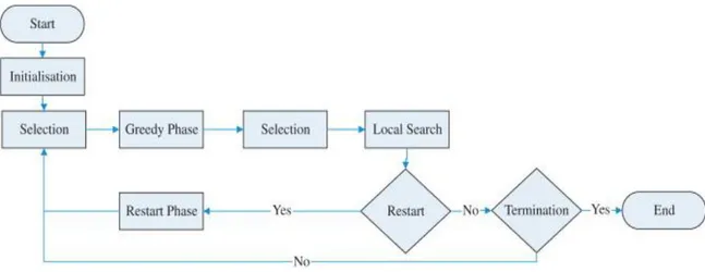
34 To give a general scheme about how the algorithm is divided, it can be broken into five phases:
1. Initialization. In this first phase, an initial set of good solutions is generated using two NEH heuristics, each one designed to attain good values for a specific criterion.
2. Selection. The second phase, chooses one solution from the current working set for the next phase.
3. Greedy phase. This phase represents the real core of the entire procedure. It is constituted by the two phases of destruction and
construction.
4. Local search. This phase is applied usually after greedy phase, over a selected element of the current working set.
5. Restart. This is the last phase procedure is implemented to prevent the algorithm from getting stuck in local optima.
35
Chapter 4
36
4.1 A model for the SDST Hybrid Flowshop
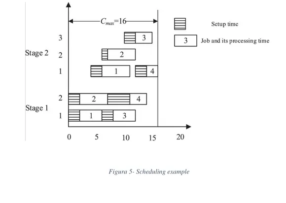
As an example, we consider a problem with four jobs (n = 4) and two stages (m = 2), with two machines at stage one (|M1| = 2) and three machines at stage two (|M2| = 3). The processing times and setup times are given in Tables 1 and 2, respectively. In this example we consider the special case of unrelated parallel machine where the processing time of the jobs on all parallel machines are identical. A schedule chart is shown in Figure 5.
J1 J2 J3 J4
Stage 1 4 5 4 3
Stage 2 5 5 3 2
Tabella 3 - Processing times example
Stage 1 Stage 2 Ji\Jj J1 J2 J3 J4 Ji\Jj J1 J2 J3 J4 J1 2 3 2 2 J1 2 3 2 2 J2 2 2 3 4 J2 2 1 3 4 J3 4 2 2 3 J3 3 3 2 3 J4 3 3 2 2 J4 4 3 2 2
37 Figura 5- Scheduling example
4.2 Encoding methods
Encoding method consists of representing a schedule by a string of decision variables, or saying, chromosome. A schedule is defined by indicating the start and finish times for each operation on the machine to which it is assigned. Since we are optimizing regular objectives like Setup Time and Total Tardiness, all operations are expected to be started as early as possible. There can be distinguished basically two types of encoding: a direct encoding, which usually involves large solution space, that may render inefficient the searching procedure. In fact, It has been demonstrated that the more detailed the encoding, the worse the results. Indeed, indirect encoding employing surrogate heuristics in the decoding procedures for completing the solution is usually much efficient than a direct encoding. For this reason, most of the researches use the following indirect encoding scheme: a solution is encoded as a job permutation.
38 Encoding representations can be farther classified into nine categories
Direct Encoding - Operation based - Job based
- Job pair relation based - Completion time based - Random keys
Indirect Encoding - Preference list based - Priority rule based - Disjunctive graph based. - Machine based.
Figura 6- Encoding/decoding classifications
These classification takes more sense when contextualized in GA environment with job shops and these nine categories can be grouped into the already mentioned two basic encoding approaches—direct and indirect. So the point is that In direct approach, a schedule is encoded as a chromosome and genetic operators are used to evolve better individual ones. Categories 1 to 5 are examples of this category. In case of indirect approach, a sequence of decision preferences will be encoded into a chromosome. In this, encoding, genetic operators are applied to improve the ordering of various preferences and a Πj schedule is then generated from the sequence of preferences. Categories 6 to 9 are examples of this category. Some words need to be spent on Random Keys Representation (RK), because more than others, it is used sometimes also in Hybrid Flow Shop environment. In this representation, each gene is represented with random numbers generated between 0 and 1. These random numbers in a given chromosome are sorted out and are replaced by integers and now the resulting order is the order of operations in a chromo- some. This string is then interpreted into a feasible schedule. Any violation of
39 precedence constraints can be corrected by a correction algorithm incorporated.
4.3 Decoding methods
Decoding is to derive a schedule from the encoded solution. The encoding procedures described does not contain all the required information and decision variables for constructing a HFS schedule. These missing
information like for example machine selection decisions, are determined by some heuristics during the decoding procedure. That’s why the solution quality strictly depends on the decoding method. Also in this case, the most used decoding methods are:
1) List scheduling (LS). It is a decoding method adopted in many researches (as shown in Table 1); an initial job list L1 is created in the first stage, according to some objective to optimize. Then jobs are picked out from L1 sequentially and scheduled as early as possible on the machine selected by a machine assignment rule. In the remaining stages, it is applied the same procedure as in stage 1 except that Li (i > 1) is created by the First-come-first-served (FCFS) rule, that is sorting the jobs increasingly by their completion time in the precedent stage. As a consequence, it happens than especially with increasing number of stages, the sequence of processed jobs can change stage by stage because each time, the next job of the list is scheduled on the machine that is available first. If a tie exists, then usually the job is scheduled on the machine with the smallest index. List schedules are also used in branch-and-bound algorithms for problems in which the set of list schedules is dominant, i.e., contains at least one optimal solution.
2) Permutation scheduling (PS). This method is similar to LS except that the job lists in each remaining stage are equal to π as well.
40 Both these methods are widely used in literature and in HFS environment. Anyway both these methods have drawbacks. When scheduling has to be done, the objective that is to be optimized is very crucial for deciding which process job has the priority to be processed first than others and these urgent jobs, called “hot jobs” must be completed as soon as possible. That’s why they are placed in the left part of the solution. Yet this is only for stage 1 but makes no guarantees for the subsequent stages where jobs are queued by the FCFS rule. For this reason, it is very difficult to control the propagation of the schedule, especially when a higher number of jobs in the sequence is considered. That’s why this kind of approach leads to the difficult handling of urgent jobs. If in the scheduling decision process, one wants to precisely define when a job will start and when it will finish, this become very hard to do when number of operations and number of jobs increases. Such we call the
controllability problem. On the contrary, this problem with PS this problem is
not present because we schedule the jobs in each stage by the same sequence
π. Yet, this leads to another problem: unnecessary machine idleness. More
specifically, when the sequence that jobs exiting from the stage is different from π, to schedule the jobs at the stage i by sequence π we have to delay the starting time of some jobs, which may lead to unnecessary machine idleness. So idleness will be higher when the processing times of the operations of each jobs are variable from one stage to another and also between the jobs themselves. It ends up with less tightness of the schedule, given this approach so static. We call this the tightness problem. In this research, literature review was conducted also to better understand which decoding method was the better to use in the application of this algorithm. As shown in the table, a resume of part of the investigated paper has been summarized.
41 T a b ell a 5 Res u me ta b le p er p a p er
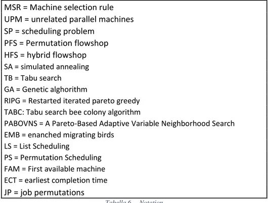
42 Here some notation used in table 5:
Tabella 6 -- Notation
This very small literature review, has been distinguished from the wider one conducted in chapter 2, because has the goal to identify some features especially concerning the encoding and decoding methods used.
As shown in the tables, different methods and approaches have been chosen, but encoding and decoding methods are essentially the same. In particular, job permutation represents the much used encoding method. As said before, this kind of indirect encoding is much more efficient. Indeed, no particular preference seems shown about the decoding method. Given that we are optimizing objectives like Total Tardiness and Total Setup Time, it is somehow logic to expect that, especially when the number of jobs is increasing, it can be much more important to have control on the jobs we are scheduling. Moreover, it is important to remember the assumption of unrelated parallel machines with machine eligibility. For completeness, also the machine selection criteria has been specified in the tables. It can be seen that the first
MSR = Machine selection rule UPM = unrelated parallel machines SP = scheduling problem PFS = Permutation flowshop HFS = hybrid flowshop SA = simulated annealing TB = Tabu search GA = Genetic alghorithm
RIPG = Restarted iterated pareto greedy TABC: Tabu search bee colony algorithm
PABOVNS = A Pareto-Based Adaptive Variable Neighborhood Search EMB = enanched migrating birds
LS = List Scheduling
PS = Permutation Scheduling FAM = First available machine ECT = earliest completion time
43 available machine rule is preferred, especially given that in most cases, the maximum makespan is the objective to minimize.
4.4 The restarted iterated pareto greedy
In the literature review, it has been already said like the Iterated Greedy procedure belogs to the class of the stochastic local search techniques (SLS). Now, similarly to [7], we propose a procedure named Restarted Iterated
Pareto Greedy (RIPG). The logic behind this algorithm is very simple: a greedy
multi-objective strategy is iteratively applied over a set of non-dominated solutions. The proposed RIPG is an extension of the above described IG. In fact, the main drawback of IG procedure is that they are prone to get stuck in local optimum solutions. The reason lies behind their very nature as they are greedy methods. RIPG is no different. To avoid this potential problem, we have included a simple, yet reliable restart phase. This procedure merely consists of storing all the elements of the current working set in a separate archive and then creating a new random working set of 100 elements. The main advantage of this restart procedure is that it is a very fast way to introduce diversification inside our metaheuristic scheme, whereas its main inconvenience consists of the difficulty in choosing of a suitable restarting criterion. To give a general scheme about how the algorithm is divided, it can be broken into five phases:
1) Initialization. In this first phase, an initial set of good solutions is generated using two NEH heuristics [127], each one designed to attain good values for a specific criterion. The first one for the Total Tardiness objective (TT) and the second one for the minimization of the Total Setup Time (TST). After that, the remaining four phases are iteratively repeated and constitute the main loop of the algorithm.
44 2) Selection. The second phase, chooses one solution from the current working
set for the next phase. The procedure adopted to do this is the so called Modified Crowding Distance Assigned procedure (MCDA). This method was originally presented in [86] has been developed in order to carry out the selection process. At each solution is assigned a value (Crowding Distance) which depends on the normalized Euclidean distances between it and the solutions that precedent. The main difference between the classical one and this new modified version resides in the fact that the modified procedure considers the number of times each solution has been already selected in previous iterations (Selection Counter), and uses this information to calculate the Modified Crowding Distance (MCD). This modification prevents allocating computing resources to search the same regions. The element with the highest value of MCD is selected as the starting point for the Greedy or local search phases.
3) Greedy phase. This phase represents the real core of the entire procedure. It is constituted by the two phases of destruction and construction. The destruction procedure is applied to a permutation π of n jobs and it chooses randomly, without repetition d jobs. These d jobs are then removed from π in the order in which they were chosen. The result of this procedure are two subsequences, the first being the partial sequence πD with n − d jobs, that is the sequence after the removal of d jobs, and the second being a sequence of
d jobs, which we denote as πR. πR contains the jobs that have to be reinserted into πD to yield a complete candidate solution in the order in which they were removed from π. The construction phase starts with subsequence πD and performs d steps in which the jobs in πR are reinserted into πD.. This process is iterated until πR is empty.
45 4) Local search. This phase is applied usually after greedy phase, over a selected
element of the current working set.
5) Restart. This is the last phase procedure is implemented to prevent the algorithm from getting stuck in local optima.
In Figure 1 it is presented a general scheme of the procedure. The detailed procedure will be described later in chapter 4.
Figura 7 - RIPG scheme
4.4.1 The inizitalization phase
Conducetd experiments done in literature, clearly showed that a good initial working set greatly improves the quality of RIPG. This is certainly expected as it is also the case with the single-objective PFSP. In the first phase, an initial set of good solutions is generated using two well-known NEH heuristics, each one designed to attain good values for a specific criterion. In fact, it is intuitive that the generated initial solutions represent the starting point on which more complex elaborations had be done. From this perspective, the initial solutions play an underlying role in creating a high performing algorithm. By the way,
46 since our analysis focuses on reaching not one but two objectives, the choice in the adopted heuristics was due to choose heuristics the return of good enough solutions but that also ensure a sufficient level of diversity. Further considerations are needed. First, it is not sure that these initial solutions will be well spread in the Pareto front. Also, this algorithm methodology adopts the selection process and the greedy phase many times. This approach is capable of greatly improving solutions. Selecting only one of the initial solutions for the greedy phase could have a negative result: all other initial solutions could be dominated after this phase. As a result, there is loss of diversity and coverage in the Pareto front. So, discarding some initial solutions can be a mistake because you lose the possibility to go toward promising directions. That’s why, in the first step of the RIPG, all initial solutions are processed by the greedy phase, without applying the selection operator, and for each one, a non-dominated set is obtained.
So summarizing, the results of this heuristics generates the Initial Solution Set (ISS), making use of two well-known NEH heuristics, will soon generate respectively two initial solutions, one optimizing the objective of the Total Tardiness (TT) and one optimizing the objective of Total Setup Time (TST). This is the starting point of the procedure, which will step by step be replaced by better solutions. In a first step, all initial solutions are processed by the Greedy
Phase one by one. The obtained solutions of this process are added to the ISS
and then, the dominated ones are removed and the initial current working set
(CWS) is conformed. The word “dominated” refers to the concept of Pareto
dominance. The concept of Pareto dominance is of extreme importance in
multi-objective optimization, especially where some or all of the objectives and constraints are mutually conflicting. In such a case, there is no single point that yields the "best" value for all objectives and constraints. Instead, the best solutions, often called a Pareto or non-dominated set, are a group of solutions such that selecting any one of them in place of another will always sacrifice quality for at least one objective or constraint, while improving at least one other. In our case, the aim behind this policy, adopted in the initial phase, is
47 to avoid that a likely large improvement during the initial iterations might generate a set of solutions that dominate the remaining initial solutions, impoverishing the quality and diversity of the working set too early. At each iteration of the algorithm, the selection phase is applied. Its role is to point the search towards promising directions. Selection achieves this goal by choosing one solution from the current working set on the basis of considerations related to their quality. The detailed description of it, will be done later in the text. In this way, only those solutions that are more likely to increase the quality of the current working set will be kept, speeding up the whole search process. After this initialization, the working set of non-dominated solutions is ready for the main algorithm phases. The diagram and the pseudocode is in [APPENDIX - 8.1].
1
• NEH_EDD to generate two initial solutions, one for
each objective to optimize, constiututing CWS
2
• Greedy phase of the CWS
3
• Filtering and keep the non dominated solutions in
the CWS.
48
4.4.2 The selection phase
As already mentioned before, a selection phase is often applied before the greedy phase to choose which solutions are more convenient to elaborate, based on a criteria presented by [124], for the first time. The aim of the selection phases to select a candidate solution belonging to a less crowded region of the Pareto front and at the same time has already been selected a small number of times To do so, a modified version of the Crowding Distance
Assignment (CDA) procedure, has been developed in order to carry out the
selection process. The original CDA method divides the working set into dominance levels, i.e., the set of non-dominated solutions form the first-level Pareto front. Once we remove these elements, we have another non-dominated set of solutions, which correspond with the second-level Pareto front. This procedure is repeated until all solutions are assigned to a Pareto front. Here, we do not consider this distinction in levels, because it’s not useful for our objectives. Afterwards, it assigns to each solution a value (Crowding Distance) dependent on the normalized Euclidean distances between it and the solutions that precede and follow it. Such technique favors the selection of the most isolated solutions of the first frontier This CDA will represent a sort of priority value and create a hierarchy inside the field of the solutions. Therefore, applying the standard Crowding Distance procedure results in an algorithm that gets easily stuck, as if no improvements are found after the greedy and local search phases, the Pareto fronts do not change and the same solution is selected repeatedly. To avoid this, we add a selection counter (n_sel) to each solution which counts the number of times each solution has been selected. This represents the main difference between the normal CDA procedure and the MCDA adopted here. Then, it uses this information to calculate the Modified Crowding Distance (MCD). At the end, the solution with the highest value of MCD is selected as the starting point for the Greedy or the local search phases. The use of such an operator demonstrated, in preliminary experiments, to significantly improve the Pareto front in terms of
49 quality and spread of its solutions. The diagram of this phase and the pseudocode are presented in [APPENDIX – 8.2] .
4.4.3 The greedy phase
This is the heart and most innovative part of the algorithm even though the structure of the original IG is still kept unchanged. However, there are some important differences between the greedy phase adopted in the first original IG procedure, and the one adopted here inside the RIPG. In particular, in the original procedure where only one partial solution is maintained and a NEH-like greedy heuristic is applied in one unique step at each iteration of the algorithm. The innovation here, is that, in RIPG, the Greedy phase becomes an iterative process, that works with a set of partial solutions and returns a set of non-dominated permutations. Let’s go into the details; the Greedy phase can be basically divided into two steps: In the first one, called Destruction Phase, a block of d consecutive elements is randomly removed from the MCDA-selected solution. This is the other important difference with the original GP because there the removal was not carried out by groups of elements. So, The Destruction step chooses a randomly a starting position k, and a block of d consecutive elements are removed from the selected solution. This 𝑘 parameter is of great importance and will be one of the parameters that will be tuned afterwards in the calibration of the algorithm. The second step, called Construction phase, iteratively reconstructs the solution by reinserting, one by one, all the d removed elements into all possible positions of a group of partial solutions. This inserting scheme was already effectively used in [125] and it is possible thanks to the use of Pareto dominance. At each step, a new set of partial solutions is generated. More specifically, let n be the length of the initial solution and d the size of the block of removed elements. During the first iteration, the first of the d removed elements is inserted in all possible positions of the partial solution. This generates (𝑛 − 𝑑 + 1) new partial solutions. The next removed element, will