Universit`
a degli Studi di Pisa
FACOLT `A DI SCIENZE MATEMATICHE, FISICHE E NATURALI
Corso di Laurea in Matematica
Delay-Induced Oscillatory Dynamics
of Tumor-Immune System Interaction.
31 Ottobre 2008
Candidata: Francesca Gatti Relatori:
Dott. Alberto d’Onofrio Prof.ssa Paola Cerrai
Controrelatore: Prof. Vieri Benci
Contents
Introduction 4
1 Basic theory of delay differential equations 7
1.1 Basic properties . . . 7
1.2 Dynamical systems and invariance . . . 11
1.3 Stability theory . . . 14
1.3.1 Stability and maximal invariant sets . . . 14
1.3.2 The method of Liapunov functionals . . . 16
1.3.3 Razumikhin theorems . . . 19
1.4 Periodic solutions of autonomous equations - Hopf bifurcations. 20 1.5 Characteristic equation analysis . . . 22
1.5.1 Discrete delay- second order equations . . . 24
1.5.2 Distributed delay - Linear chain trick . . . 27
1.6 Delayed logistic equation . . . 28
2 Tumor-Immune System Interaction and Mathematical Mod-els 31 2.1 Tumor, Immune system, and their interaction . . . 31
2.2 Immunotherapy . . . 34
2.3 Mathematical Models in Cancer Research . . . 34
2.3.1 Some relevant models . . . 35
3 A New Nonlinear Model of Tumor-Immune System Inter-action 43 3.1 Nullclines . . . 44
3.1.1 Disease Free Equilibrium . . . 45
3.1.2 Equilibria with non null disease . . . 46
3.2 Limit cycles . . . 47
3.3 Unique non-DFE equilibrium . . . 48
3.4 Examples . . . 48
3.5 Therapy . . . 49
3.5.1 Constant therapy . . . 50
3.5.2 Periodic therapy . . . 51 3
CONTENTS CONTENTS
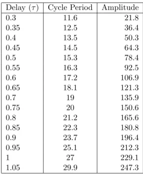
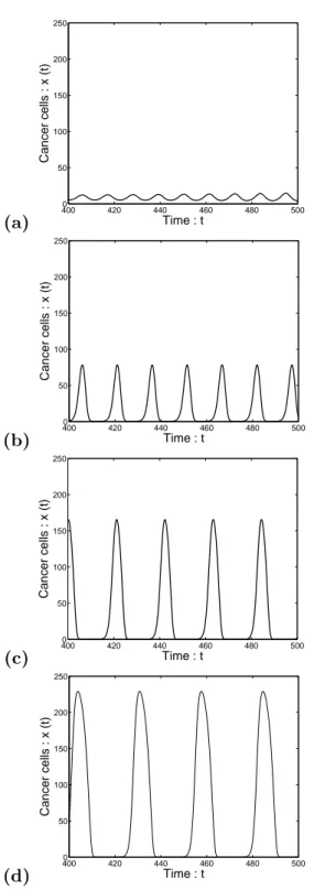
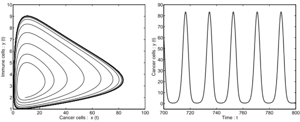
3.5.3 Numerical results . . . 53
4 Mathematical analysis of the effect of delays between tumor growth and stimulation of immune cells proliferation 59 4.1 Fixed lag delay . . . 60
4.1.1 EQ is LAS and q0(x e) ≤ 0 . . . 62
4.1.2 EQ is LAS and q0(x e) > 0 but S < 0 . . . 63
4.1.3 EQ is LAS but N S < 0 . . . 63
4.1.4 EQ is unstable and there are no limit cycles . . . 65
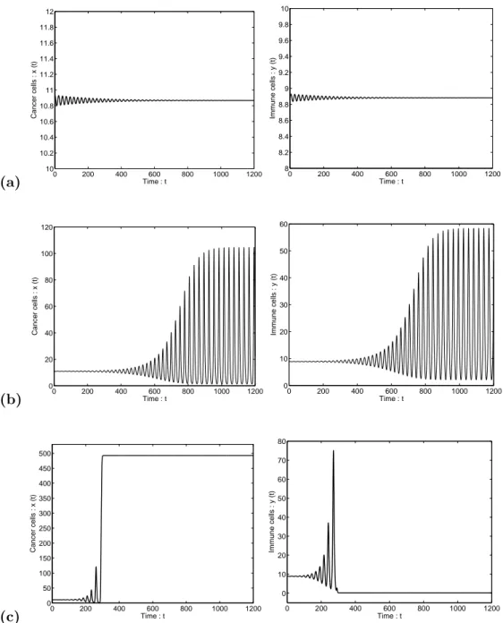
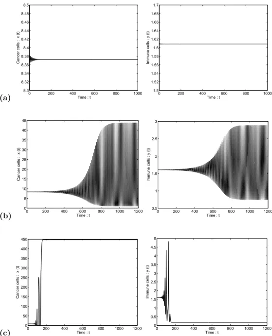
4.1.5 EQ is unstable, H + R > 0 but HR − N S − N Q > 0 . 65 4.2 Numerical simulations . . . 66 4.2.1 EQ is LAS and q0(x e) ≤ 0 . . . 67 4.2.2 EQ is LAS and q0(x e) > 0 but S < 0 . . . 72 4.2.3 EQ is LAS but N S < 0 . . . 74
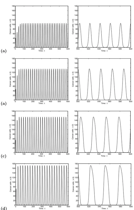
4.2.4 EQ is unstable and there are limit cycles: H + R > 0 but HR − N S − N Q > 0 . . . 76
5 Distributed delay 79 5.1 Exponentially distributed delay . . . 80
5.1.1 Numerical results . . . 85
5.2 Strong Erlangian delay . . . 90
5.2.1 Numerical results . . . 91
6 Interactions between delay and therapy 95 6.1 Discrete delay; no limit cycle model . . . 96
6.2 Discrete delay; limit cycle model . . . 100
6.3 Exponentially distributed delay . . . 103
Bibliografia 109
Introduction
In the latest years, among scientific literature, many papers have been pub-lished presenting mathematical models in cancer research field. They exam-ine different biological aspects and use different mathematical tools.
In this work we focus on deterministic models concerning tumor-immune system interaction, based on ordinary differential equations or delay differ-ential equations. It has been done a critical reading of the existing literature drawing our attention on a special family of models that we have then gen-eralized. From this departing point we studied how adding of a delay term can affect the system dynamics.
In biological phenomena, especially in tumor growth and development, and in the tumor-immune system interaction, delays can be due to many reasons (times of cellular division and displacement in the organism, time lags from signals sending to their reception, times of synthesis and transport of proteins, ... ), but often they are neglected in mathematical models that are formulated using ordinary differential equations.
In this work, applying the theory of delay differential equations, we have analyzed models behavior both with discrete and distributed delay, aiming to stress the possibility of these systems to show an oscillatory dynamics. As far as the examined literature is concerned, oscillations experimentally observed in tumor growth are a feature hard to explain for scientists.
This research is mainly done looking for Hopf bifurcations. We use delay as bifurcating parameter, in order to study if and how the delay can influence the stability of the system and its dynamics. We proved that including a delay term may cause - under some conditions - changes in the stability of equilibrium points. Moreover, for some delay values, models can exhibit limit-cycles that are not present in systems without delay.
The study has been run both analytically and numerically: we have been dealing with different realistic examples whose parameter values, taken from literature, were fitted from data sampled in clinical experiments. The obtained results have been discussed both from a mathematical point of view and for their medical-biological meaning. Finally, some simulations have been conducted on a system to which has been added a term representing delivery of a therapy (immunotherapy).
dif-CONTENTS CONTENTS
ferent mathematical expressions, primarily focusing our numerical analysis on the more relevant case of boli-based therapy.
As a result, varying therapy parameters, such as administration and clearance time, we observed very interesting behaviors in model dynamics, changes in stability properties and also resonance effects.
Contents are organized into six chapters.
The first reports basic results of theory of delay differential equations and methods of analysis that are then utilized in following chapters.
In the second chapter topics of tumor-immune system interaction and mathematical modeling are introduced and some relevant models are suma-rized and discussed.
In third chapter a new model of tumor-immune system interaction is presented and studied both analytically and numerically showing some bi-logically meaningful examples.
Then the issue of immunotherapy is taken into account adding to the system a treatment term and studying its behavior.
The fourth and fifth chapter are the core of this work. In these chapters a delay term is added to model introduced in third chapter and obtained delayed systems are studied analytically, with the aim to point out changes in stability of equilibrium points, Hopf bifurcations and periodic dynamics. Then delayed systems are studied numerically taking parameters within a range of biological significance. In fourth chapter the delay term introduced is a fixed lag delay, whereas in fifth chapter distributed delays are considered. Finally the sixth chapter deals with immunotherapy in delayed models. A numerical analysis was carried out for systems with delay and treatment terms and many examples are showed and discussed, pointing out interesting biological and mathematical features.
Chapter 1
Basic theory of delay
differential equations
In many real processes, especially in the medical/biologic field, the dynam-ics depends not only on the present state of the system, but also on the past history of state variables. Modeling situations in which past history is not negligible necessarily leads to the study of delay differential equations (DDE).
In this chapter we report a survey of the theory of DDE. In the first part we give some basic definitions, existence, uniqueness and stability results. Then we treat existence and stablity of periodic solutions stating the Hopf Theorem for DDE.
Finally we describe some methods to study stability of delay system. In the last chapter of this work we will deal with that again to analyze stability properties and the occurrence of Hopf bifurcations in a family of models of tumor-immune system interaction.
The following text [1] may be consulted on this topic; it exposes an exhaustive theory of delay differential equations. In [2], [3] the matter is handled paying special attention to the biological applications. Interesting sections on equation with delay can also be found in [4] and [7].
1.1
Basic properties
Let r ≥ 0 be a real number and C = C([−r, 0], Rn) the Banach space of continuous functions mapping [−r, 0], into Rnand the supremum norm. For
σ ∈ R, A ≥ 0, x ∈ C([σ − r, σ + A], Rn), and t ∈ [σ, σ + A], we define x
t∈ C as xt(θ) = x(t + θ), θ ∈ [−r, 0].
Let Ω be a subset of R × C, f : Ω → Rn a given function and denote the right-hand derivative by a dot: ˙.
1.1
CHAPTER 1. BASIC THEORY OF DELAY DIFFERENTIAL EQUATIONS
the form:
˙x(t) = f (t, xt). (1.1) A function x is said to be a solution of (1.1) on [σ −r, σ +A) if there is σ ∈ R,
x ∈ C([σ − r, σ + A), Rn), (t, x
t) ∈ Ω and xt satisfies (1.1) for t ∈ [σ, σ + A). Given σ ∈ R, ϕ ∈ C we say that x(σ, ϕ) is a solution of (1.1) with initial value ϕ in σ, or a solution through (σ, ϕ), if there is A > 0 such that x(σ, ϕ) is a solution of (1.1) on [σ, σ + A) and xσ(σ, ϕ) = ϕ. According to (1.1) the right-hand derivative of the solution x at t is determined by t and by the restriction of x(t) to the interval [t − r, t]. If the solution is unique, then for every t ≥ 0 we can define:
T (t) : ϕ → xt(σ, ϕ), (1.2)
that maps C into itself. T (t) is called the solution map of ½
˙x(t) = f (t, xt), t ≥ σ,
xσ = ϕ. (1.3)
We say that the equation (1.1) is linear if f (t, xt) = L(t, xt) + h(t), where
L(t, xt) is linear in xt; linear homogeneous if h(t) ≡ 0 and linar
nonho-mogeneous if h(t) 6= 0. We say that (1.1) is autonomous if f (t, xt) = g(xt)
where g does not depend on t, otherwise we say that (1.1) is nonautonomous. The DDE (1.1) includes many classes of equations such as ODE if r = 0, in fact, in this case xtis defined on the interval consisting of the single point 0 and xt= xt(0) = x(t). It includes also differential-difference equations of the form:
˙x(t) = f (t, x(t), x(t − r1), ..., x(t − rm)) (1.4) where 0 ≤ ri ≤ r for i = 0, ..., m. Here f is a function of nm + 1 real variables and we say that there are m delays in the equation, each less than
r. The delays rimay also depend on the time t. Finally, DDE (1.1) includes
integro-differential equations: ˙x(t) =
Z 0 −r
g(t, x(t), θ, xt(θ))dθ (1.5)
where g is a function of 2n + 2 variables.
We observe that, if we assume f continuous, finding a solution of (1.1) through (σ, ϕ) ∈ R × C is equivalent to solving the integral equation:
½
x(t) = ϕ(0) +Rσtf (s, xs)ds t ≥ 0
xσ = ϕ (1.6)
Theorems of existence and uniqueness of solutions hold and are more or less analogous to the corresponding results for ODE.
CHAPTER 1. BASIC THEORY OF DELAY DIFFERENTIAL
EQUATIONS 1.1
Theorem 1.1.1. Suppose Ω is an open subset in R × C and f is continuous
in Ω. If (σ, ϕ) ∈ Ω, then there is a solution of (1.1) through (σ, ϕ).
Definition 1.1.1. We say that f (t, ϕ) is Lipschitz in ϕ in a compact subset
K in R × C if there is a constant k > 0 such that ∀ (t, ϕi) ∈ K (i = 1, 2)
|f (t, ϕ1) − f (t, ϕ2)| ≤ k|ϕ1− ϕ2|
Theorem 1.1.2. Suppose Ω is an open subset in R × C, f : Ω → Rn is
continuous and f (t, ϕ) is Lipschitz in ϕ in every compact of Ω. If (σ, ϕ) ∈ Ω, then there is a unique solution of (1.1) through (σ, ϕ).
Also theorems about continuous dependence on initial values and on the continuation of solutions hold and are analogous to the corresponding results for ODE, but in some cases one has to assume that f is completely continuous.
Theorem 1.1.3. Suppose Ω ⊆ R × C is open, (σ, ϕ) ∈ Ω, f ∈ C(Ω, Rn),
and x is a solution of (1.1) through (σ, ϕ) which exists and is unique on
[σ − r, b], b > σ − r. Let W ⊆ Ω be the compact set defined by
W = {(t, xt) : t ∈ [σ, b]}, and let V be a neighborhood of W on which f is
bounded. If (σk, ϕk, fk), k=1,2,..., satisfies σk → σ, ϕk → ϕ, and |fk −
f |V → 0 as k → ∞, then there is a K such that for k ≥ K each solution
xk = xk(σk, ϕk, fk) through (σk, ϕk) of ˙x(t) = fk(t, x
t) exists on [σk− r, b]
and xk → x uniformly on [σk− r, b]. (Since all xk may not be defined on
[σk− r, b], by xk → x uniformly on [σk− r, b] we mean that for any ε > 0
there is a k1(ε) such that xk(t), k ≥ k
1(ε) is defined on [σk− r + ε, b] and
xk→ x uniformly on [σk− r + ε, b].)
Let x be a solution of (1.1) on the interval [σ, a), a > σ. We say that ˆx
is a continuation of x if there is a b > a such that ˆx is defined on [σ − r, b),
coincides with x on [σ − r, a), and x satisfies the equation (1.1) on [σ, b). A solution x is said noncontinuable if no such continuation exists, that is the interval [σ, a) is the maximal interval of existence of the solution x. The existence of a noncontinuable solution is a consequence of Zorn’s lemma. Theorem 1.1.4. Suppose Ω open in R × C, f : Ω → Rn completely
con-tinuous and let x be a noncontinuable solution of (1.1) on [σ − r, b). Then
for any closed and bounded set U ∈ R × C, U ⊂ Ω, there is a tU such that
(t, xt) 6∈ U for tU ≤ t < b.
The previous theorem says that solutions of equation (1.1) exist for any time t ≥ σ or become unbounded (with respect to Ω) in finite time and it gives conditions under which the trajectory (t, x) in R × C of a noncon-tinuable solution of [σ, b) approaches the boundary of Ω as t → b−. If the condition that f is completely continuous is not imposed, then it is conceiv-able that the trajectory {(t, xt) : σ ≤ t < b} itself is a closed bounded subset
1.1
CHAPTER 1. BASIC THEORY OF DELAY DIFFERENTIAL EQUATIONS
of Ω; that is the curve (t, x(t)) oscillates so badly as a subset of R × Rn that there are no limit points of (t, xt) in R × C as t → b−.
Theorem 1.1.5. Suppose that x : [−r, α) → Rn, r > 0, α finite, is an
arbitrary bounded continously diffrentiable function satisfying the property
that x(t) does not approach a limit set as t → α−. Then there is a continuous
function f : C → Rnsuch that x is a noncontinuable solution of the DDE(f )
on [−r, α).
The theorem on continuation of solutions states that a noncontinuable solution of a DDE(f ) must leave every bounded and closed set W in the domain Ω of the equation, supposing that f is completely continuous on Ω. A continuous function on Ω is not necessarily completely continuous on Ω if r > 0, that is if C is infinite-dimensional.
The theorem on continuation of solutions does not hold if f is not completely continuous.
For the ode ½
˙x(t) = f (t, xt)
x(0) = x0 (1.7)
if f ∈ Ck, k ≥ 0 then the solution x(t) of (1.7) is itself in the space Ckin its maximal interval of existence. For the equation (1.1) the same is true only for some values of t. In the Theorem 1.1.3 were given sufficient conditions to assure that the solution x(σ, ϕ, f ) of a DDE(f ) depends continuously on (σ, ϕ, f ). Here we state some results on the differentiability of solutions with respect to (σ, ϕ, f ).
Theorem 1.1.6 (Smoothing property). Let x(t) be the solution of ½
˙x(t) = f (t, xt)
xσ = ϕ, ϕ ∈ C, (1.8)
where f ∈ Ck, k ≥ 1 and let I = [σ, t
x) be the maximal interval of existence
for x(t). Then x(t) ∈ Cl on [σ + lr, t
x) for l=0,1,...k.
In other words x(t) is even more regular increasing T . If f ∈ C1, Φ ⊂ C
is a bounded closed set and T (t)Φ ≡ Sϕ∈ΦXt(σ, ϕ) is a bounded set for
t ≥ σ + r, then T (t)Φ is compact as t ≥ σ + r.
If Ω is open in R × C, let Cp(Ω, Rn), p ≥ 0 be the space of functions mapping Ω in Rnand bounded continuously differentiable up to order p with respect to ϕ on Ω. The space Cp(Ω, Rn) becomes a Banach space with the norm of supremum over all derivatives up to order p.
Next theorem follows from contraction principle in Banach spaces. Theorem 1.1.7. If f ∈ Cp(Ω, Rn), p ≥ 1, then the solution x(σ, ϕ, f )(t) of
CHAPTER 1. BASIC THEORY OF DELAY DIFFERENTIAL
EQUATIONS 1.2
to (ϕ, f ) for t in a compact set in the domain of x(σ, ϕ, f ). Moreover, for any
t ≥ σ the derivative of x with respect to ϕ: Dϕx(σ, ϕ, f )(t) is a linear
oper-ator from C to Rn, Dϕx(σ, ϕ, f )(σ) = I, the identity, and Dϕx(σ, ϕ, f )ψ(t)
for any ψ ∈ C satisfies the linear variational equation:
y(t) = Dϕf (t, xt(σ, ϕ, f ))yt.
Moreover, for any t ≥ σ, Dfx(σ, ϕ, f )(t) is a linear operator from Cp(Ω, Rn)
in Rn, Dfx(σ, ϕ, f )(σ) = 0 and Dfx(σ, ϕ, f )g(t) for g ∈ Cp(Ω, Rn) satisfies
the linear variational equation:
˙z(t) = Dϕf (t, xt(σ, ϕ, f ))zt+ g(t, xt(σ, ϕ, f )).
1.2
Dynamical systems and invariance
For autonomous ODEs, bounded solutions have nonempty, compact, con-nected an invariant Ω-limit sets. Similar results hold also for DDEs. Definition 1.2.1 (Process). Let X be a Banach space, u : R × X × R+→ X
a given mapping and let us define U (σ, t) : X → X for σ ∈ R, t ∈ R+ by
U (σ, t)x = u(σ, x, t). A process on X is a mapping u : R × X × R+ → X
satisfying the following properties:
(i) u is continuous; (ii) U(σ,0)= I;
(iii) U(σ+s,t)U(σ,s)= U(σ, s+t).
A process u is said p-periodic, p > 0 if U(σ+p,t)=U(σ,t) for σ ∈ R, t ∈ R+.
Suppose f : R × C → Rnis completely continuous and let x(σ, ϕ) be the solution of DDE(f):
˙x(t) = f (t, xt), xσ = ϕ. (1.9) We assume that x is uniquely defined for t ≥ σ. Theorem 1.1.3 implies that
x(σ, ϕ)(t) is continuous in σ, ϕ, t for σ ∈ R, ϕ ∈ C e t ≥ σ. Define
u(σ, ϕ, τ ) = xσ+τ(σ, ϕ), (σ, ϕ, τ ) ∈ R × C × R+,
then u is a process on C. Moreover, let T (t, σ) be the solution operator for (1.9) defined by:
T (t, σ)ϕ = xt(σ, ϕ);
then U (σ, τ ) = T (σ + τ, σ), where U (σ, τ )ϕ = u(σ, ϕ, t).
We will say that u(σ, ϕ, τ ) is the process generated by the DDE(f ).
If f (σ + p, ϕ) = f (σ, ϕ) p > 0 ∀(σ, ϕ) ∈ R × C then the process generated by the DDE(f ) is p-periodic.
1.2
CHAPTER 1. BASIC THEORY OF DELAY DIFFERENTIAL EQUATIONS
Definition 1.2.2. A process is said a (continuous) dynamical system, or
an autonomous process, if U (σ, t) is indipendent by σ; that is if
T (t) = U (0, t), t ≥ 0,
then T(t)x is continuous for (t, x) ∈ R+× X,
T (0) = I, T (t + τ ) = T (t)T (τ ), t, τ ∈ R+.
We also call T (t), t ≥ 0 a (continuous) dynamical system.
If S : X → X is a continuous map, the family ©Sk, k ≥ 0ª of iterates
of S is said a discrete dynamical system. If u is a p-periodic process and
S = U (0, p), then Sk= U (0, kp). We refer to this discrete dynamical system
as the discrete dynamical system generated by the map of the p-periodic process.
In a process u(σ, x, t) can be considered as the state of the system at time σ + t when initial state at time σ is x.
Definition 1.2.3. Suppose that u is a process in X. The trajectory τ+(σ, x)
through (σ, x) ∈ R × X is:
τ+(σ, x) =©(σ + t, U (σ, t)x) : t ∈ R+ª⊂ R × X.
The orbit γ+(σ, x) through (σ, x) is:
γ+(σ, x) =©U (σ, t)x : t ∈ R+ª⊂ X. If H is a subset of X, then τ+(σ, H) = [ x∈H τ+(σ, x), γ+(σ, H) = [ x∈H γ+(σ, x).
A point C ∈ X is said an equilibrium (or critical) point of a process u if
U (σ, t)C = C for t ∈ R+. If there is σ ∈ R, p > 0, x ∈ X such that
U (σ, t + p)x = U (σ, t)x for any t ∈ R+ then τ+(σ, x) is said p-periodic.
If u is a process p-periodic on X, then the trajectory τ+(σ + kp, x) for
any integer k ∈ R is the traslated along reals of kp of the trajectory τ+(σ, x).
The orbits satisfy γ+(σ + kp, x) = γ+(σ, x) for any integer k ∈ R . If u is a
dynamical system on X then τ+(σ + s, x) is the traslated by s of τ+(σ, x)
for any s ∈ R and γ+(σ, x) = γ+(0, x) for any s ∈ R. In this last case we
simply write γ+(x) for orbits.
Lemma 1.2.1. For a continuous dynamical system, a trajectory is p-periodic
if and only if the corresponding orbit is a closed curve. For a p-periodic pro-cess u, a trajectory through (σ, x) is kp-periodic for a positive integer k if
CHAPTER 1. BASIC THEORY OF DELAY DIFFERENTIAL
EQUATIONS 1.2
Lemma 1.2.2. Let {T (t) : t ≥ 0} be a dynamical system on X. If there are
sequences {xn} ⊆ X, {ωn} ⊆ (0, ∞) satisfying T (ωn)xn = xn, ωn → 0
when n → ∞ and some subsequence of {xn} converges to x0, then x0 is an
equilibrium point.
Definition 1.2.4. Suppose that u is a process on X. A point y ∈ X is said
to be in the ω-limit set ω(σ, x) of an orbit γ+(σ, x) if there is a sequence
tn→ ∞ as n → ∞ such that U (σ, tn)x → y as n → ∞. A point y ∈ X is
said to be in the α-limit set α(σ, x) of an orbit γ−(σ, x) =St≤0U (σ, t)x if
U (σ, t) is uniquely defined for t ≤ 0 and there is a sequence tn → −∞ as
n → ∞ such that U (σ, tn)x → y as n → ∞. Equivalently we have: ω(σ, x) = \ t≥0 [ τ ≥t U (σ, τ )x, (1.10) α(σ, x) = \ t≤0 [ τ ≤t U (σ, τ )x, (1.11)
For any subset H ⊆ X we define ω- and α-limit sets of H, ω(σ, H), α(σ, H) by replacing x by H in (1.10), (1.11) respectively. If©Tk, k ≥ 0ªis a discrete dynamical system of X, and H ⊆ X, then the ω-limit set of H is defined as:
ω(H) = \
j≥0 [ n≥j
TnH,
and the α-limit set of H is defined as:
α(H) = \
j≤0 [ n≤j
TnH,
provided that TnH is well defined for any n ≤ 0. For autonomous DDE(f ),
½
˙x(t) = f (xt),
xσ = ϕ,
we have that ω(σ, x) = ω(x) is independent on σ. So y ∈ ω(x) (resp. α(x)) if and only if there is a sequence tn→ ∞ (resp. −∞) as n → ∞ such that
lim
n→∞xtn(σ, ϕ) = y. (1.12) Definition 1.2.5. If u is a process on X, then an integral of the process on R
is a continuous function y : R → X such that for any σ ∈ R, τ+(σ, y(σ)) =
{(σ + t, y(σ + t)) : t ≥ 0}. An integral y is an integral through (σ, x) ∈ R×X if y(σ) = x. An integral set on R is a set M in R × X such that for any
(σ, x) ∈ M there is an integral y on R through (σ, x) and (s, y(s)) ∈ M for
1.3
CHAPTER 1. BASIC THEORY OF DELAY DIFFERENTIAL EQUATIONS
Definition 1.2.6. If {T (t), t ≤ 0} is a dynamical system on X, then a set
Q ⊆ X is said invariant if T (t)Q = Q for t ≥ 0. This is equivalent to saying that through every point x ∈ Q there is an integral y through (0, x) such that y(s) ∈ Q, s ∈ R.
Definition 1.2.7. If u is a dynamical system on X, then a subset Q ⊆ X
is said to be a positively (negatively) invariant set for u if for any point
x ∈ Q, γ+(0, x) ⊂ Q (if U (σ, t) is well defined for t ≤ 0 and γ−(0, x) =
{U (σ, t)x : t ≤ 0} ⊂ Q).
Q is said an invariant set of u if T (t)Q ≡Sx∈QT (t)x = Q for every t ≥ 0.
Theorem 1.2.3. If an autonomous DDE(f) generates a dynamical system
and γ+(ϕ) is a bounded orbit, then ω(ϕ) is nonempty, compact, connected
and invariant. If H ⊆ C is connected and γ+(H) is bounded the same
conclusion is true for ω(H).
1.3
Stability theory
1.3.1 Stability and maximal invariant sets
Definition 1.3.1. For a given process u on X and a given σ ∈ R, we say
a set M ⊂ R × X attracts a set H ⊂ X in σ if, for any ε > 0, there is a t0(ε, H, σ) such that (σ + t, U (σ, t)H) ⊂ B(M, ε) for t ≥ t0(ε, H, σ). If M
attracts a set H in σ for every σ ∈ R, we say M attracts H.
Definition 1.3.2. For a given process u on X and a given σ ∈ R, we say
a set M ⊂ R × X is stable in σ if, for any ε > 0, there is a δ(ε, σ) > 0 such that (σ, x) ∈ B(M, δ(ε, σ)) implies that (σ + t, U (σ, t)x) ∈ B(M, ε) for t ≥ 0. The set M is said stable if it is stable in σ for any σ ∈ R. The set M is said unstable if it is not stable. The set M is said uniformly stable if it is stable and the number δ in the definition is independent on σ. The set
M is said asymptotically stable in σ if it is stable in σ and there is a ε0(σ)
such that (σ + t, U (σ, t)) → M as t → ∞ for (σ, x) ∈ B(M, ε0(σ)). The set
M is said uniformly asymptotically stable if it is uniformly stable and there
is a ε0 > 0 such that for every η > 0, there is t0(η, ε0) with the property
that (σ + t, U (σ, t)) ∈ B(M, η) for t ≥ t0(η, ε0) and for every x such that
(σ, x) ∈ B(M, ε0).
If a process is generated by an ODE in Rn, then M ⊂ R × Rn stable in a given σ ∈ R implies that M is stable in every σ ∈ R, that is M is stable. This result does not hold for more general processes, in particular it is not true for DDE.
It is difficult to determine when stability in σ is equivalent to stability. From a practical point of view, it is not so relevant to consider systems that are stables in σ but there are not stables. Therefore this weaker concept will not be discussed in detail.
CHAPTER 1. BASIC THEORY OF DELAY DIFFERENTIAL
EQUATIONS 1.3
Suppose now that u is a p-periodic process, K ⊂ X is a compact set, and that M ⊂ R × K attracts compact sets of X. For any σ ∈ R, let us consider the discrete dynamical system©Uk(σ, p), k ≥ 0ª. For this discrete system K attracts compact sets of X and we can define:
Jσ =
\ n≥0
Un(σ, p)K, σ ∈ R. (1.13)
Jσ is indipendent from K. If J ⊂ R × X is defined by:
J = [
σ∈R
(σ, Jσ), (1.14)
then J is an invariant set for the process u and
Jσ def= {x ∈ X : (σ, x) ∈ J } = Jσ is compact. SσJσ also is compact in X.
Theorem 1.3.1. Suppose that u is a p-periodic process on X, and there is
a compact set K ⊂ X such that R × K attracts compact sets of X, and let J ⊂ R × X be defined by (1.14). Then the following conclusion hold:
(i) J is connected;
(ii) J is independent of K, and it is a nonempty invariant set with Jσ
compact, and J is maximal with respect to this property;
(iii) J is stable;
(iv) For any compact set H ⊂ X, J attracts H.
Theorem 1.3.2. For a p-periodic, linear, nonhomogeneous DDE, the
exis-tence of a bounded solution for t ≥ 0 implies the exisexis-tence of a p-periodic solution.
Suppose f : R × C → Rncontinuous and consider the DDE(f ) (1.1). We will suppose that function f is completely continuous and that it satifsfies sufficient conditions of regolarity to assure that solution x(σ, ϕ)(t) through (σ, ϕ) is continuous in (σ, ϕ, t) in the domain of the function.
Definition 1.3.3. Suppose f (t, 0) = 0 ∀t ∈ R.
- The solution x = 0 of equation (1.1) is said stable if for any σ ∈ R, ε > 0,there is a δ = δ(ε, σ) such that ϕ ∈ B(0, δ) implies xt(σ, ϕ) ∈ B(0, ε)
for t ≥ σ.
- The solution x = 0 of equation (1.1) is said asymptotically stable if it is
stable and there is a b0 = b0(σ) > 0 such that ϕ ∈ B(0, b0) implies
1.3
CHAPTER 1. BASIC THEORY OF DELAY DIFFERENTIAL EQUATIONS
- Solution x = 0 is said uniformly asymptotically stable if the number δ in
the definition is independent to σ.
- Finally it is said uniformly asymptotically stable if it is uniformly stable
and there is a b0 > 0 such that for any η > 0 there is a t0(η) such that
ϕ ∈ B(0, b0) implies xt(σ, ϕ) ∈ B(0, η) for t ≥ σ + t0(η) for any σ ∈ R.
If y(t) is a generic solution of equation (1.1), then y is said to be stable if solution z = 0 of equation
˙z(t) = f (t, zt+ yt) − f (t, yt)
is stable and similarly are defined other concepts.
Lemma 1.3.3. If there is a ω > 0 such that f (t + ω, ϕ) = f (t, ϕ) for every (t, ϕ) ∈ R × C, then solution x = 0 is stable (asymptotically stable) if and
only if it is uniformly stable (uniformly asymptotically stable).
Definition 1.3.4. A solution x(σ, ϕ) of a DDE(f ) is bounded if there is
a β(σ, ϕ) such that |x(σ, ϕ)(t)| < β(σ, ϕ) for t ≥ σ − r. Solutions are uniformly bounded if for any α > 0, there is a β = β(α) > 0 such that for any σ ∈ R, ϕ ∈ C and |ϕ| ≤ α, we have |x(σ, ϕ)(t)| ≤ β(α) for all t ≥ σ.
1.3.2 The method of Liapunov functionals
In this section we give sufficient conditions to stability and instability of solution x = 0 of equation (1.1) generalizing the method of Liapunov by which we may obtain stability results, and often global ones, in the context of DDE(f):
˙x(t) = f (t, xt), (1.15) where f : R × C → Rnis completely continuous and f (t, 0) = 0.
Let V : R × C → Rn be continuous and x(σ, ϕ) be the solution of (1.15)) through (σ, ϕ). We denote: ˙ V = ˙V (t, ϕ) = lim sup h≥0+ 1 h[V (t + h, xt+h(t, ϕ)) − V (t, ϕ)].
Next theorem contains general stability results of the method of Liapunov functionals.
Theorem 1.3.4. Let u(s), v(s), w(s): R+ → R+ be continuous and
non-decreasing, u(s) > 0, v(s) > 0 for s > 0 and u(0)=v(0)=w(0)=0. The following statements are true:
CHAPTER 1. BASIC THEORY OF DELAY DIFFERENTIAL
EQUATIONS 1.3
(i) If there is a V : R × C → R such that
u(|ϕ(0)|) ≤ V (t, ϕ) ≤ v(kϕk),
˙
V (t, ϕ) ≤ −w(|ϕ(0)|), then x = 0 is uniformly stable.
(ii) If, in addition to (i), lims→+∞u(s) = +∞, then solutions of (1.15) are
uniformly bounded (that is, for any α > 0, there is a β = β(α) > 0 such that, for all σ ∈ R, ϕ ∈ C, kϕk ≤ α we have |x(σ, ϕ)(t)| ≤ β for all t ≥ σ.)
(iii) If, in addition to (i), w(s) > 0 for s > 0, then x=0 is uniformly
asymptotically stable.
We say that V : R × C → R is a Liapunov functional for equation (1.15) if it satisfies Theorem 1.3.4-(i).
Next Theorem gives sufficient conditions to instability of solution x = 0 of equation (1.15).
Theorem 1.3.5. Suppose that V (ϕ) is a scalar functional completely
con-tinuous on C and that there is a γ > 0 and an open set U in C such that:
(i) V (ϕ) > 0 on U, V (ϕ) = 0 on the boundary of U; 0 ∈U ∩ B(0, γ);¯
(ii) zero belongs to the closure of U ∩ B(0, γ), (iii) V (ϕ) ≤ u(|ϕ(0)|) on U ∩ B(0, γ);
(iv) ˙V−(ϕ) ≥ w(|ϕ(0)|) for (t, ϕ) ∈ [0.∞) × U ∩ B(0, γ), where ˙
V−≡ lim inf
h→0+
1
h[V (xt+h(t, ϕ)) − V (ϕ)],
and where u(s), w(s) are continuous, positive and increasing for s > 0, u(0) = w(0) = 0. Then x = 0 is unstable.
We consider now autonomous systems:
˙x(t) = f (xt), (1.16)
where f : C → Rn is completely continuous and solutions of (1.16) are unique and depend continuously on initial conditions.
For autonomous ODEs Liapunov-La Salle Theorem is a very useful tool to state sufficient conditions of (global) stability of equilibrium points or of attractors.
1.3
CHAPTER 1. BASIC THEORY OF DELAY DIFFERENTIAL EQUATIONS
For a continuous functional V : C → R, we define: ˙
V (ϕ) = lim sup
h→0+
1
h[V (xh(ϕ)) − V (ϕ)],
the derivative of V along the solution of (1.16). In order to state the Liapunov-La Salle type theorem for DDE(f ) (1.16), we need the following definition:
Definition 1.3.5. We say that V : C → R is a Liapunov functional on a
set G in C for equation (1.16) if it is continuous on ¯G and ˙V ≤ 0 on G. We
also define E = n ϕ ∈ ¯G : ˙V (ϕ) = 0 o ,
M= the largest set in E invariant with respect to (1.16).
We state now the Liapunov-La Salle type theorem for DDE(f) (1.16). Theorem 1.3.6. If V is a Liapunov functional on G and xt(ϕ) is a bounded
solution of (1.16) that stays in G, then ω(ϕ) ⊂ M ; that is, xt(ϕ) → M as
t → +∞.
Corollary 1.3.7. If V is a Liapunov functional on Ul= {ϕ ∈ C : V (ϕ) < l}
for equation (1.16) and there is a constant K = K(l) such that ϕ in Ul
implies that |ϕ(0)| < K, then for ϕ ∈ Ul, ω(ϕ) ⊂ M .
Corollary 1.3.8. Suppose that a(·) and b(·) are continuous and
nonnega-tive, that a(0) = b(0) = 0, and lims→+∞a(s) = +∞, and that V : C → R is
continuous and satisfies:
V (ϕ) ≥ a(|ϕ(0)|), V (ϕ) ≤ −b(|ϕ(0)|).˙
then solution x = 0 of equation (1.16) is uniformly stable, and every solution is bounded. If, in addition, b(s) > 0 for s > 0, then x = 0 is globally asymptotically stable; that is every solution of (1.16) converges to x = 0 as t → +∞.
Theorem 1.3.9. Suppose that 0 belongs to the closure of an open subset U
in C and that N is an open neighborhood of 0 in C. Assume that:
(i) V is a Liapunov function on G = N ∩ U . (ii) M ∩ G is either the empty set or zero . (iii) V (ϕ) < η on G when ϕ 6= 0.
(iv) V (0) = η and V (ϕ) = η when ϕ ∈ ∂G ∩ N .
If N0 is a bounded neighborhood of zero properly contained in N, then ϕ 6= 0
CHAPTER 1. BASIC THEORY OF DELAY DIFFERENTIAL
EQUATIONS 1.3
1.3.3 Razumikhin theorems
In the previous section, sufficient conditions for stability of a DDE were given in terms of the rate of change of functionals along solutions. The use of functionals is a natural generalization of the method of Liapunov for ODEs.
On the other hand, it is much simpler to handle functions than functionals, so it is natural to explore the possibility of using the rate of change of a function in Rn to determine sufficient conditions for stability. Results in this direction are generally referred to as theorems of Razumikhin type.
If v : Rn → Rn is a given positive function, continuously differentiable, then the derivative of v along a DDE(f ) is given by:
˙v(x(t)) = ∂v(x(t))
∂x f (xt). (1.17)
In order for ˙v to be nonpositive for all initial data, we will be forced to impose very severe restrictions on f (ϕ). In fact, the point ϕ(0) must play a dominant role and, therefore, the results will apply only to equations that are very similar to ODEs.
But we may see that it is not necessary to require that ˙v is nonpositive for every initial condition in order to have stability. In fact if a solution of DDE(f ) begins in a ball and is to leave this ball at some time t, then
|xt| = |x(t)|; that is |x(t + θ)| ≤ |x(t)| for all θ ∈ [−r, 0]. Consequently, one
needs only consider initial data satisfying this latter property. This is the basic idea exploited in this section.
If V : R×Rn→ R is a continuous function, then ˙V (t, ϕ(0)), the derivative
of V along solutions of DDE(f ) is defined by: ˙
V (t, ϕ(0)) = lim sup
h→0+
1
h[V (t + h, x(t, ϕ)(t + h)) − V (t, ϕ(0))]
where x(t, ϕ) is the solution of DDE(f ) through (t, ϕ).
Theorem 1.3.10. Suppose f : R × C → Rn maps R×(bounded sets of C)
into bounded sets of Rn and consider the DDE(f ). Suppose u, v, w : R+→
R+ are continuous, nondescreasing functions u(s), v(s) positive for s > 0,
u(0) = v(0) = 0, v strictly increasing. If there exists a continuous function
V : R × Rn→ R such that
u(|x|) ≤ V (t, x) ≤ v(|x|), t ∈ R, x ∈ Rn, (1.18)
and
˙
V (t, ϕ(0)) ≤ −w(|ϕ(0)|) se V (t + θ, ϕ(θ)) ≤ V (t, ϕ(0)), (1.19)
1.4
CHAPTER 1. BASIC THEORY OF DELAY DIFFERENTIAL EQUATIONS
Theorem 1.3.11. Suppose all the conditions of Theorem 1.3.10 are satisfied
and in addition w(s) > 0 for s > 0. If there exists a continuous nondecreas-ing function p(s) > s for s > 0 such that condition (1.18) is strengthened in:
˙
V (t, ϕ(0)) ≤ −w(|ϕ(0)|) if V (t + θ, ϕ(θ)) ≤ pV (t, ϕ(0)), (1.20)
for θ ∈ [−r, 0], then solution x = 0 of DDE(f ) is uniformly asymptotically stable. If u(s) → ∞ as s → ∞, then solution x = 0 is also a global attractor for DDE(f ).
Theorem 1.3.12. Suppose f : R × C → Rn maps R×(bounded sets of C)
into bounded sets of Rn and consider DDE(f ). Suppose u, v, w : R+ → R+
are continuous nonincreasing functions, u(s) → ∞ as s → ∞. If there is
a continuous function V : R × Rn → R and a continuous nondecreasing
function p : R+→ R+, p(s) > s for s > 0 and a constant H ≥ 0 such that:
u(|x|) ≤ V (t, x) ≤ v(|x|) t ∈ R, x ∈ Rn
and ˙V (t, ϕ) ≤ −w(|ϕ(0)|). If |ϕ(0)| ≥ H, V (t+θ, ϕ(θ)) < p(V (t, ϕ(0))), θ ∈
[−r, 0], then solutions of DDE(f ) are uniformly ultimately bounded.
1.4
Periodic solutions of autonomous equations
-Hopf bifurcations.
Many observations realised that real world systems that have a stable steady state may lose the stability and begins to oscillate first with small amplitudes and then wilder as a parameter of the system (for example the delay lenght) is varied. In most cases as the amplitude of oscillation get larger these systems collapse, break down or just remain oscillatory.
The mathematical modeling of such phenomena leads to systems of dif-ferential equations depending on a parameter and having isolated equilib-rium point that is stable if the parameter belongs to some interval but loses its stability as the parameter crosses the boundary of this interval. At the same time, in the neighbourhood of the critical value of the parameter where the stability of the equilibrium is lost, small amplitude periodic solutions oc-cur. The appearance of small amplitude periodic solutions simultaneously with the loss of stability of an equilibrium is a generic phenomenon in sys-tems depending on a parameter and having an isolated equilibrium for every parameter value. The important thing is that the linearization of the system at the equilibrium point must have a pair of complex conjugated eigenvalues (depending on the parameter), and at the critical value of the parameter this pair has to cross from the left-hand half plane to the right-hand half in the complex plane and has to do it with non-zero speed.
CHAPTER 1. BASIC THEORY OF DELAY DIFFERENTIAL
EQUATIONS 1.4
In this section we will indicate a procedure to determine periodic so-lutions of some classes of autonomous DDE. In particular we give special attention to one of the simplest methods in which nonconstant periodic so-lutions of autonomous equations can arise: Hopf bifurcations. As we know, even in ODE case one of the most simpler methods in which a nonconstant periodic solution can occur is via Hopf bifurcations. It happens when a real parameter α passes through a critical value α0 and two eigenvalues cross
the imaginary axis from left to right. Hopf bifurcation theorem ensures the local existence of emerging periodic solutions.
Going back to DDE theory we consider a one-parameter family of the form: ˙x(t) = F (α, xt) (1.21) where F (α, ϕ) has continuous first and second derivatives in α, ϕ for α ∈ R,
ϕ ∈ C, and F (α, 0) = 0 for every α. We define L : R × C → Rn as:
L(α)ψ = DϕF (α, 0)ψ (1.22)
where DϕF (α, 0) is the derivative of F (α, ϕ) with respect to ϕ in ϕ = 0 and
we define:
f (α, ϕ) = F (α, ϕ) − L(α)ϕ. (1.23)
We also suppose:
(H1) The linear DDE(L(0)) has a simply purely imaginary characteristic root: λ0 = iν0 6= 0 and all characteristic roots λj 6= λ0, ¯λ0 satisfy
λj 6= mλ0 for any integer m.
Since L(α) is continuously differentiable in α, there is a α0 > 0 and a simple
characteristic root λ(α) of the DDE(L(α)) that has a continuous derivative
λ0(α) in α for |α| < α
0. Suppose:
(H2) Reλ0(0) 6= 0.
We will show that (H1) and (H2) imply there are nonconstant periodic solutions of equation (1.21) for α small that have period close to 2π/ν0. Before stating this result precisely, we have to introduce some notations.
By taking a0 sufficiently small, we may assume Imλ(α) 6= 0 for |α| < α0
and obtain a function ϕα ∈ C that is continuously differentiable in α and that is a basis for the solutions of the DDE(L(α)) corresponding to λ(α). The functions:
(Reϕα, Imϕα)def= Φα
form a corresponding basis for the characteristic roots λ(α), ¯λ(α). Similarly
1.5
CHAPTER 1. BASIC THEORY OF DELAY DIFFERENTIAL EQUATIONS
If we decompose C by (λ(α), ¯λ(α)) as C = Pα⊕ Qα, then Φα is a basis of
Pα. We know that
Φα(θ) = Φα(0)eB(α)θ, −r ≤ θ ≤ 0, (1.24) and the eigenvalues of the 2×2 matrix B(α) are λ(α) and ¯λ(α). By a change
of coordinates and redefining parameter α we may assume that:
B(α) = v0B0+ αB1(α) (1.25) B0 = · 0 1 −1 0 ¸ , B1(α) = · 1 γ(α) −γ(α) 1 ¸
where γ(α) is continuously differentiable on 0 ≤ |α| < α0 We can now state the Hopf bifurcation theorem.
Theorem 1.4.1. Suppose F (α, ϕ) has continuous first and second
deriva-tives with respect to α, ϕ, F (α, 0) = 0 for all α and hypothesis (H1) and
(H2) are satisfied. Then there are constants a0 > 0, α0 > 0, δ0 > 0,
func-tions α(a) ∈ R, ω(a) ∈ R, and an ω(a)-periodic function x∗(a), with all
functions being continuously differentiable in a for |a| < a0, such that x∗(a)
is a solution of equation (1.21) with:
x∗0(a)Pα = ϕ
α(a)y∗(a), x∗0(a)Qα = z0∗(a)
where y∗(a) = (a, 0)T + o(|a|), z∗
0(a) = o(|a|) as |a| → 0. Furthermore, for
|α| < α0, |ω − (2π/ν0)| < δ0, every ω-periodic solution of equation (1.21)
with |xt| < δ0 must be of this type except for a translation in phase.
1.5
Characteristic equation analysis
Now we have to introduce methods of analysis that will be utilised in chap-ters 4 and 5 of this work to study qualitative properties of a model of tumor-immune system interaction with delay. In particular we are interested to analysis of stability of equilibrium points and to possible occurrence of Hopf bifurcations and oscillatory dynamics arising from them. Therefore in this section we will see how to handle this problem both for equations with dis-crete delay, that is of the form:
˙x(t) = f (t, x(t), x(t − r1), ..., x(t − rm)),
and in the case of distributed delay, that is for integro-differential equations of the form:
˙x(t) = Z t
−∞
k(t − θ)G(x(θ))dθ,
where integration kernel is choosen of a specific type to permit a strong sim-plification in qualitative study that otherwise may result very complicated.
CHAPTER 1. BASIC THEORY OF DELAY DIFFERENTIAL
EQUATIONS 1.5
Most studies on delay differential equations start from the local stability analysis of some special solutions. The standard approach is to analyze the stability of the linearized equations about the special solution. Stability of the zero solution depends on the locations of the roots of the associated characteristic equation.
If delays are finite, characteristic equations are functions to delay and so are roots of these equations. By changing the value of the delay, stability of solutions can also change. Such phenomena are often referred to as stability switches.
In this section the stability of DDE is referred to as the stability of its zero solution.
We will consider the following equation: n X k=0 ak d k dtkx(t) + n X k=0 bkd k dtkx(t − τ ) = 0, (1.26)
we know that if the associated characteristic equation has only roots with negative real part, and if all roots are uniformly bounded away from the imaginary axis, then the zero solution of (1.26) is uniformly asymptotically stable. So, stability analysis reduces to determine conditions under which every root of n X k=0 akλk+ ( n X k=0 bkλk)e−λτ = 0, (1.27) lies in the left half of the complex plane and is uniformly bouded away from the imaginary axis. We denote:
P (λ) = n X k=0 akλk, Q(λ) = n X k=0 bkλk.
And in addition we assume, without loss of generality an= 1. It holds: Theorem 1.5.1. If |bn| > 1, then for any τ > 0, there is an infinite number
of roots of
P (λ) + Q(λ)e−λτ = 0,
with positive real parts.
Consequently we have
Theorem 1.5.2. If |bn| > 1, then the trivial solution of (1.26) is unstable for every τ > 0.
1.5
CHAPTER 1. BASIC THEORY OF DELAY DIFFERENTIAL EQUATIONS
Theorem 1.5.3. Let f (λ, τ ) = λn+ αλne−λτ + g(λ, τ ), where g(λ, τ ) is an
analytic function. Assume |α| > 1, and
lim Reλ>0, |λ|→∞
1
λng(λ, τ ) = 0
Then for any τ > 0, there is an infinite number of roots of f (λ, τ ) = 0 whose
real parts are positive. In fact there is a sequence {λj} of roots of f (λ, τ ) = 0
such that |λj| → ∞ and limj→∞Reλj = 1τln |α| > 0, when τ > 0.
Theorem 1.5.4. Let f (λ, τ ) = λn+ g(λ, τ ), where g(λ, τ ) is an analytic
function. Assume
α = lim sup Reλ>0, |λ|→∞
|λ−ng(λ, τ )| < 1
Then, as τ varies, the sum of the multiplicities of roots of f (λ, τ ) = 0 in the open right half-plane can change only if a root appears on or crosses the imaginary axis.
1.5.1 Discrete delay- second order equations
Let us discuss now the case of second order equations, since for study the model that we will analyze in this work, we have to use equations of this type. The general form of equation is:
d2x(t) dt2 + α d2x(t − τ ) dt2 + a dx(t) dt + b dx(t − τ ) dt + cx(t) + dx(t − τ ) = 0, (1.28)
where τ, α, a, b, c, d are real constants. The corresponding characteristic equation is:
λ2+ αλ2e−λτ + aλ + bλe−λτ + c + de−λτ = 0. (1.29) We see that if |α| > 1 trivial solution is always unstable for τ > 0, therefore we will assume |α| < 1.
Suppose λ = iω, ω > 0 is a root of (1.29) for some τ . Assume: (1) c + d 6= 0, that implies ω 6= 0, we have:
c − ω2+ bωsinωτ + (d − αω2)cosωτ = 0,
aω + bωcosωτ − (d − αω2)sinωτ = 0. (1.30)
Hence:
(1 − α2)ω4+ (a2− b2+ 2dα − 2c)ω2+ c2− d2 = 0. (1.31) whose roots are
ω2 ± = 12(1 − α2)−1 © (b2+ 2c − 2dα − a2) ± [(b2+ 2c − 2dα − a2)2 −4(1 − α2)(c2− d2)]1/2ª. (1.32) If c2 ≤ d2, then there is only one imaginary solution λ = iω
+, ω+ > 0.
if c2 > d2 there are two imaginary solutions λ± = iω± with ω+ > ω− > 0,
CHAPTER 1. BASIC THEORY OF DELAY DIFFERENTIAL
EQUATIONS 1.5
1. b2+ 2c − 2dα − a2> 0;
2. (b2+ 2c − 2dα − a2)2> 4(1 − α2)(c2− d2),
and no such solutions otherwise.
Now we have to determine the sign of the derivative of Reλ(τ ) at the points where λ(τ ) is purely imaginary.
Assume a2+ b2+ (d − αc)2 6= 0 which guarantees that λ = iω is simple.
For convenience, we study (dλ/dτ )−1. We have: (dλ dτ) −1= (2λ + a)eλ+ b + 2αλ λ(αλ2+ bλ + d) − τ λ, and eλτ = −αλ2+ bλ + d λ2+ aλ + c . (1.33)
With easy calculations we obtain:
sign(dRe
dλ )λ=iω = sign(a
2+ 2αd − 2c − b2+ 2ω2(1 − α2)).
And this sign is positive for ω2
+ and negative for ω−2.
In the case in which c2 < d2 only one imaginary root exists λ = iω
+,
therefore the only crossing of the imaginary axis is from left to right as τ increases and the stability of the trivial solution can be only be lost and not recovered.
In the case c2 > d2 crossing from left to right with increasing τ occurs
whenever τ assumes a value corresponding to ω+, and crossing from right to
left occurs for values corresponding to ω−. From equation (1.30) we obtain the following two sets of values of τ for which there are imaginary roots:
τn,1= θ1 ω+ +2nπ ω+ , (1.34) where 0 ≤ θ1< 2π and cosθ1= −abω 2 ++ (c − ω+2)(d − αω+2) b2ω2 ++ (d − αω+2)2 , senθ1 = (d − αω2 +)aω+− bω+(c − ω+2) b2ω2 ++ (d − αω+2)2 ; (1.35) and τn,2= ωθ2 − +2nπ ω− , (1.36)
1.5
CHAPTER 1. BASIC THEORY OF DELAY DIFFERENTIAL EQUATIONS where 0 ≤ θ2 < 2π and cosθ2 = − abω2 −+ (c − ω2−)(d − αω−2) b2ω2 −+ (d − αω2−)2 , senθ2 = (d − αω 2 −)aω−− bω−(c − ω2−) b2ω2 −+ (d − αω2−)2 ; (1.37) where n = 0, 1, 2, ....
In the case that c2 < d2 only τ
0,1 need to be considered, since if (1.28)
is asymptotically stable for τ = 0, then it remains asymptotically stable until τ0,1, and it is unstable thereafter. At the value of τ = τ0,1, (1.29) has
pure imaginary roots ±iω+.
In the case c2 > d2if (1.28) is stable for τ = 0, then it follows that τ0,1 < τ0,2,
since the multiplicity of roots with positive real parts cannot become nega-tive. We observe that
τn+1,1− τn,1= ω2π
+ <
2π
ω− = τn+1,2− τn,2.
Therefore, there can be only a finite number of switches between stability and instability. Moreover, it is easy to see that there exist values of the parameters that realize any number of such stability switches. However there exists a value of τ , τ = ˆτ , such that in τ = ˆτ a stability switch occurs
from stable to unstable, and for τ > ˆτ the solution remains unstable.
If (1.28) is unstable for τ = 0, then we can argue similarly. The equation (1.28) can either be unstable for all τ > 0 or exhibit any number of stability switches as in the preceding case.
As τ increases, the multiplicity of roots for which Reλ > 0 is increased by two whenever τ passes through a vaue of τn,1 and it is decreased by two whenever τ passes through a value of τn,2.
We can summarize the analysis carried out above in a Theorem:
Theorem 1.5.5. In (1.28), assume that |α| < 1, c+d 6= 0 and a2+b2+(d−
αc)2 6= 0. The number of different imaginary roots with positive (negative)
imaginary parts of (1.29) can be zero, one or two only.
1. If there are no such roots, then the stability of the zero solution does not change for any τ ≥ 0.
2. If there is one imaginary root with positive imaginary part, an unstable zero solution never becomes stable for τ ≥ 0. If the zero solution is asymptotically stable for τ = 0, then it is uniformly asymptotically
CHAPTER 1. BASIC THEORY OF DELAY DIFFERENTIAL
EQUATIONS 1.5
3. If there are two imaginary roots with positive imaginary part, iω+ and
iω−, such that ω+ > ω− > 0, then the stability of the zero solution
can change a finite number of times at most as τ is increased, and eventually it becomes unstable.
1.5.2 Distributed delay - Linear chain trick
Finally we see how to study a special class of systems with distributed delay. In fact, often, above all considering models of biological phenomena, it is more realistic to consider distributed delays instead of discrete ones. With a distributed delay indeed the present state of the system depends on the cumulative effects of all past history of state variable.
We will study equations of the form: ˙x(t) + bx(t) + c
Z t −∞
ka,m(t − θ)x(θ)dθ = 0 (1.38)
where ka,m is of erlangian type: ka,m(θ) = amθm−1e−aθ
(m − 1)! . We can rewrite this equation by introducing m new variables:
x0(t) = x(t), xl(t) = Rt −∞ka,l(t − θ)x(θ)dθ, l = 1, ..., m. (1.39) We observe that:
ka,l(0) = 0, l > 1; ka,1(0) = a; ka,l(∞) = 0;
hence differentiating under the integral sign we note that new variables statisfy:
˙
x0(t) = −bx0(t) − cxm(t), (1.40) ˙
xl(t) = a[xl−1(t) − xl(t)], l = 1, ..., m. (1.41) The original integro-differential equation (1.38) is then replaced by the ordinary differential equation (1.40) linking x0(t) and xm(t), and (1.41) con-stitues the linear chain, that is a sequence of variable each driven by the previous one. Then every change in x0(t) in propagated down the chain
until it reaches xm(t) that affects the derivative of x0(t). So the delay is
caused by intermediate processes.
In particular the characteristic equation of the system is a polynomial of order (m + 1):
(λ + b)(a + λ)m+ cam = 0,
and the study of the system can be made considering (1.40)-(1.41) and utilising classical methods of theory of ODEs, for example analysing stability with Routh-Urwitz criterion.
1.6
CHAPTER 1. BASIC THEORY OF DELAY DIFFERENTIAL EQUATIONS
Exponentially fading memory The simplest example of distributed de-lay and the more biologically sound is obtained considering as integration kernel:
ka,1(θ) = ae−aθ.
In this way the past moments are weighted with a density function exponen-tially decaying, and the influence of the past is increasing with the decrease of parameter a.
To analyze the system we have to introduce only one more variable, for example the equation (1.38) with ka,1 is equivalent to the two equations-system:
˙
x0(t) = −bx0(t) − cx1(t), (1.42) ˙
x1(t) = a[x0(t) − x1(t)]. (1.43)
We will analyze our model with an exponentially distributed delay in the section 5.1.
Memory with a hump Another possible interesting case is obtained taking as integration kernel the strong erlangian distributed one:
ka,2(θ) = a2θe−aθ.
In this case we have to analyze an ODE system with two more vari-ables. For example the equation (1.38) with ka,2 is equivalent to the three equations-system: ˙ x0(t) = −bx0(t) − cx2(t), (1.44) ˙ x1(t) = a[x0(t) − x1(t)] (1.45) ˙ x2(t) = a[x1(t) − x2(t)]. (1.46)
We will analyze our model with a strong erlangian distributed delay in the section 5.2.
1.6
Delayed logistic equation
As an example of delay differential equation with biological meaning, and to introduce the importance of delay in biological sytem, we report here the delayed logistic equation and its derivation in the context of population dynamics; both with discrete and with distributed delay.
Without considering time delay, the pro capite growth rate of a popula-tion is often assumed to be logistic, that is:
˙x(t) x(t) = r · 1 −x(t) K ¸ ; (1.47)
CHAPTER 1. BASIC THEORY OF DELAY DIFFERENTIAL
EQUATIONS 1.6
where x(t) denotes the quantity of the population at time t, K > 0 is the carrying capacity of the environment and r > 0 is the intrinsic birth rate.
One of the deficiencies of single population models like (1.47) is that the birth rate is considered to act instantaneously whereas there may be a time delay to take account of the time to reach maturity, the finite gestation period and so on.
If we think the gestation period is τ , then the pro capite growth rate function should carry a time delay τ > 0, which results in:
˙x(t) = rx(t) · 1 −x(t − τ ) K ¸ ; (1.48)
This says that the regulatory effect depends on the population at an earlier time, t − τ , rather than that at t.
This equation can be viewed as a particular case of the more general one in which the delay effect is taken as an average over past populations and which results in an integrodifferential equation. Thus a more accurate model can be made considering distributed delay instead of fixed lag delay:
˙x(t) = rx(t) · 1 − 1 K Z t −∞ k(t − s)x(s)ds ¸ . (1.49)
where k(t) is the weighting function which says how much emphasis should be given to the quantity of the population at earlier times to determine the present effect on resource availability. Practically k(t) will tend to zero for large negative and positive t and will probably have a maximum at some representative time T .
Regarding tha analytical study of the delayed equation with discrete delay, we notice that the character of the solutions of (1.48), and the type of boundary conditions required are quite different from those of (1.47), and in general solutions have to be found numerically. Moreover, solutions of (1.48) can exhibit stable limit cycles for a large range of values of the product rτ of the birth rate and the delay, whereas solutions of (1.47) cannot exhibit periodic dynamics.
A direct application ([2]) of the theory exposed previously in this chapter, yields that the zero solution of (1.48) is asymptotically stable for rτ < π
2
and unstable for rτ >π2. Moreover, it is been proved that if
rτ < 37
24, x(0) > 0, (1.50)
then x(t) → K as t → +∞; and if rτ > π2 then (1.48) has a nonconstant periodic solution oscillating with respect to K.
As we said above , in the classical logistic model for a population limit cycles can not arise; though oscillations are often observed in reality in single population dynamics. The addition of the delay term, leading to equation
1.6
CHAPTER 1. BASIC THEORY OF DELAY DIFFERENTIAL EQUATIONS
(1.48), permits instead to explain periodic dynamics depending on the value of delay.
This can be a justification for using delay models to study the dynamics of single populations which exhibit periodic behaviour.
Chapter 2
Tumor-Immune System
Interaction and
Mathematical Models
This chapter aims to point out some basic facts about tumors, immune sys-tem and tumor-immune syssys-tem interaction. The problem of mathematical modeling in cancer research is therefore introduced, followed by a possible mathematical approach to this issue.
2.1
Tumor, Immune system, and their interaction
Cancer is a family of high-mortality diseases each differing from the other but all characterized by a remarkable lack of symptoms and by a time course that can be classified in a broad sense as nonlinear.
The broad outlines of how cancer cells develop and act are now be-coming clear thanks to the discoveries of geneticists and cell biologists that have uncovered some basic mechanisms. Cancer is a complex phenomenon consequent on the breakdown of the normal cellular interaction, control of replication and induced cellular death.
If a malignant transformation occurs in the genetic control of cellular replication and interaction it will produce highly proliferative cells that tend to invade the host organism by rapid proliferation, and subsequent vascu-larization and metastasis.
Normally the immune system acts as defense against these alterations and the organism tries to counteract the action of malignant cells by sending killer cells in the tumor situ. It is the outcome of competition between malignant and killer cells to decide whether the cancer is rejected or becomes dominant.
The macroscopic complexity of tumor behavior reflects the intricacy of its underlying deregulating microscopic biochemical mechanisms, as
phe-2.1
CHAPTER 2. TUMOR-IMMUNE SYSTEM INTERACTION AND MATHEMATICAL MODELS
nomenal progress in the field of molecular biology has explained.
Despite these advances, however, challenges remain in detection, as treat-ment and managetreat-ment of this disease, that include multidisciplinary ap-proaches in many circumstances.
Immune system produces undifferentiated immune stem cells in the bone marrow. These cells subsequently differentiate into B- and T- lymphocytes and are released in the organism as a whole. B and T-cells have a wide range of antigen receptors, which allow the immune system to identify for-eign antigens and to distinguish cancer cells.
T-cells perform the tumor elimination, but, to do that, B-cells must activate them with the help of cytokines (protein hormones produced by activated lymphocytes which mediate both natural and specific immunity). When an unknown tissue, an organism or cancer cells appear in the body, the immune system tries to identify them and, if it succeeds, it tries to eliminate them. Therefore, the immune system cells are the first host cells to appear within a tumor.
The immune response begins when the cancer cells are recognized as being non self and consists of two different interacting responses: the cellular response and the humoral response. The cellular response is carried out by T-lymphocytes while the humoral response is related to B-lymphocytes.
Cancer cells are caught by macrophages which can be found in all tissue of the body and circulate round in the blood stream. An immune response to specific antigens starts by intensive proliferation of lymphocytes and only after some time it is accompanied by the production of antibodies and cy-totoxic activity of T-cells.
When B-cells encounter the antigen they differentiate further into large cells that proliferate and secrete chemical substances capable of neutraliz-ing the antigen (antibodies). On the other hand, the T-cells, after further differentiation in the Thymus, regulate the action of the B-cells by both activation and inhibition. They are also involved in immune responses that are directly cell mediated.
This cytotoxic activity is shared by other cellular species of the immune system, such as macrophages. Macrophages absorb cancer cells, eat them and release series of cytokines which activate T-helper cells that coordinate the counterattack. T-helper cells can also be directly stimulated to interact with antigens.
Helper cells cannot kill cancer cells, but they send urgent biochemical signals to a special type of lymphocytes called Natural killers (NKs). T-cells begin to multiply and release other cytokines that further stimulate more T-cells, B-cells or NK-cells.
As the number of B-cells increases, T-helper cells send a signal to start the process of production of antibodies. Antibodies circulate in the blood and are attached to cancer cells, which implies that they are more quickly